CCNP Routing and Switching ROUTE 300-101 Official Cert Guide (2015)
Part IV. Internet Connectivity
Chapter 13. Fundamental BGP Concepts
This chapter covers the following subjects:
![]() The Basics of Internet Routing and Addressing: This section reviews the use of public and private IP addresses in the Internet, both in theory and practice.
The Basics of Internet Routing and Addressing: This section reviews the use of public and private IP addresses in the Internet, both in theory and practice.
![]() Introduction to BGP: This section introduces several basic concepts about BGP, including the concept of autonomous system numbers (ASN), path attributes (PA), and both internal and external BGP.
Introduction to BGP: This section introduces several basic concepts about BGP, including the concept of autonomous system numbers (ASN), path attributes (PA), and both internal and external BGP.
![]() Outbound Routing Toward the Internet: This section examines the options and tradeoffs for how to influence outbound routes from an enterprise toward the Internet.
Outbound Routing Toward the Internet: This section examines the options and tradeoffs for how to influence outbound routes from an enterprise toward the Internet.
![]() External BGP for Enterprises: This section examines the required configuration for external BGP connections, plus a few optional but commonly used configuration settings. It also examines the commands used to verify that eBGP works.
External BGP for Enterprises: This section examines the required configuration for external BGP connections, plus a few optional but commonly used configuration settings. It also examines the commands used to verify that eBGP works.
![]() Verifying the BGP Table: This section discusses the contents of the BGP table, particularly the routes learned using eBGP connections.
Verifying the BGP Table: This section discusses the contents of the BGP table, particularly the routes learned using eBGP connections.
![]() Injecting Routes into BGP for Advertisement to the ISPs: This section shows how you can configure an eBGP router to advertise the public IP address range used by an enterprise.
Injecting Routes into BGP for Advertisement to the ISPs: This section shows how you can configure an eBGP router to advertise the public IP address range used by an enterprise.
Enterprises almost always use some interior gateway protocol (IGP). Sure, enterprises could instead choose to exclusively use static routes throughout their internetworks, but they typically do not. Using an IGP requires much less planning, configuration, and ongoing effort compared to using static routes. Routing protocols take advantage of new links without requiring more static route configuration, and the routing protocols avoid the misconfiguration issues likely to occur when using a large number of static routes.
Similarly, when connecting to the Internet, enterprises can use either static routes or a routing protocol; namely, Border Gateway Protocol (BGP). However, the decision to use BGP instead of static routes does not usually follow the same logic that leads engineers to almost always use an IGP inside the enterprise. BGP might not be necessary or even useful in some cases. To quote Jeff Doyle, author of two of the most respected books on the subject of IP routing, “Not as many internetworks need BGP as you might think” (from his book Routing TCP/IP, Volume II).
This chapter examines the facts, rules, design options, and some perspectives on Internet connectivity for enterprises. Along the way, the text examines when static routes might work fine, how BGP might be useful in some cases, and the cases for which BGP can be of the most use.
The chapter then discusses the configuration and verification of BGP for basic operation, but with no overt attempt to influence BGP’s choice of best paths. Chapter 14, “Advanced BGP Concepts,” discusses the need for internal BGP (iBGP), along with BGP route filtering. Chapter 14 also examines the tools by which BGP can be made to choose different routes, and some basic configuration to manipulate the choices of best route.
“Do I Know This Already?” Quiz
The “Do I Know This Already?” quiz allows you to assess whether you should read the entire chapter. If you miss no more than two of these 15 self-assessment questions, you might want to move ahead to the “Exam Preparation Tasks” section. Table 13-1 lists the major headings in this chapter and the “Do I Know This Already?” quiz questions covering the material in those headings so that you can assess your knowledge of these specific areas. The answers to the “Do I Know This Already?” quiz appear in Appendix A.
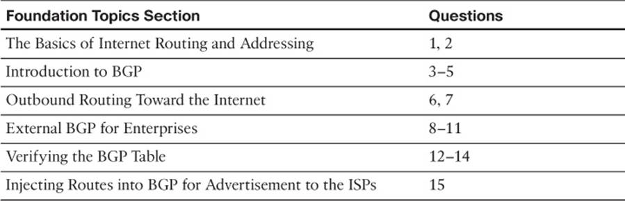
Table 13-1 “Do I Know This Already?” Foundation Topics Section-to-Question Mapping
1. Which of the following are considered private IPv4 addresses? (Choose two.)
a. 192.16.1.1
b. 172.30.1.1
c. 225.0.0.1
d. 127.0.0.1
e. 10.1.1.1
2. Class C network 200.1.1.0/24 was allocated to an ISP that operated primarily in Asia. That ISP then assigned this entire Class C network to one of its Asian customers. Network 200.1.2.0/24 has yet to be assigned to any ISP. Which of the following is most likely to be true?
a. 200.1.2.0/24 could be assigned to any registrar or ISP in the world.
b. 200.1.2.0/24 will be assigned in the same geography (Asia) as 200.1.1.0/24.
c. 200.1.2.0/24 cannot be assigned as public address space.
d. Routers inside North American ISPs increase their routing table size by 1 as a result of the customer with 200.1.1.0/24 connecting to the Internet.
3. Router R1, in ASN 11, learns a BGP route from BGP peer R22 in ASN 22. R1 and then uses BGP to advertise the route to R2, also in ASN 11. What ASNs would you see in the BGP table on R2 for this route?
a. 22
b. 11
c. 1
d. None
4. Which of the following are most likely to be used as an ASN by a company that has a registered public 16-bit ASN? (Choose two.)
a. 1
b. 65,000
c. 64,000
d. 64,550
5. Which of the following statements is true about a router’s eBGP peers that is not also true about that same router’s iBGP peers?
a. The eBGP peer neighborship uses TCP.
b. The eBGP peer uses port 180 (default).
c. The eBGP peer uses the same ASN as the local router.
d. The eBGP peer updates its AS_PATH PA before sending updates to this router.
6. Which of the following is the primary motivation for using BGP between an enterprise and its ISPs?
a. To influence the choice of best path (best route) for at least some routes
b. To avoid having to configure static routes
c. To allow redistribution of BGP routes into the IGP routing protocol
d. To monitor the size of the Internet BGP table
7. The following terms describe various design options for enterprise connectivity to the Internet. Which of the following imply that the enterprise connects to two or more ISPs? (Choose two.)
a. Single-homed
b. Dual-homed
c. Single-multihomed
d. Dual-multihomed
8. Enterprise Router R1, in ASN 1, connects to ISP Router I1, ASN 2, using eBGP. The single serial link between the two routers uses IP addresses 10.1.1.1 and 10.1.1.2, respectively. Both routers use their S0/0 interfaces for this link. Which of the following commands would be needed on R1 to configure eBGP? (Choose two.)
a. router bgp 2
b. router bgp 1
c. neighbor 10.1.1.2 remote-as 2
d. neighbor 10.1.1.2 update-source 10.1.1.1
e. neighbor 10.1.1.2 update-source S0/0
9. Enterprise Router R1, in ASN 1, connects to ISP Router I1, ASN 2, using eBGP. There are two parallel serial links between the two routers. The implementation plan calls for each router to base its BGP TCP connection on its respective loopback1 interfaces, with IP addresses 1.1.1.1 and 2.2.2.2, respectively. Which of the following commands would not be part of a working eBGP configuration on Router R1?
a. router bgp 1
b. neighbor 2.2.2.2 remote-as 2
c. neighbor 2.2.2.2 update-source loopback1
d. neighbor 2.2.2.2 multihop 2
10. The following output, taken from a show ip bgp summary command on Router R1, lists two neighbors. In what BGP neighbor state is neighbor 1.1.1.1?
...
Neighbor V AS MsgRcvd MsgSent TblVer InQ OutQ Up/Down State/PfxRcd
1.1.1.1 4 1 60 61 26 0 0 00:45:01 0
2.2.2.2 4 3 153 159 26 0 0 00:38:13 1
a. Idle
b. Opensent
c. Active
d. Established
11. The following output was taken from the show ip bgp summary command on Router R2. In this case, which of the following commands are most likely to already be configured on R2? (Choose two.)
...
BGP router identifier 11.11.11.11, local AS number 11
Neighbor V AS MsgRcvd MsgSent TblVer InQ OutQ Up/Down State/PfxRcd
1.1.1.1 4 1 87 87 0 0 0 00:00:06 Idle (Admin)
2.2.2.2 4 3 173 183 41 0 0 00:58:47 2
a. router bgp 11
b. neighbor 1.1.1.1 remote-as 11
c. neighbor 2.2.2.2 prefix-limit 1
d. neighbor 1.1.1.1 shutdown
12. Which of the following answers is most true about the BGP Update message?
a. It lists a set of path attributes, along with a list of prefixes that use those PAs.
b. It lists a prefix/length, plus the PA settings for that prefix.
c. It lists withdrawn routes, but never in the same Update message as newly advertised routes.
d. A single Update message lists at most a single prefix/length.
13. The following output occurs on Router R1. Which of the following cannot be determined from this output?
R1# show ip route 180.1.1.0 255.255.255.240
Routing entry for 180.1.1.0/28
Known via "bgp 2", distance 20, metric 0
Tag 3, type external
Last update from 192.168.1.2 00:10:27 ago
Routing Descriptor Blocks:
* 192.168.1.2, from 192.168.1.2, 00:10:27 ago
Route metric is 0, traffic share count is 1
AS Hops 2
Route tag 3
a. The type of BGP peer (iBGP or eBGP) that advertised this route to R1
b. R1’s ASN
c. The next-hop router’s ASN
d. The AS_PATH length
14. The following line of output was extracted from the output of the show ip bgp command on Router R1. Which of the following can be determined from this output?
...
Network Next Hop Metric LocPrf Weight Path
* 130.1.1.0/28 1.1.1.1 0 1 2 3 4 i
a. The route is learned from an eBGP peer.
b. The route has no more than three ASNs in the AS_PATH.
c. The route is the best route for this prefix.
d. None of these facts can be positively determined by this output.
15. Router R1 has eBGP connections to I1 and I2, routers at the same ISP. The company that owns R1 can use public address range 130.1.16.0/20. The following output lists all the IP routes in R1’s routing table within this range. Which of the following answers would cause R1 to advertise the 130.1.16.0/20 prefix to its eBGP peers? (You should assume default settings for any parameters not mentioned in this question.)
R1# show ip route 130.1.16.0 255.255.240.0 longer-prefixes
...
O 130.1.16.0/24 [110/3] via 10.5.1.1, 00:14:36, FastEthernet0/1
O 130.1.17.0/24 [110/3] via 10.5.1.1, 00:14:36, FastEthernet0/1
O 130.1.18.0/24 [110/3] via 10.5.1.1, 00:14:36, FastEthernet0/1
a. Configure R1 with the network 130.1.16.0 mask 255.255.240.0 command.
b. Configure R1 with the network 130.1.16.0 mask 255.255.240.0 summary-only command.
c. Redistribute from OSPF into BGP, filtering so that only routes in the 130.1.16.0/20 range are redistributed.
d. Redistribute from OSPF into BGP, filtering so that only routes in the 130.1.16.0/20 range are redistributed, and create a BGP summary for 130.1.16.0/20.
Foundation Topics
The Basics of Internet Routing and Addressing
The original design for the Internet called for the assignment of globally unique IPv4 addresses for all hosts connected to the Internet. The idea is much like the global telephone network, with a unique phone number, worldwide, for all phone lines, cell phones, and so on.
To achieve this goal, the design called for all organizations to register and be assigned one or more public IP networks (Class A, B, or C). Then, inside that organization, each address would be assigned to a single host. By using only the addresses in their assigned network number, each company’s IP addresses would not overlap with other companies. As a result, all hosts in the world would have globally unique IP addresses.
The assignment of a single classful network to each organization actually helped keep Internet routers’ routing tables small. The Internet routers could ignore all subnets used inside each company, and instead just have a route for each classful network. For example, if a company registered and was assigned Class B network 128.107.0.0/16, and had 500 subnets, the Internet routers just needed one route for that entire Class B network.
Over time, the Internet grew tremendously. It became clear by the early 1990s that something had to be done, or the growth of the Internet would grind to a halt. At the then-current rate of assigning new networks, all public IP networks would soon be assigned and growth would be stifled. Additionally, even with routers ignoring the specific subnets, the routing tables in Internet routers were becoming too large for the router technology of that day. (For perspective, more than 2 million public Class C networks exist, and 2 million IP routes in a single IP routing table would be considered quite large—maybe even too large—for core routers in the Internet even today.)
To deal with these issues, the Internet community worked together to come up with both some short-term and long-term solutions to two problems: the shortage of public addresses and the size of the routing tables. The short-term solutions to these problems included
![]() Reduce the number of wasted public IP addresses by using classless IP addressing when assigning prefixes, assigning prefixes/lengths instead of being restricted to assigning only Class A, B, and C network numbers.
Reduce the number of wasted public IP addresses by using classless IP addressing when assigning prefixes, assigning prefixes/lengths instead of being restricted to assigning only Class A, B, and C network numbers.
![]() Reduce the need for public IP addresses by using Port Address Translation (PAT, also called NAT overload) to multiplex more than 65,000 concurrent flows using a single public IPv4 address.
Reduce the need for public IP addresses by using Port Address Translation (PAT, also called NAT overload) to multiplex more than 65,000 concurrent flows using a single public IPv4 address.
![]() Reduce the size of IP routing tables by making good choices for how address blocks are allocated to ISPs and end users, allowing for route summarization on a global scale.
Reduce the size of IP routing tables by making good choices for how address blocks are allocated to ISPs and end users, allowing for route summarization on a global scale.
This section examines some of the details related to these three points, but this information is not an end to itself for the purposes of this book. The true goal is to understand outbound routing (from the enterprise to the Internet), and the reasons why you might or might not need to use a dynamic routing protocol, such as Border Gateway Protocol (BGP), between the enterprise and the Internet.
Public IP Address Assignment
The Internet Corporation for Assigned Names and Numbers (ICANN, www.icann.org) owns the processes by which public IPv4 (and IPv6) addresses are allocated and assigned. A related organization, the Internet Assigned Numbers Authority (IANA, www.iana.org) carries out many of ICANN’s policies. These organizations define which IPv4 addresses can be allocated to different geographic regions, in addition to managing the development of the Domain Name System (DNS) naming structure and new Top Level Domains (TLD), such as domains ending in .com.
ICANN works with several other groups to administer a public IPv4 address assignment strategy that can be roughly summarized as follows:
Step 1. ICANN and IANA group public IPv4 addresses by major geographic region.
Step 2. IANA allocates those address ranges to Regional Internet Registries (RIR).
Step 3. Each RIR further subdivides the address space by allocating public address ranges to National Internet Registries (NIR) or Local Internet Registries (LIR). (ISPs are typically LIRs.)
Step 4. Each type of Internet Registry (IR) can assign a further subdivided range of addresses to the end-user organization to use.
Figure 13-1 shows an example that follows the same preceding four-step sequence. In this example, a company in North America needs a subnet with six hosts, so the ISP assigns a /29 prefix (198.133.219.16/29). Before that happens, however, the process gave this company’s ISP (NA-ISP1, an ISP in North America) the right to assign that particular prefix.

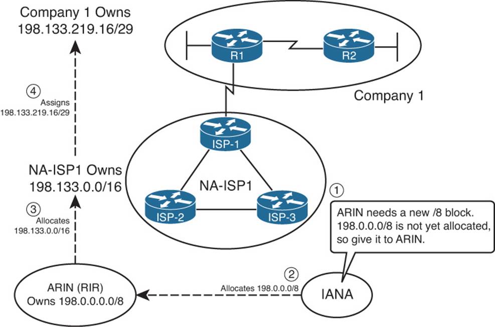
Figure 13-1 Conceptual View of Public IPv4 Address Assignment
The process starts with ICANN and IANA. These organizations maintain a set of currently unallocated public IPv4 addresses. (See www.iana.org/numbers, and look for the IPv4 addresses link to see the current list.) When the American Registry for Internet Numbers (ARIN), the RIR for North America, notices that it is running out of IPv4 address space, ARIN requests a new public address block. IANA examines the request, finds a currently unallocated public address block (Step 1 in the figure), and allocates the block to ARIN (Step 2 in the figure).
Next, an ISP named NA-ISP1 (shorthand for North American ISP number 1) asks ARIN for a prefix assignment for a /16-sized address block. After ARIN ensures that NA-ISP1 meets some requirements, ARIN assigns a prefix of 198.133.0.0/16 (Step 3 in the figure). Then, when Company1 becomes a customer of NA-ISP1, NA-ISP1 can assign a prefix to Company 1 (198.133.219.16/29 in this example, Step 4).
Although the figure shows the process, the big savings for public addresses occur because the user of the IP addresses can be assigned a group much smaller than a single Class C network. In some cases, companies only need one public IP address; in other cases, they might need only a few, as with Company1 in Figure 13-1. This practice allows IRs to assign the right-sized address block to each customer, reducing waste.
Note
On January 31, 2011, ICANN gave out its last two blocks of IPv4 addresses meant for general usage. This left only five blocks of usable addresses. ICANN’s “Global Policy for the Allocation of the Remaining IPv4 Address Space” policy dictates how those remaining blocks (one for each Regional Internet Registry) will be given out as we approach the exhaustion of IPv4 addresses.
Internet Route Aggregation
Although the capability to assign small blocks of addresses helped extend the IPv4 public address space, this practice also introduced many more public subnets into the Internet, driving up the number of routes in Internet routing tables. At the same time, the number of hosts connected to the Internet, back in the 1990s, was increasing at a double-digit rate per month. Internet core routers could not have kept up with the rate of increase in the size of the IP routing tables.
The solution was, and still is today, to allocate numerically consecutive addresses—addresses that can be combined into a single route prefix/length—by geography and by ISP. These allocations significantly aid route summarization.
For example, continuing the same example shown in Figure 13-1, Figure 13-2 shows some of the routes that can be used in ISPs around the globe based on the address assignment shown in Figure 13-1.
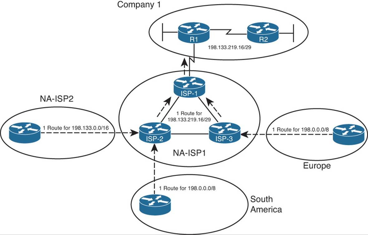
Figure 13-2 IPv4 Global Route Aggregation Concepts
First, focus on the routers shown in Europe and South America. Routers outside North America can use a route for prefix 198.0.0.0/8, knowing that IANA assigned this prefix to be used only by ARIN, which manages IP addresses in North America. The underlying logic is that if the routers outside North America can forward a packet into North America, the North American routers will have more specific routes. The single route for 198.0.0.0/8 shown in Europe and South America can be used instead of literally millions of subnets deployed to companies in North America, such as Company1.
Next, consider routers in North America, specifically those outside the NA-ISP1 network. Figure 13-2 shows one such ISP, named NA-ISP2 (North American ISP number 2), on the left. This router can learn one route for 198.133.0.0/16, the portion of the 198.0.0.0/8 block assigned to NA-ISP1 by IANA. Routers in NA-ISP2 can forward all packets for destinations inside this prefix to NA-ISP1, rather than needing a route for all small address blocks assigned to individual enterprises such as Company1. This significantly reduces the number of routes required on NA-ISP2 routers.
Finally, inside NA-ISP1, its routers need to know to which NA-ISP1 router to forward packets for that particular customer. So, the routes listed on NA-ISP1’s routers lists a prefix of 198.133.219.16/29. As a result, packets are forwarded toward Router ISP-1 (located inside ISP NA-ISP1), and finally into Company 1.
The result of the summarization inside the Internet allows Internet core routers to have a much smaller routing table—on the order of a few hundred thousand routes instead of a few tens of millions of routes. For perspective, the website www.potaroo.net, a website maintained by Geoff Huston, who has tracked Internet growth for many years, lists a statistic showing approximately 480,000 BGP routes in Internet routers back in February 2014.
The Impact of NAT/PAT
Although classless public IP address assignment does help extend the life of the IPv4 address space, NAT probably has a bigger positive impact, because it enables an enterprise to use such a small number of public addresses. NAT allows an enterprise to use private IP addresses for each host, plus a small number of public addresses. As packets pass through a device performing NAT—often a firewall, but it could be a router—the NAT function translates the IP address from the private address (called an inside local address by NAT) into a public address (called an inside global address).
Note
For the purposes of this book, the terms NAT, PAT, and NAT overload are used synonymously. There is no need to distinguish between static NAT, dynamic NAT without overload, and dynamic NAT with overload (also called PAT).
NAT reduces the need for public IPv4 addresses to only a few addresses per enterprise because of how NAT can multiplex flows using different TCP or UDP port numbers. Figure 13-3 shows a sample that focuses on a router performing NAT. The figure shows an enterprise network on the left, with the enterprise using private Class A network 10.0.0.0/8. The Internet sits on the right, with the NAT router using public IP address 200.1.1.2.
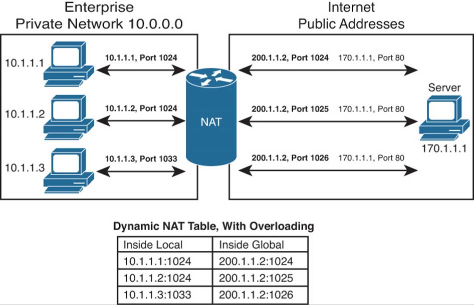
Figure 13-3 IPv4 Global Route Aggregation Concepts
The figure shows how the enterprise, on the left, can support three flows with a single public IP address (200.1.1.2). The NAT feature dynamically builds its translation table, which tells the router what address/port number pairs to translate. The router reacts when a new flow occurs between two hosts, noting the source IP address and port number of the enterprise host on the left, and translating those values to use the public IP address (200.1.1.2) and an unused port number in the Internet. Note that if you collected the traffic using a network analyzer on the right side of the NAT router, the IP addresses would include 200.1.1.2 but not any of the network 10.0.0.0/8 addresses. Because the combination of the IP address (200.1.1.2 in this case) and port number must be unique, this one IP address can support 216 different concurrent flows.
Private IPv4 Addresses and Other Special Addresses
When allocating the public IPv4 address space, IANA/ICANN restricts themselves in several ways. Of course, the private IP address ranges cannot be assigned to any group for use in the public Internet. Additionally, several other number ranges inside the IPv4 address space, as summarized in RFC 3330, are reserved for various reasons. Tables 13-2 and 13-3 list the private addresses and other reserved values, respectively, for your reference.
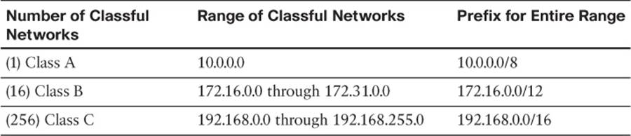
Table 13-2 Private IP Address Reference
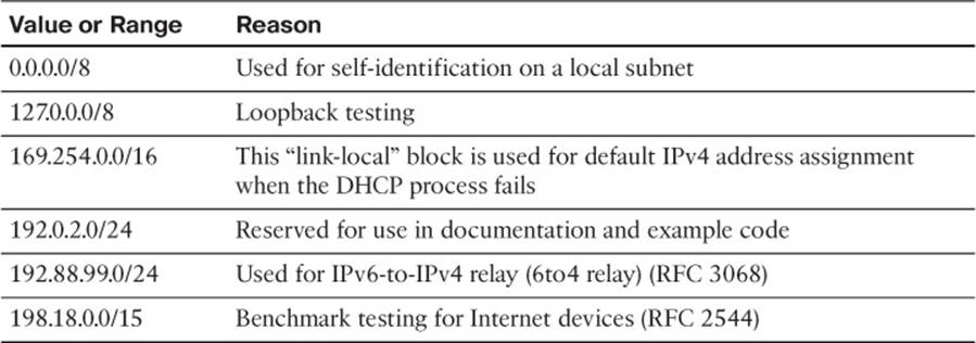
Table 13-3 Reserved Values in IPv4 Address Range (RFC 3330)
Table 13-3 lists other reserved ranges of IPv4 addresses that IANA will not allocate in the public Internet.
In summary, every enterprise that connects to the Internet must use at least one public IP address and often several public IP addresses. Although some companies do have a large public IPv4 address block—often obtained before the shortage of public IPv4 addresses in the early to mid-1990s—most companies have a small address block, which then requires the use of NAT/PAT. These details have some impact on whether BGP is useful in a given case.
Introduction to BGP
Border Gateway Protocol (BGP) advertises, learns, and chooses the best paths inside the global Internet. When two ISPs connect, they typically use BGP to exchange routing information. Collectively, the ISPs of the world exchange the Internet’s routing table using BGP. And enterprises sometimes use BGP to exchange routing information with one or more ISPs, allowing the enterprise routers to learn Internet routes.
One key difference when comparing BGP to the usual IGP routing protocols is BGP’s robust best-path algorithm. BGP uses this algorithm to choose the best BGP path (route) using rules that extend far beyond just choosing the route with the lowest metric. This more complex best-path algorithm gives BGP the power to let engineers configure many different settings that influence BGP best-path selection, allowing great flexibility in how routers choose the best BGP routes.
BGP Basics
BGP, specifically BGP version 4 (BGPv4), is the one routing protocol in popular use today that was designed as an exterior gateway protocol (EGP) instead of as an interior gateway protocol (IGP). As such, some of the goals of BGP differ from those of an IGP, such as Open Shortest Path First (OSPF) or Enhanced Interior Gateway Routing Protocol (EIGRP), but some of the goals remain the same.
First, consider the similarities between BGP and various IGPs. BGP does need to advertise IPv4 prefixes, just like IGPs. BGP needs to advertise some information, so that routers can choose one of many routes for a given prefix as the currently best route. As for the mechanics of the protocol, BGP does establish a neighbor relationship before exchanging topology information with a neighboring router.
Next, consider the differences. BGP does not require neighbors to be attached to the same subnet. Instead, BGP routers use a TCP connection (port 179) between the routers to pass BGP messages, allowing neighboring routers to be on the same subnet or to be separated by several routers. (It is relatively common to see BGP neighbors who do not connect to the same subnet.) Another difference lies in how the routing protocols choose the best route. Instead of choosing the best route just by using an integer metric, BGP uses a more complex process, using a variety of information, called BGP path attributes (PAs), which are exchanged in BGP routing updates much like IGP metric information.
Table 13-4 summarizes some of these key comparison points.
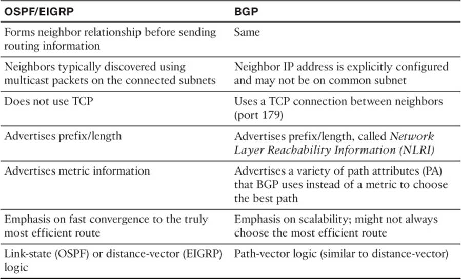
Table 13-4 Comparing OSPF and EIGRP Logic to BGP
Note
BGP also uses the term Network Layer Reachability Information (NLRI) to describe the IP prefix and length. This book uses the more familiar term prefix.
BGP ASNs and the AS_SEQ Path Attribute
BGP uses BGP path attributes for several purposes. PAs define information about a path, or route, through a network. Some BGP PAs describe information that can be useful in choosing the best BGP route, using the best-path algorithm. BGP also uses some PAs for purposes other than choosing the best path.
By default, if no BGP PAs have been explicitly set, BGP routers use the BGP AS_PATH (autonomous system path) PA when choosing the best route among many competing routes. The AS_PATH PA itself has many subcomponents, only some of which matter to the depth of the CCNP coverage of the topic. However, the most obvious component of AS_PATH, the AS_SEQ (AS_SEQUENCE), can be easily explained with an example when the concept of an autonomous system number (ASN) has been explained.
The integer BGP ASN uniquely identifies one organization that considers itself autonomous from other organizations. Each company whose enterprise network connects to the Internet can be considered to be an autonomous system and can be assigned a BGP ASN. (IANA/ICANN also assigns globally unique ASNs.) Additionally, each ISP has an ASN, or possibly several, depending on the size of the ISP.
When a router uses BGP to advertise a route, the prefix/length is associated with a set of PAs, including the AS_PATH. The AS_PATH PA associated with a prefix/length lists the ASNs that would be part of an end-to-end route for that prefix as learned using BGP. In a way, the AS_PATH implies information like this: “If you use this path (route), the path will go through this list of ASNs.”
BGP uses the AS_PATH to perform two key functions:
![]() Choose the best route for a prefix based on the shortest AS_PATH (fewest number of ASNs listed).
Choose the best route for a prefix based on the shortest AS_PATH (fewest number of ASNs listed).
![]() Prevent routing loops.
Prevent routing loops.
An example can help demonstrate the concept. This example, and some others in this chapter, uses the design shown in Figure 13-4. This network has five ASNs: three ISPs and two customers.
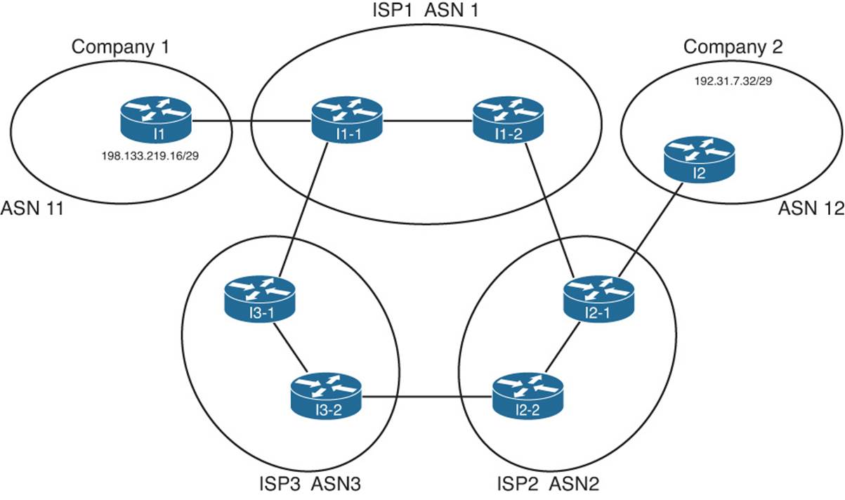
Figure 13-4 Sample Portion of the Internet
Figure 13-4 shows only a couple of routers in each ISP, and it also does not bother to show much of the enterprise networks for the two companies. However, the diagram does show enough detail to demonstrate some key BGP concepts. For the sake of discussion, assume that each line between routers represents some physical medium that is working. Each router will use BGP, and each router will form BGP neighbor relationships with the routers on the other end of each link. For example, ISP1’s I1-2 router will have a BGP neighbor relationship with Routers I1-1 and I2-1.
With that in mind, consider Figure 13-5, which shows the advertisement of BGP updates for prefix 192.31.7.32/29 to the other ASNs. The figure shows four steps, as follows:
Step 1. I2, in ASN 12, advertises the route outside ASN 12. So, I2 adds its own ASN (12) to the AS_PATH PA when advertising the route.
Step 2. The routers inside ASN 2, when advertising the route outside ASN 2, add their own ASN (2) to the AS_PATH PA when advertising the route. Their advertised AS_PATH is then (12,2).
Step 3. Router I3-1, inside ASN 3, had previously learned about the route for 192.31.7.32/29 from ASN 2, with AS_PATH (12,2). So, I3-1 advertises the route to ASN 1, after adding its own ASN (3) to the AS_PATH so that the AS_PATH is (12,2,3).
Step 4. Similarly, Router I1-1, inside ASN 1, advertises the route to ASN3. Because ASN 3 is a different ASN, I1-1 adds its own ASN (1) to the AS_PATH PA so that the AS_PATH lists ASNs 12, 2, and 1.
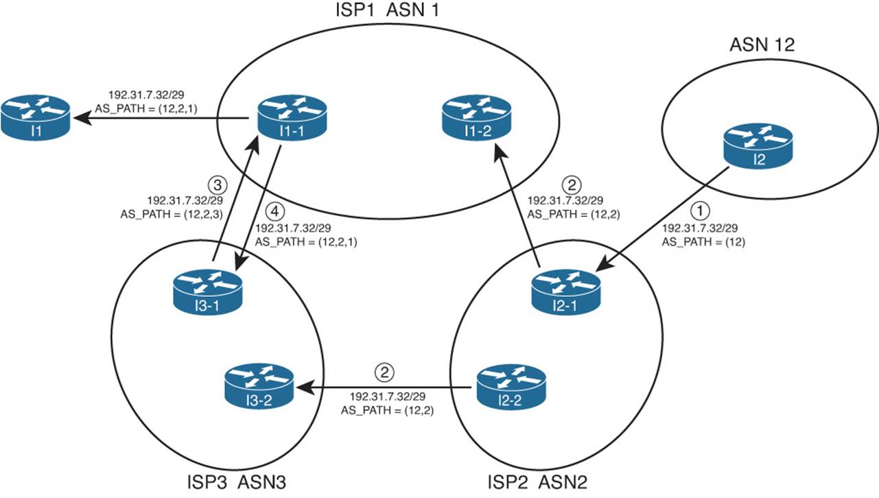
Figure 13-5 Advertisement of NLRI to Demonstrate AS_PATH
Now, step back from the details, and consider the two alternative routes learned collectively by the routers in ASN 1:
![]() 192.31.7.32/29, AS_PATH (12,2)
192.31.7.32/29, AS_PATH (12,2)
![]() 192.31.7.32/29, AS_PATH (12,2,3)
192.31.7.32/29, AS_PATH (12,2,3)
Because the BGP path selection algorithm uses the shortest AS_PATH, assuming that no other PAs have been manipulated, the routers in ASN 1 use the first of the two paths, sending packets to ASN 2 next, and not using the path through ASN 3. Also, as a result, note that the advertisement from ASN 1 into ASN 11 lists an AS_PATH that reflects the best-path selection of the routers inside ASN 1, with the addition of ASN 1 to the end of the AS_PATH of the best route (12,2,1).
BGP routers also prevent routing loops using the ASNs listed in the AS_PATH. When a BGP router receives an update, and a route advertisement lists an AS_PATH with its own ASN, the router ignores that route. This is because the route has already been advertised through the local ASN; to believe the route and then advertise it further might cause routing loops.
Internal and External BGP
BGP defines two classes of neighbors (peers): internal BGP (iBGP) and external BGP (eBGP). These terms use the perspective of a single router, with the terms referring to whether a BGP neighbor is in the same ASN (iBGP) or a different ASN (eBGP).
A BGP router behaves differently in several ways depending on whether the peer (neighbor) is an iBGP or eBGP peer. The differences include different rules about what must be true before the two routers can become neighbors, different rules about which routes the BGP best-path algorithm chooses as best, and even some different rules about how the routers update the BGP AS_PATH PA.
When advertising to an eBGP peer, a BGP router updates the AS_PATH PA, but it does not do so when advertising to an iBGP peer. For example, Figure 13-6 shows the same design, with the same route advertisement, as in Figure 13-5. However, in this case, all the BGP connections have been listed as either iBGP or eBGP.
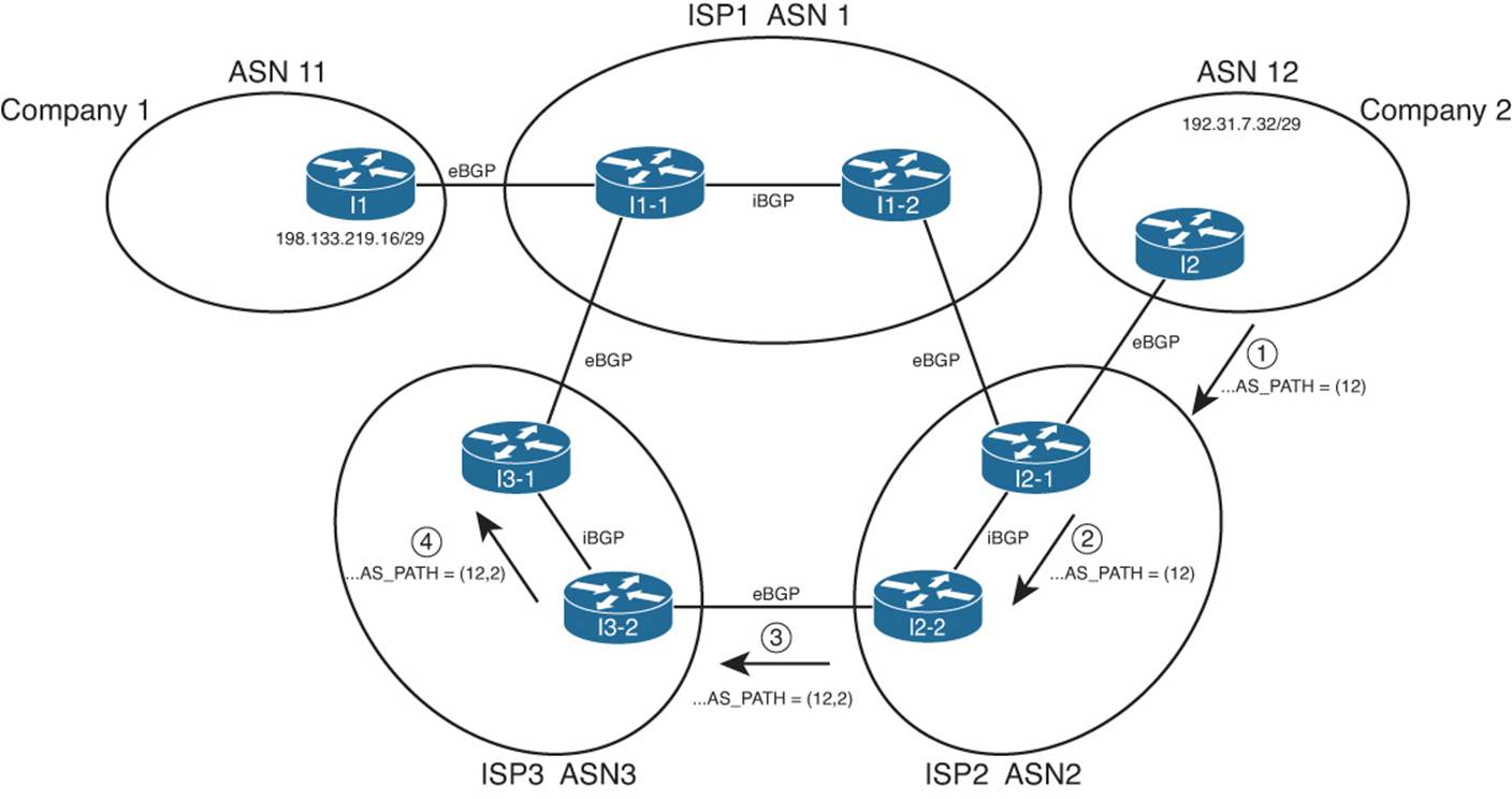
Figure 13-6 iBGP, eBGP, and Updating AS_PATH for eBGP Peers
The figure highlights the route advertisement from ASN 12, over the lower path through ASN 2 and 3. Note that at Step 1, Router I2, advertising to an eBGP peer, adds its own ASN to the AS_PATH. At Step 2, Router I2-1 is advertising to an iBGP peer (I2-2), so it does not add its own ASN (2) to the AS_PATH. Then, at Step 3, Router I2-2 adds its own ASN (2) to the AS_PATH before sending an update to eBGP peer I3-2, and so on.
Public and Private ASNs
For the Internet to work well using BGP, IANA administers the assignment of ASNs much like it does with IP address prefixes. One key reason why ASNs must be assigned as unique values is that if ASNs are duplicated, the BGP loop-prevention process can actually prevent parts of the Internet from learning about a route. For example, consider Figure 13-7, with the same design as in the last few figures—but this time with a duplicate ASN.
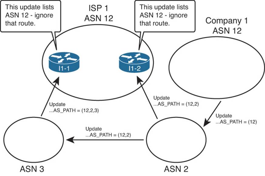
Figure 13-7 Duplicate ASN (12) Preventing Route Advertisement
In this figure, both ISP1 and Company 1 use ASN 12. The example’s BGP updates begin as in Figures 13-5 and 13-6, with Company 1 advertising its prefix. Routers inside ISP1 receive BGP updates that list the same prefix used by Company 1, but both Updates list an AS_PATH that includes ASN 12. Because ISP1 thinks it uses ASN 12, ISP1 thinks that these BGP Updates should be ignored as part of the BGP loop-prevention process. As a result, customers of ISP1 cannot reach the prefixes advertised by routers in Company 1.
To prevent such issues, IANA controls the ASN numbering space. Using the same general process as for IPv4 addresses, ASNs can be assigned to different organizations. The 16-bit BGP ASN implies a decimal range of 0 through 65,535. Table 13-5 shows some of the details of IANA’s current ASN assignment conventions.
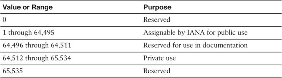
Table 13-5 16-Bit ASN Assignment Categories from IANA
Like the public IPv4 address space has suffered with the potential for complete depletion of available addresses, the public BGP ASN space has similar issues. To help overcome this issue, the ASN assignment process requires that each AS justify whether it truly needs a publicly unique ASN or whether it can just as easily use a private ASN. Additionally, RFC 5398 reserves a small range of ASNs for use in documentation, so that the documents can avoid the use of ASNs assigned to specific organizations.
Private ASNs allow the routers inside an AS to participate with BGP, while using the same ASN as many other organizations. Most often, an AS can use a private AS in cases where the AS connects to only one other ASN. (Private ASNs can be used in some cases of connecting to multiple ASNs as well.) The reason is that with only one connection point to another ASN, loops cannot occur at that point in the BGP topology, so the need for unique ASNs in that part of the network no longer exists. (The loops cannot occur because of the logic behind the BGP best-path algorithm, coupled with the fact that BGP only advertises the best path for a given prefix.)
Outbound Routing Toward the Internet
The single biggest reason to consider using BGP between an enterprise and an ISP is to influence the choice of best path (best route). The idea of choosing the best path sounds appealing at first. However, because the majority of the end-to-end route exists inside the Internet, particularly if the destination is 12 routers and a continent away, it can be a challenge to determine which exit point from the enterprise is actually a better route.
As a result, enterprises typically have two major classes of options for outbound routing toward the Internet: default routing and BGP. Using default routes is perfectly reasonable, depending on the objectives. This section examines the use of default routes toward the Internet, and describes some of the typical enterprise BGP designs and how they can be used to influence outbound routes toward the Internet.
Comparing BGP and Default Routing for Enterprises
A default static route is a statically configured route that can be used by a router if a more specific route to a destination network is not found in the router’s IP routing table. Oftentimes, a branch office router uses a default static route pointing toward the core of a network. The WAN edge routers then needed static routes for the subnets at each branch, with the WAN edge routers advertising these branch subnets into the core using an IGP.
The branch office default routing design results in less processing on the routers, less memory consumption, and no IGP overhead on the link between the branch and WAN distribution routers. Specifically, the branch routers can have a single or a few default routes, instead of potentially hundreds of routes for specific prefixes, all with the same next-hop information.
The same general concept of using defaults and static routes at enterprise branches can be applied to the enterprise network and its connections to one or a few ISPs. Similar to a branch router, an entire enterprise often has only a few connections to the Internet. If one of those connections is considered better than the others, all packets sent from the enterprise toward the Internet would normally follow that one Internet link, for all Internet destinations. Likewise, the ISPs, similar to WAN distribution routers in this analogy, could configure static routes for the enterprise’s public IP address prefix and then use BGP in the Internet to advertise those routes. Figure 13-8 illustrates this idea.
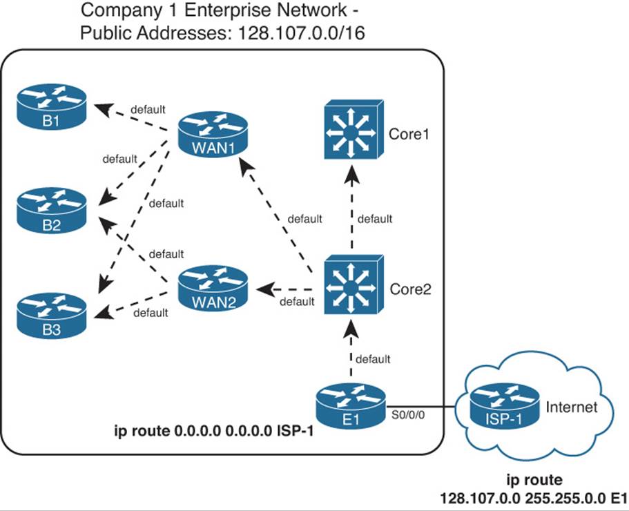
Figure 13-8 Use of Static Default into the Internet
Although the enterprise could choose to use BGP in this case, such a decision is not automatic. First, the alternative of using static routes, as shown in the figure, does not require a lot of work. The enterprise network engineer just needs to configure a default route and advertise it throughout the enterprise; the dashed lines in the figure represent the advertisement of the default route with the enterprise’s IGP.
In addition to the configuration on the enterprise router (E1), the ISP network engineer has to configure static routes for that enterprise’s public IP address range, and redistribute those routes into BGP to advertise them throughout the Internet. The figure shows a static route for Company 1’s 128.107.0.0/16 public address range. Additionally, this prefix would need to be injected into BGP for advertising into the rest of the Internet.
Instead of using static default routes, you could enable BGP between E1 and ISP-1. Running BGP could mean that the enterprise router requires significant memory and more processing power on the router. The design might also require other enterprise routers besides the Internet-connected routers to know the BGP routes, requiring additional routers to have significant CPU and memory resources. Finally, although you can configure BGP to choose one route over another using PAs, the advantage of choosing one path over another might not be significant. Alternatively, you could ask the ISP to advertise only a default route with BGP.
Now that you have seen a few of the reasons why you might be fine using static routes instead of BGP, consider why you might want to use BGP. First, it makes the most sense to use BGP when you have at least two Internet connections. Second, BGP becomes most useful when you want to choose one outbound path over another path for particular destinations in the Internet. In short, when you have multiple Internet connections, and you want to influence some packets to take one path and some packets to take another, consider BGP.
This chapter next examines different cases of Internet connectivity and weighs the reasons why you might choose to use BGP. For this discussion, the perspective of the enterprise network engineer will be used. As such, outbound routing is considered to be routing that direct packets from the enterprise network toward the Internet, and inbound routing refers to routing that direct packets into the enterprise network from the Internet.
To aid in the discussion, this section examines four separate cases:
![]() Single-homed (1 link per ISP, 1 ISP)
Single-homed (1 link per ISP, 1 ISP)
![]() Dual-homed (2+ links per ISP, 1 ISP)
Dual-homed (2+ links per ISP, 1 ISP)
![]() Single-multihomed (1 link per ISP, 2+ ISPs)
Single-multihomed (1 link per ISP, 2+ ISPs)
![]() Dual-multihomed (2+ links per ISP, 2+ ISPs)
Dual-multihomed (2+ links per ISP, 2+ ISPs)
Note
The terms in the preceding list can be used differently depending on what book or document you read. For consistency, this book uses these terms in the same way as the Cisco authorized ROUTE course associated with the ROUTE exam.
Single-Homed
The single-homed Internet design uses a single ISP, with a single link between the enterprise and the ISP. With single-homed designs, only one possible next-hop router exists for any and all routes for destinations in the Internet. As a result, no matter what you do with BGP, all learned routes would list the same outgoing interface for every route, which minimizes the benefits of using BGP.
Single-homed designs often use one of two options for routing to and from the Internet:
![]() Use static routes (default in the enterprise, and a static route for the enterprise’s public address range at the ISP).
Use static routes (default in the enterprise, and a static route for the enterprise’s public address range at the ISP).
![]() Use BGP, but only to exchange a default route (ISP to enterprise) and a route for the enterprise’s public prefix (enterprise to ISP).
Use BGP, but only to exchange a default route (ISP to enterprise) and a route for the enterprise’s public prefix (enterprise to ISP).
The previous section already showed the main concepts for the first option. For the second option, the concept still uses the IGP’s mechanisms to flood a default route throughout the enterprise, causing all packets to go toward the Internet-facing router. Instead of using static routes, however, the following must happen:
![]() The ISP router uses BGP to advertise a default route to the enterprise.
The ISP router uses BGP to advertise a default route to the enterprise.
![]() You must configure the IGP on the enterprise’s Internet-facing router to flood a default route (typically only if the default route exists in that router’s routing table).
You must configure the IGP on the enterprise’s Internet-facing router to flood a default route (typically only if the default route exists in that router’s routing table).
![]() You must configure BGP on the enterprise router and advertise the enterprise’s public prefix toward the ISP.
You must configure BGP on the enterprise router and advertise the enterprise’s public prefix toward the ISP.
Both options—using static default routes and BGP-learned default routes—have some negatives. Some packets for truly nonexistent destinations flow through the enterprise to the Internet-facing router (E1 in the example of Figure 13-8) and over the link to the Internet, before being discarded for lack of a matching route. For example, if the enterprise used private network 10.0.0.0/8 internally, packets destined for addresses in network 10.0.0.0/8 that have not yet been deployed will match the default route and be routed to the Internet.
To avoid wasting this bandwidth by sending packets unnecessarily, a static route for 10.0.0.0/8, destination null0, could be added to the Internet-facing router but not advertised into the rest of the enterprise. (This type of route is sometimes called a discard route.) This route would prevent the Internet-facing router from forwarding packets destined for network 10.0.0.0/8 into the Internet.
Dual-Homed
The dual-homed design has two (or more) links to the Internet, but with all links connecting to a single ISP. This type of design can use a pair of routers, two pairs, or a combination, as shown in the three cases in Figure 13-9.
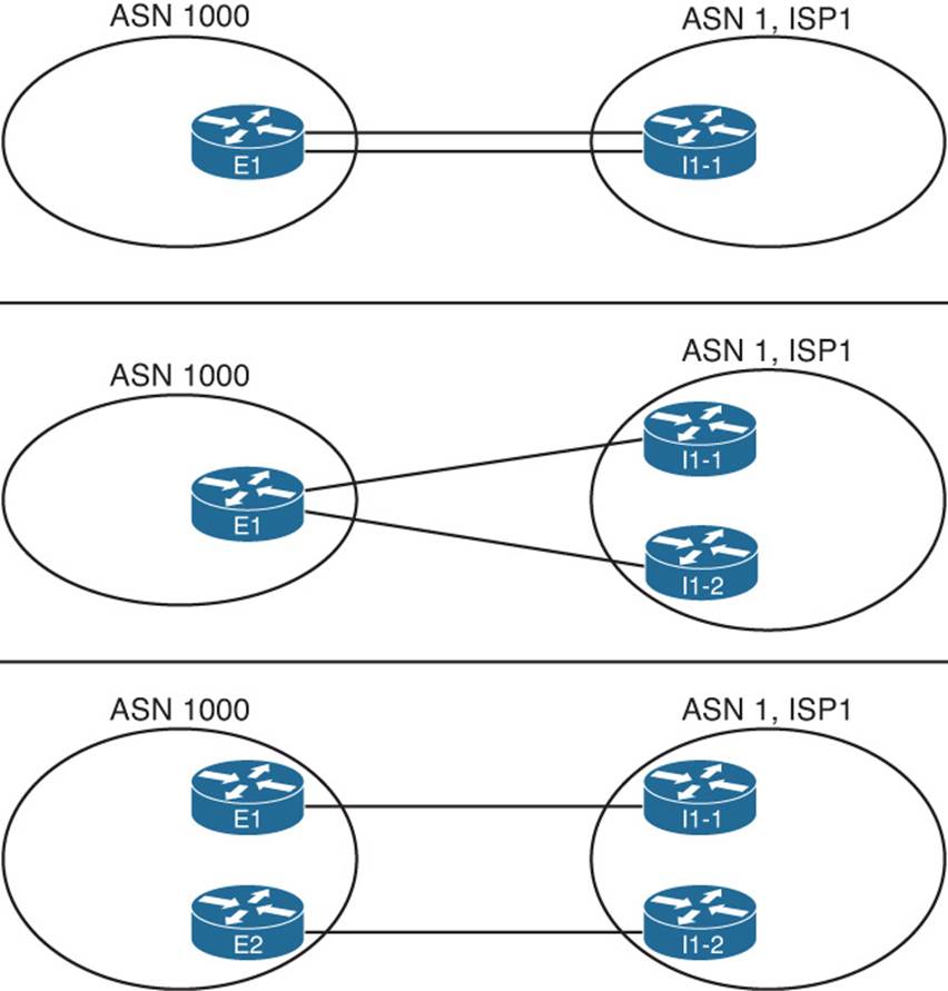
Figure 13-9 Dual-Homed Design Options
Comparing the dual-homed case to the single-homed design, the second link gives the enterprise a choice. The enterprise router(s) could choose between one of two links, and in the case with two enterprise routers, the choice of a different link also means the choice of sending packets to a different router.
Each of the cases shown in Figure 13-9 is interesting, but the case with two enterprise routers provides the most ideas to consider. When considering whether to use BGP in this case, and if so, how to use it, first think about whether you want to influence the choice of outbound route. The common cases when using defaults works well, ignoring BGP, are
![]() To prefer one Internet connection over another for all destinations, but when the better ISP connection fails, all traffic reroutes over the secondary connection.
To prefer one Internet connection over another for all destinations, but when the better ISP connection fails, all traffic reroutes over the secondary connection.
![]() To treat both Internet connections as equal, sending packets for some destinations out each path. However, when one fails, all traffic reroutes over the one still-working path.
To treat both Internet connections as equal, sending packets for some destinations out each path. However, when one fails, all traffic reroutes over the one still-working path.
The text now examines each option, in order, including a discussion of how to choose the best outbound routing using both partial and full BGP updates.
Preferring One Path over Another for All Destinations
When the design calls for one of the two Internet connections to always be preferred, regardless of destination, BGP can be used, but it is not required. With a goal of preferring one path over another, the routers can use default routes into the Internet.
To demonstrate the concept, Figure 13-10 shows a dual-homed design, this time with two routers (E1 and E2) connected to the Internet. Each router has a single link into the single ISP. Figure 13-10 shows the routes that result from using default routes to forward all traffic toward Router E1.
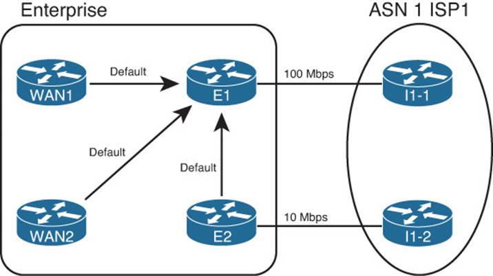
Figure 13-10 Dual-Homed Design, Using Defaults to Favor One Link
Figure 13-10 shows that all routers forward the Internet-destined packets toward Router E1, because this router has the faster Internet connection to ISP1 (100 Mbps in this case). Again in this example, the other connection from Router E2 to ISP1 uses a 10-Mbps link.
To make this design work, with failover, both E1 and E2 need to advertise a default route into the enterprise, but the route advertised by the primary router (E1) needs to have metrics set so that it is always the better of the two routes. For example, with EIGRP, E1 can configure a static default route with Router I1-1 as the next hop, but with very high bandwidth and very low delay upon redistribution into EIGRP. Conversely, E2 can create a default for Router I1-2 as the next-hop router, but with a low bandwidth but high delay. Example 13-1 shows the configuration of the static default route on both E1 and E2, with the redistribute command setting the metrics.
Note
With EIGRP as the IGP, remember that the delay setting must be set higher to avoid cases where some routers forward packets toward the secondary Internet router (E2). The reason is that EIGRP uses constraining bandwidth, so a high setting of bandwidth at the redistribution point on E1 might or might not cause more remote routers to use that route.
Example 13-1 Default Routing on Router E1
! Configuration on router E1 – note that the configuration uses
! a hostname instead of I1-1's IP address
ip route 0.0.0.0 0.0.0.0 I1-1
router eigrp 1
redistribute static metric 100000 1 255 1 1500
! Configuration on router E2 - note that the configuration uses
! a hostname instead of I1-2's IP address
ip route 0.0.0.0 0.0.0.0 I1-2
router eigrp 1
redistribute static metric 10000 100000 255 1 1500
A slightly different approach can be taken in other variations of the dual-homed design, as seen back in Figure 13-9. The first two example topologies in that figure show a single router with two links to the same ISP. If the design called for using one link as the preferred link, and the engineer decided to use default routes, that one router would need two default routes. To make one route be preferred, that static default route would be assigned a better administrative distance (AD) than the other route. For example, the commands ip route 0.0.0.0 0.0.0.0 I1-1 3 and ip route 0.0.0.0 0.0.0.0 I1-2 4 could be used on Router E1 in Figure 13-9, giving the route through I1-1 a lower AD (3), preferring that route. If the link to I1-1 failed, the other static default route, through I1-2, would be used.
Choosing One Path over Another Using BGP
The big motivation to use BGP occurs when you want to influence which link is used for certain destinations in the Internet. To see such a case, consider Figure 13-11, which adds Company 3 to the design. In this case, Company 3 uses prefix 192.135.250.0/28 as its public address range. Company 3 might be located closer to I1-2 inside ISP1 than to Router I1-1, and in such cases, the BGP design calls for making the packets flow over the route as shown.
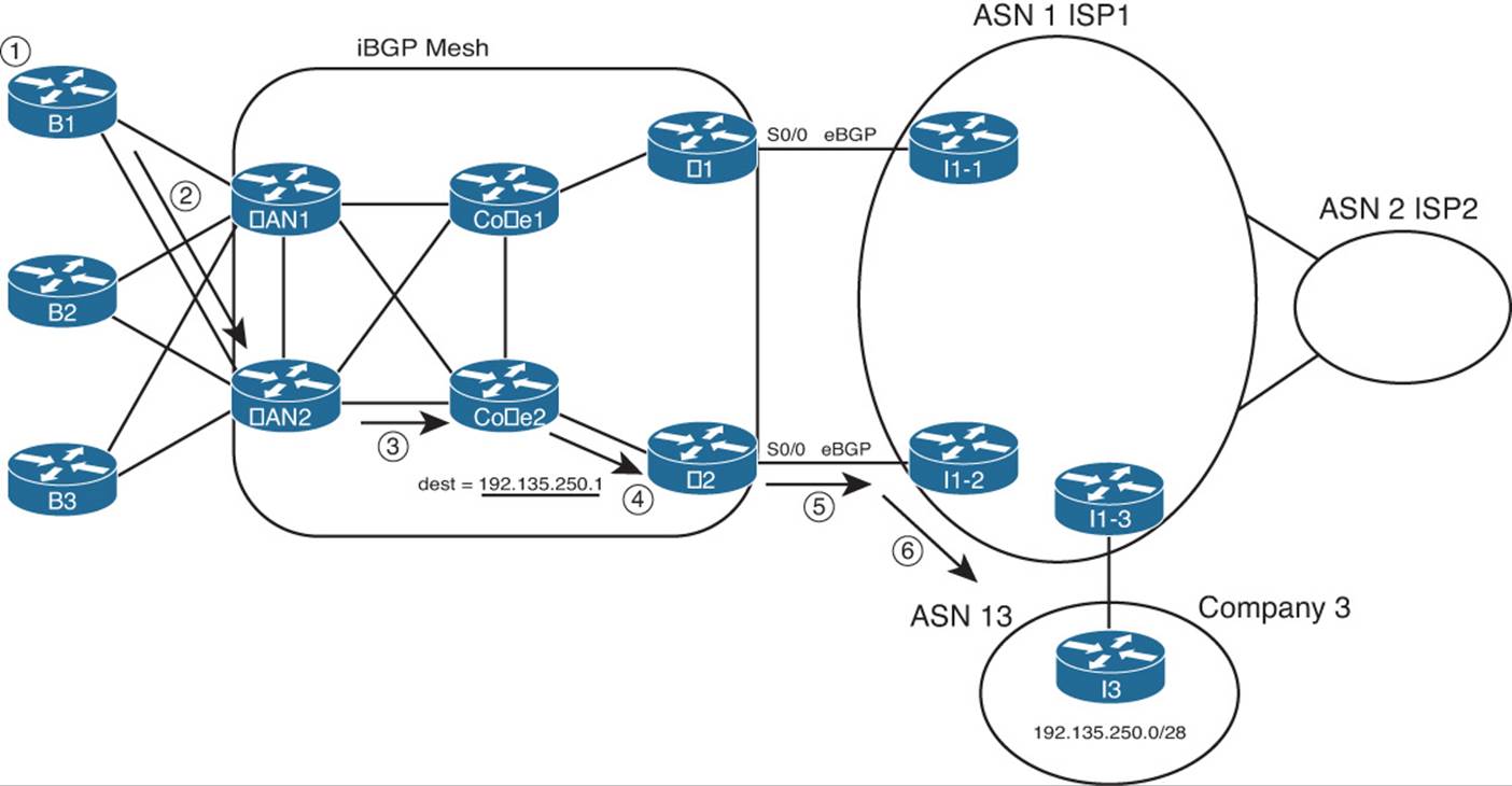
Figure 13-11 Preferring One Outbound Link over Another
Two notable actions must take place for this design to work, beyond the basic configuration of the eBGP peers as shown. First, the engineers at the enterprise and ISP must agree on to how to make BGP specify a prefix as being best reached through a particular link. In this case, the routes advertised by I1-2 for prefix for 192.135.250.0/28 must have BGP PA settings that appear better than those learned from I1-1. In this case, you cannot just rely on the default of checking the AS_PATH length, because the AS_PATH length should tie, because I1-1 and I1-2 are in the same ASN. So when planning with the engineers of ISP1, the enterprise network engineer must discuss what kinds of prefixes that might work better through I1-1, which would be better through I1-2, and how the ISP might set PA values to which the enterprise routers (E1 and E2) can react.
The second big consideration occurs inside the enterprise network with a need to run BGP between multiple routers. So far in this chapter, the enterprise routers all used default routes to send packets to the Internet-facing routers, and only those routers knew Internet routes. However, for the design of Figure 13-11 to work, E1 and E2 must communicate BGP routes using an iBGP connection. And because packet forwarding between E1 and E2 goes through other routers (such as Core1 and Core2), those routers typically also need to run BGP. You might even decide to run BGP on the WAN routers as well. By doing so, the core routers know the best BGP routes. For example, they all know that the better route for Company 3’s 192.135.250.0/28 public address space is through E2, so the packet is forwarded to E2. The following list outlines the logic matching Figure 13-11:
Step 1. A host at Branch B1 sends a packet to 192.135.250.1.
Step 2. Router B1 matches its default route, forwarding the packet to Router WAN2.
Step 3. WAN2 matches its iBGP-learned route for 192.135.250.0/28, forwarding to Core2.
Step 4. Core2 matches its iBGP-learned route for 192.135.250.0/28, forwarding to E2.
Step 5. E2 matches its eBGP-learned route for 192.135.250.0/28, forwarding to I1-2.
Step 6. The routers in ISP1 forward the packet to Router I3, in Company 3.
The routers in the core of the enterprise need to run BGP, because without it, routing loops can occur. For example, if WAN1, WAN2, Core1, and Core2 did not use BGP, and relied on default routes, their default would drive packets to either E1 or E2. Then, E1 or E2 might send the packets right back to Core1 or Core2. (Note that there is no direct link between E1 and E2.) Figure 13-12 shows just such a case.
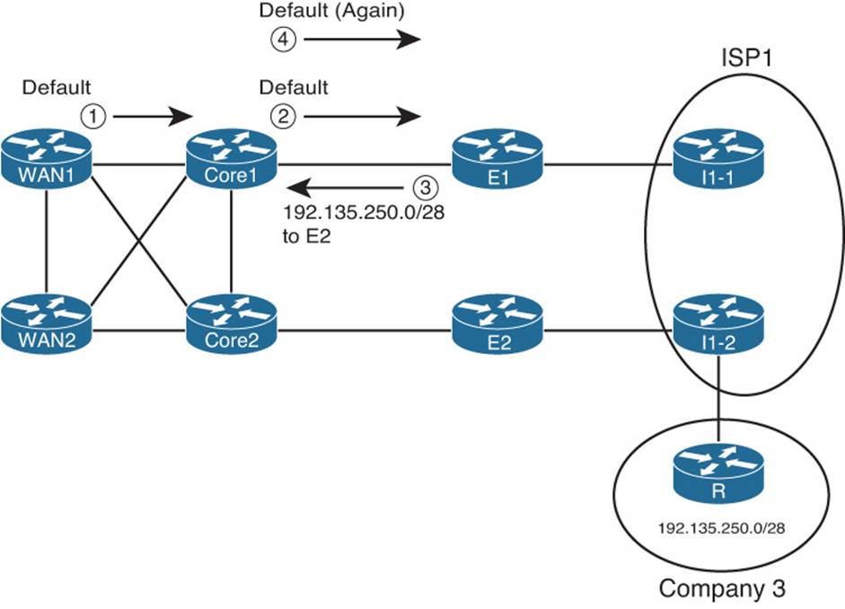
Figure 13-12 Routing Loop Without BGP in the Enterprise Core
In this case, both E1 and E2 know that E2 is the best exit point for packets destined to 192.135.250.0/28 (from Figure 13-11). However, the core routers use default routes, with WAN1 and Core1 using defaults that send packets to E1. Following the numbers in the figure:
Step 1. WAN1 gets a packet destined for 192.135.250.1 and forwards the packet to Core1 based on its default route.
Step 2. Core1 gets the packet and has no specific route, so it forwards the packet to E1 based on its default route.
Step 3. E1’s BGP route tells it that E2 is the better exit point for this destination. To send the packet to E2, E1 forwards the packet to Core1.
Step 4. Core1, with no knowledge of the BGP route for 192.135.250.0/28, uses its default route to forward the packet to E1, so the packet is now looping.
A mesh of iBGP peerings between at least E1, E2, Core1, and Core2 would prevent this problem.
Partial and Full BGP Updates
Unfortunately, enterprise routers must pay a relatively large price for the ability to choose between competing BGP routes to reach Internet destinations. As previously mentioned, the BGP table in the Internet core is at approximately 480,000 routes as of the writing of this chapter in 2014. To make a decision to use one path instead of another, an enterprise router must know about at least some of those routes. Exchanging BGP information for such a large number of routes consumes bandwidth. It also consumes memory in the routers and requires some processing to choose the best routes. Some samples at Cisco.com show BGP using approximately 70 MB of RAM for the BGP table on a router with 100,000 BGP-learned routes.
To make matters a bit worse, in some cases, several enterprise routers might also need to use BGP, as shown in the previous section. Those routers also need more memory to hold the BGP table, and they consume bandwidth exchanging the BGP table.
To help reduce the memory requirements of receiving full BGP updates (BGP updates that include all routes), some ISPs give you three basic options for what routes the ISP advertises:
![]() Default route only: The ISP advertises a default route with BGP, but no other routes.
Default route only: The ISP advertises a default route with BGP, but no other routes.
![]() Full updates: The ISP sends you the entire BGP table.
Full updates: The ISP sends you the entire BGP table.
![]() Partial updates: The ISP sends you routes for prefixes that might be better reached through that ISP, but not all routes, plus a default route (to use as needed instead of the purposefully omitted routes).
Partial updates: The ISP sends you routes for prefixes that might be better reached through that ISP, but not all routes, plus a default route (to use as needed instead of the purposefully omitted routes).
If all you want to do with a BGP connection is use it by default, you can have the ISP send just a default route. If you are willing to take on the overhead of getting all BGP routes, asking for full updates is reasonable. However, if you want something in between, the partial updates option is useful.
BGP partial updates give you the benefit of choosing the best routes for some destinations, while limiting the bandwidth and memory consumption. With partial updates, the ISP advertises routes for prefixes that truly are better reached through a particular link. However, for prefixes that might not be any better through that link, the ISP does not advertise those prefixes with BGP. Then the enterprise routers can use the better path based on the routes learned with BGP, and use a default route for the prefixes not learned with BGP. For example, previously in Figure 13-11, Router I1-2 could be configured to only advertise routes for those such as 192.135.250.0/28 from Company 3 in that figure—in other words, only routes for which Router I1-2 had a clearly better route than the other ISP1 routers.
Single-Multihomed
A single-multihomed topology means a single link per ISP, but multiple (at least two) ISPs. Figure 13-13 shows a couple of single-multihomed designs, each with two ISPs.
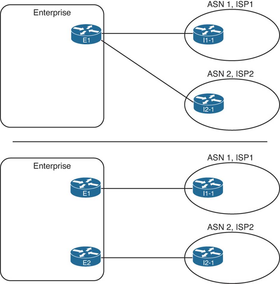
Figure 13-13 Single-Multihomed Designs
The single-multihomed design has some similarities with both the single-homed and dual-homed designs previously seen in this section. The single-multihomed design on the top of the figure, which uses a single router, acts like the single-homed design for default routes in the enterprise. This design can flood a default route throughout the enterprise, drawing traffic to that one router, because only one router connects to the Internet. With the two-router design on the lower half of Figure 13-13, default routes can still be used in the enterprise to draw traffic to the preferred Internet connection (if one is preferred) or to balance traffic across both.
The single-multihomed design works like the dual-homed design in some ways, because two (or more) links connect the enterprise to the Internet. With two links, the Internet design might call for the use of defaults, always preferring one of the links. The design engineer might also choose to use BGP, learn either full or partial updates, and then favor one connection over another for some of the routes.
Figure 13-14 shows these concepts with a single-multihomed design, with default routes in the enterprise to the one Internet router (E1).
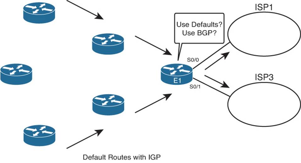
Figure 13-14 Outbound Routing with a Single-Multihomed Design
Dual-Multihomed
The last general category of Internet access topologies is called dual-multihomed. With this design, two or more ISPs are used, with two or more connections to each. A number of different routers can be used. Figure 13-15 shows several examples.
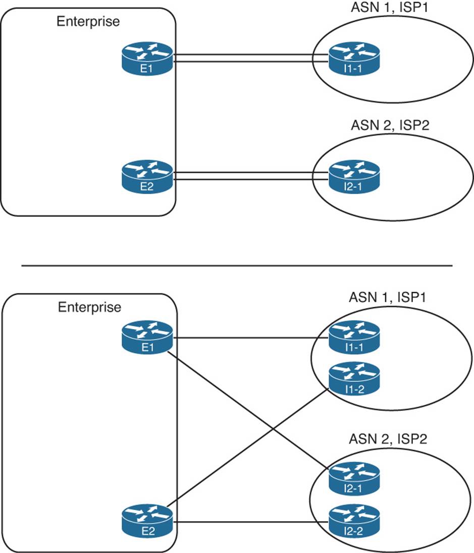
Figure 13-15 Dual-Multihomed Options
Figure 13-15 does not show all design options, but because at least two ISPs exist, with at least two connections per ISP, much redundancy exists. That redundancy can be used for backup, but most often, BGP is used to make some decisions about the best path to reach various destinations.
External BGP for Enterprises
Some of the core operational concepts of BGP mirror those of EIGRP and OSPF. BGP first forms a neighbor relationship with peers. BGP then learns information from its neighbors, placing that information in a table—the BGP table. Finally, BGP analyzes the BGP table to choose the best working route for each prefix in the BGP table, placing those routes into the IP routing table.
This section discusses external BGP (eBGP), focusing on two of the three aspects of how a routing protocol learns routes: forming neighborships and exchanging the reachability or topology information that is stored in the BGP table. First, this section examines the baseline configuration ofeBGP peers (also called neighbors), along with several optional settings that might be needed specifically for eBGP connections. This configuration should result in working BGP neighborships. Then, this section examines the BGP table, listing the prefix/length and path attributes (PA) learned from the Internet, and the IP routing table.
eBGP Neighbor Configuration
At a minimum, a router participating in BGP must configure the following settings:
![]() The router’s own ASN (router bgp asn global command)
The router’s own ASN (router bgp asn global command)
![]() The IP address of each neighbor and that neighbor’s ASN (neighbor ip-address remote-as remote-asn BGP subcommand)
The IP address of each neighbor and that neighbor’s ASN (neighbor ip-address remote-as remote-asn BGP subcommand)
For example, consider a typical multihomed enterprise Internet design, as shown in Figure 13-16. In this case, the following design requirements have already been decided, but you must then determine the configuration, knowing the information in the following list and the figure:
![]() The enterprise uses ASN 11.
The enterprise uses ASN 11.
![]() The connection to ISP1 (two T-1s) is considered the primary connection, with the connection to ISP3 (one T-1) being secondary.
The connection to ISP1 (two T-1s) is considered the primary connection, with the connection to ISP3 (one T-1) being secondary.
![]() ISP1 advertises a default route, plus full updates.
ISP1 advertises a default route, plus full updates.
![]() ISP1 uses ASN 1.
ISP1 uses ASN 1.
![]() ISP3 advertises a default route, plus partial updates that include only ISP3’s local customers.
ISP3 advertises a default route, plus partial updates that include only ISP3’s local customers.
![]() ISP3 uses ASN 3.
ISP3 uses ASN 3.
![]() Each ISP uses the IP address of its lowest-numbered interface for its peer relationships.
Each ISP uses the IP address of its lowest-numbered interface for its peer relationships.
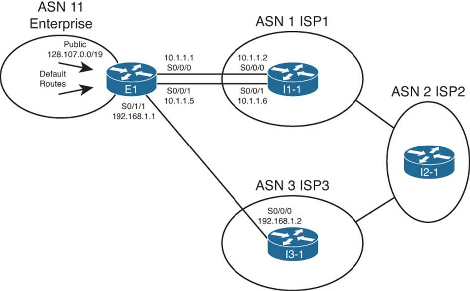
Figure 13-16 Sample Single-Multihomed Design
For Router E1, as shown in Example 13-2, the BGP configuration requires only three commands, at least to configure BGP to the point where E1 will form neighborships with the two other routers. (Note that this chapter continues to change and add to this configuration when introducing new concepts.) The example also shows the configuration on Routers I1-1 and I3-1 added solely to support the neighbor connections to E1; other BGP configuration on these routers is not shown.
Example 13-2 BGP Configuration on E1: Neighborships Configured
! Configuration on router E1
router bgp 11
neighbor 10.1.1.2 remote-as 1
neighbor 192.168.1.2 remote-as 3
! Next commands are on I1-1
router bgp 1
neighbor 10.1.1.1 remote-as 11
! Next commands are on I3-1
router bgp 3
neighbor 192.168.1.1 remote-as 11
The gray portions of the output highlight the configuration of the local ASN and the neighbors’ ASNs—parameters that must match for the neighborships to form. First, E1 configures its own ASN as 11 by using the router bgp 11 command. The other routers must refer to ASN 11 on the neighbor commands that refer to E1; in this case, I1-1 refers to ASN 11 with its neighbor 10.1.1.1 remote-as 11 command. Conversely, I1-1’s local ASN (1) on its router bgp 1 global command must match what E1 configures in a neighbor command—in this case, with E1’s neighbor 10.1.1.2 remote-as 1 command.
Requirements for Forming eBGP Neighborships
Routers must meet several requirements to become BGP neighbors:
![]() A local router’s ASN (on the router bgp asn command) must match the neighboring router’s reference to that ASN with its neighbor remote-as asn command.
A local router’s ASN (on the router bgp asn command) must match the neighboring router’s reference to that ASN with its neighbor remote-as asn command.
![]() The BGP router IDs of the two routers must not be the same.
The BGP router IDs of the two routers must not be the same.
![]() If configured, authentication must pass.
If configured, authentication must pass.
![]() Each router must be part of a TCP connection with the other router, with the remote router’s IP address used in that TCP connection matching what the local router configures in a BGP neighbor remote-as command.
Each router must be part of a TCP connection with the other router, with the remote router’s IP address used in that TCP connection matching what the local router configures in a BGP neighbor remote-as command.
Consider the first two items in this list. First, the highlights in Example 13-2 demonstrate the first of the four requirements. Next, the second requirement in the list requires only a little thought if you recall the similar details about router IDs (RID) with EIGRP and OSPF. Like EIGRP and OSPF, BGP defines a 32-bit router ID, written in dotted-decimal notation. And like EIGRP and OSPF, BGP on a router chooses its RID the same general way, by using the following steps, in order, until a BGP RID has been chosen:
![]() Configured: Use the setting of the bgp router-id rid router subcommand.
Configured: Use the setting of the bgp router-id rid router subcommand.
![]() Highest loopback: Choose the highest numeric IP address of any up loopback interface, at the time the BGP process initializes.
Highest loopback: Choose the highest numeric IP address of any up loopback interface, at the time the BGP process initializes.
![]() Highest other interface: Choose the highest numeric IP address of any up nonloopback interface, at the time the BGP process initializes.
Highest other interface: Choose the highest numeric IP address of any up nonloopback interface, at the time the BGP process initializes.
The third requirement in the list, the authentication check, occurs only if authentication has been configured on at least one of the two routers, using the neighbor neighbor-ip password key command. If two BGP neighbors configure this command, referring to the other routers’ IP address, while configuring a matching authentication key value, the authentication passes. If both omit this command, no authentication occurs. However, the neighborship can still form. If the keys do not match, or if only one router configures authentication, authentication fails, resulting in no neighborship forming.
The fourth neighbor requirement—that the IP addresses used for the neighbor TCP connection match—requires a more detailed discussion. BGP neighbors first form a TCP connection. Later, BGP messages flow over that connection, which allows BGP routers to know when the messages arrived at the neighbor and when they did not.
A BGP router creates the TCP connection by trying to establish a TCP connection to the address configured in the neighbor neighbor-ip remote-as command. However, Cisco IOS does not require the BGP configuration to explicitly state the source address that router uses when establishing this TCP connection, and if not explicitly configured, Cisco IOS picks an IP address on the local router. By default, Cisco IOS chooses its BGP source IP address for a given neighbor as the interface IP address of the outgoing interface of the route used to forward packets to that neighbor. That’s a lot of words to fight through, and much more easily seen with a figure, such as Figure 13-17, which focuses on the eBGP connection between E1 and I1-1 shown in Figure 13-16.
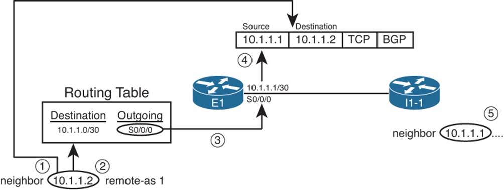
Figure 13-17 Default Choice for Update Source
A description of the steps in the logic shown in the figure follows:
Step 1. E1 finds the neighbor 10.1.1.2 command, so E1 sends the BGP messages for this neighbor inside packets with destination IP address 10.1.1.2.
Step 2. E1 looks in the IP routing table for the route that matches destination 10.1.1.2.
Step 3. The route matched in Step 2 lists S0/0/0 as the outgoing interface.
Step 4. E1’s interface IP address for S0/0/0 is 10.1.1.1, so E1 uses 10.1.1.1 as its source IP address for this BGP peer.
Step 5. The neighbor command on the other router, I1-1, must refer to E1’s source IP address (10.1.1.1 in this case).
Now, consider again the last of the four requirements to become neighbors. Restated, for proper operation, the BGP update source on one router must match the IP address configured on the other router’s neighbor command, and vice versa. As shown in Figure 13-14, E1 uses update source 10.1.1.1, with I1-1 configuring the neighbor 10.1.1.1 command. Conversely, I1-1 uses 10.1.1.2 as its update source for this neighbor relationship, with E1 configuring a matching neighbor 10.1.1.2 command.
Note
The update source concept applies per neighbor.
Issues When Redundancy Exists Between eBGP Neighbors
In many cases, a single Layer 3 path exists between eBGP neighbors. For example, a single T1, or single T3, or maybe a single MetroE Virtual Private Wire Service (VPWS) path exists between the two routers. In such cases, the eBGP configuration can simply use the interface IP addresses on that particular link. For example, in Figure 13-16, a single serial link exists between Routers E1 and I3-1, and they can reasonably use the serial link’s IP addresses, as shown in Example 13-2.
However, when redundant Layer 3 paths exist between two eBGP neighbors, the use of interface IP addresses for the underlying TCP connection can result in an outage when only one of the two links fails. BGP neighborships fail when the underlying TCP connection fails. TCP uses a concept called a socket, which consists of a local TCP port number and an IP address. That IP address must be associated with a working interface (an interface whose state is line status up, line protocol up, per the show interfaces command). If the interface whose IP address is used by BGP were to fail, the TCP socket would fail, closing the TCP connection. As a result, the BGP neighborship can only be up when the associated interface also happens to be up.
Two alternative solutions exist in this case. One option would be to configure two neighbor commands on each router, one for each of the neighbor’s interface IP addresses. This solves the availability issue, because if one link fails, the other neighborship can remain up and working. However, in this case, both neighborships exchange BGP routes, consuming bandwidth and more memory in the BGP table.
The preferred option, which uses loopback interfaces as the TCP connection endpoints, solves the availability problem while avoiding the extra overhead. The two routers each configure a loopback interface and IP address, and use those loopback IP addresses as the source of their single BGP TCP connection. If one of the multiple links fails, the loopback interface does not fail. As long as the two routers have working routes to reach each other’s loopback IP addresses, the TCP connection does not fail.
Configuring eBGP peers to use a loopback interface IP address with BGP requires several steps, as follows:
Step 1. Configure an IP address on a loopback interface on each router.
Step 2. Tell BGP on each router to use the loopback IP address as the source IP address using the neighbor neighbor-ip update-source interface-id command.
Step 3. Configure the BGP neighbor command on each router to refer to the other router’s loopback IP address at the neighbor IP address in the neighbor neighbor-ip remote-as command.
Step 4. Make sure that each router has IP routes so that they can forward packets to the loopback interface IP address of the other router.
Step 5. Configure eBGP multihop using the neighbor neighbor-ip ebgp-multihop hops command.
The first three steps in the list require configuration on both the routers. Figure 13-18 shows the details related to the first three steps, focusing on Router E1’s use of its Loopback1 interface (based on Figure 13-16).
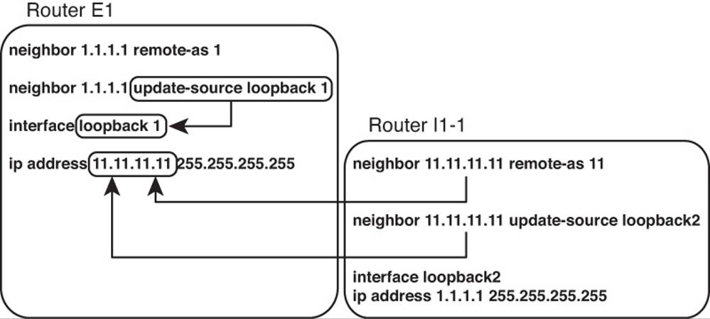
Figure 13-18 Using Loopbacks with Update Source for eBGP
The fourth step in the list is an overt reminder that for TCP to work, both routers must be able to deliver packets to the IP address listed in the neighbor commands. Because the neighbor commands now refer to loopback IP addresses, the routers cannot rely on connected routes for forwarding the packets. To give each router a route to the other router’s loopback, you can run an instance of an IGP to learn the routes, or just configure static routes. If using static routes, make sure to configure the routes so that all redundant paths would be used (as seen in the upcomingExample 13-3). If using an IGP, make sure that the configuration allows the two routers to become IGP neighbors over all redundant links as well.
eBGP Multihop Concepts
The fifth configuration step for using loopback IP addresses with eBGP peers refers to a feature called eBGP multihop. By default, when building packets to send to an eBGP peer, Cisco IOS sets the IP Time-To-Live (TTL) field in the IP header to a value of 1. With this default action, the eBGP neighborship fails to complete when using loopback interface IP addresses. The reason is that when the packet with TTL=1 arrives at the neighbor, the neighbor decrements the TTL value to 0 and discards the packet.
The logic of discarding the BGP packets can be a bit surprising, so an example can help. For this example, assume that the default action of TTL=1 is used and that eBGP multihop is not configured yet. Router E1 from Figure 13-16 is trying to establish a BGP connection to I1-1, using I1-1’s loopback IP address 1.1.1.1, as shown in Figure 13-18. The following occurs with the IP packets sent by E1 when attempting to form a TCP connection for BGP to use:
Step 1. E1 sends a packet to destination address 1.1.1.1, TTL=1.
Step 2. I1-1 receives the packet. Seeing that the packet is not destined for the receiving interface’s IP address, I1-1 passes the packet off to its own IP forwarding (IP routing) logic.
Step 3. I1-1’s IP routing logic matches the destination (1.1.1.1) with the routing table and finds interface loopback 2 as the outgoing interface.
Step 4. I1-1’s IP forwarding logic decrements the TTL by 1, decreasing the TTL to 0, and as a result, I1-1 discards the packet.
In short, the internal Cisco IOS packet-forwarding logic decrements the TTL before giving the packet to the loopback interface, meaning that the normal IP forwarding logic discards the packet.
Configuring the routers with the neighbor ebgp-multihop 2 command, as seen in the upcoming Example 13-3, solves the problem. This command defines the TTL that the router will use when creating the BGP packets (two in this case). As a result, the receiving router will decrement the TTL to 1, so the packet will not be discarded.
BGP Internals and Verifying eBGP Neighbors
Similar to OSPF, the BGP neighbor relationship goes through a series of states over time. Although the Finite State Machine (FSM) for BGP neighbor states has many twists and turns, particularly for handling exceptions, retries, and failures, the overall process works as follows:
Step 1. A router tries to establish a TCP connection with the IP address listed on a neighbor command, using well-known destination port 179.
Step 2. When the three-way TCP connection completes, the router sends its first BGP message, the BGP Open message, which generally performs the same function as the EIGRP and OSPF Hello messages. The Open message contains several BGP parameters, including those that must be verified before allowing the routers to become neighbors.
Step 3. After an Open message has been sent and received and the neighbor parameters match, the neighbor relationship is formed and the neighbors reach the Established state.
Table 13-6 lists the various BGP states. If all works well, the neighborship reaches the final state: Established. When the neighbor relationship (also called a BGP peer or BGP peer connection) reaches the Established state, the neighbors can send BGP Update messages, which list PAs and prefixes. However, if neighbor relationship fails for any reason, the neighbor relationship can cycle through all the states listed in Table 13-6 while the routers periodically attempt to bring up the neighborship.
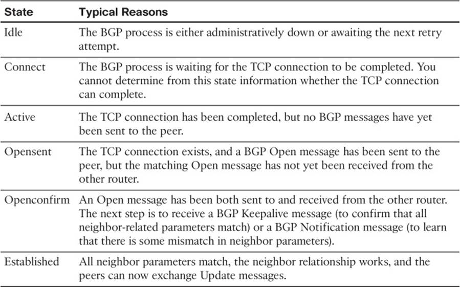
Table 13-6 BGP Neighbor States
Verifying eBGP Neighbor Status
The two most common commands to display a BGP neighbor’s status are show ip bgp summary and show ip bgp neighbors [neighbor-id]. Interestingly, most people use the first of these commands, because it supplies a similar amount of information, one line per neighbor, as do the familiar show ip eigrp neighbors and show ip ospf neighbor commands. The show ip bgp neighbors command lists a large volume of output per neighbor, which, although useful, usually contains far too much information for the verification of the current neighbor state. Examples 13-3and 13-4 show samples of the output of each of these two commands on Router E1, respectively, based on the configuration shown in Example 13-2, with some description following each example.
Example 13-3 Summary Information with the show ip bgp summary Command
E1# show ip bgp summary
BGP router identifier 11.11.11.11, local AS number 11
BGP table version is 26, main routing table version 26
6 network entries using 792 bytes of memory
7 path entries using 364 bytes of memory
6/4 BGP path/bestpath attribute entries using 888 bytes of memory
5 BGP AS-PATH entries using 120 bytes of memory
0 BGP route-map cache entries using 0 bytes of memory
0 BGP filter-list cache entries using 0 bytes of memory
Bitfield cache entries: current 1 (at peak 2) using 32 bytes of memory
BGP using 2196 total bytes of memory
BGP activity 12/6 prefixes, 38/31 paths, scan interval 60 secs
Neighbor V AS MsgRcvd MsgSent TblVer InQ OutQ Up/Down State/PfxRcd
1.1.1.1 4 1 60 61 26 0 0 00:45:01 6
192.168.1.2 4 3 153 159 26 0 0 00:38:13 1
The first line in the summary lists the local router’s BGP RID (11.11.11.11), along with the local router’s ASN (11). The rest of the summary focuses on statistics for the BGP table entries. The bottom of the output lists a heading line (highlighted in the output), plus one line per neighbor, with two neighbors in this case. The Neighbor column lists the IP address as defined on the local router’s neighbor command and not the neighbor’s BGP RID. Other notable information includes the neighbor’s ASN (as configured on the local router’s neighbor remote-as command), the time spent in the current state, and an interesting heading: State/PfxRcd.
This State/PfxRcd heading either lists the BGP neighbor state, as summarized in Table 13-6, or the number of prefixes received (PfxRcd) from that neighbor. A numeric value under this heading implies a neighbor state of Established, because the peers must be in the Established state before Updates can be sent. If the peer is not in an Established state, the value in this heading lists the text name of the current BGP state.
Example 13-4 shows a sample of the show ip bgp neighbors 1.1.1.1 command on Router E1, which displays information about the connection to Router I1-1 in Figure 13-16. This command lists several facts not seen in the shorter show ip bgp summary command output in Example 13-3. The example highlights some of those key items, with the following comments referring to those highlighted items, in order:
![]() The neighbor is an eBGP neighbor (external link).
The neighbor is an eBGP neighbor (external link).
![]() The neighbor’s BGP RID (1.1.1.1).
The neighbor’s BGP RID (1.1.1.1).
![]() The current state (Established) is explicitly listed.
The current state (Established) is explicitly listed.
![]() Route refresh is enabled.
Route refresh is enabled.
![]() The eBGP multihop setting (two hops).
The eBGP multihop setting (two hops).
![]() Local and remote TCP socket information (IP addresses and port numbers).
Local and remote TCP socket information (IP addresses and port numbers).
Example 13-4 Detailed Information with the show ip bgp neighbors Command
E1# show ip bgp neighbors 1.1.1.1
BGP neighbor is 1.1.1.1, remote AS 1, external link
BGP version 4, remote router ID 1.1.1.1
BGP state = Established, up for 00:45:08
Last read 00:00:02, last write 00:00:38, hold time is 180, keepalive interval is
60 seconds
Neighbor capabilities:
Route refresh: advertised and received(new)
Address family IPv4 Unicast: advertised and received
Message statistics:
InQ depth is 0
OutQ depth is 0
Sent Rcvd
Opens: 2 2
Notifications: 0 0
Updates: 16 12
Keepalives: 43 47
Route Refresh: 0 0
Total: 61 61
Default minimum time between advertisement runs is 30 seconds
For address family: IPv4 Unicast
BGP table version 26, neighbor version 26/0
Output queue size : 0
Index 1, Offset 0, Mask 0x2
1 update-group member
Sent Rcvd
Prefix activity: ---- ----
Prefixes Current: 6 6 (Consumes 312 bytes)
Prefixes Total: 19 7
Implicit Withdraw: 11 0
Explicit Withdraw: 2 1
Used as bestpath: n/a 5
Used as multipath: n/a 0
Outbound Inbound
Local Policy Denied Prefixes: ---- ----
AS_PATH loop: n/a 2
Total: 0 2
Number of NLRIs in the update sent: max 3, min 1
Address tracking is enabled, the RIB does have a route to 1.1.1.1
Connections established 2; dropped 1
Last reset 00:45:10, due to Peer closed the session
External BGP neighbor may be up to 2 hops away.
Transport(tcp) path-mtu-discovery is enabled
Connection state is ESTAB, I/O status: 1, unread input bytes: 0
Connection is ECN Disabled, Minimum incoming TTL 0, Outgoing TTL 2
Local host: 11.11.11.11, Local port: 179
Foreign host: 1.1.1.1, Foreign port: 28995
Connection tableid (VRF): 0
Enqueued packets for retransmit: 0, input: 0 mis-ordered: 0 (0 bytes)
Event Timers (current time is 0x8217A0):
Timer Starts Wakeups Next
Retrans 49 0 0x0
TimeWait 0 0 0x0
AckHold 49 46 0x0
SendWnd 0 0 0x0
KeepAlive 0 0 0x0
GiveUp 0 0 0x0
PmtuAger 0 0 0x0
DeadWait 0 0 0x0
Linger 0 0 0x0
ProcessQ 0 0 0x0
iss: 2070882650 snduna: 2070884280 sndnxt: 2070884280 sndwnd: 15890
irs: 3327995414 rcvnxt: 3327996693 rcvwnd: 16156 delrcvwnd: 228
SRTT: 300 ms, RTTO: 306 ms, RTV: 6 ms, KRTT: 0 ms
minRTT: 0 ms, maxRTT: 300 ms, ACK hold: 200 ms
Status Flags: passive open, gen tcbs
Option Flags: nagle, path mtu capable, md5
IP Precedence value : 6
Datagrams (max data segment is 516 bytes):
Rcvd: 98 (out of order: 0), with data: 50, total data bytes: 1278
Sent: 99 (retransmit: 0, fastretransmit: 0, partialack: 0, Second Congestion: 0),
with data: 50, total data bytes: 1629
Packets received in fast path: 0, fast processed: 0, slow path: 0
fast lock acquisition failures: 0, slow path: 0
E1# show tcp brief
TCB Local Address Foreign Address (state)
66D27FE0 192.168.1.1.179 192.168.1.2.16489 ESTAB
66D27378 11.11.11.11.179 1.1.1.1.28995 ESTAB
Note that the end of the example shows another command that you can use to confirm the TCP socket details of the underlying TCP connection: show tcp brief.
Administratively Controlling Neighbor Status
Interestingly, Cisco IOS provides a means by which network operations personnel can administratively disable any BGP neighbor. To do so, the operator would enter BGP configuration mode and issue the neighbor neighbor-ip shutdown command. This command brings down the current neighbor to an idle state. Later, when the BGP connection should be brought up, the operator should repeat the process, but with the no version of the command (no neighbor neighbor-ip shutdown).
These commands can be particularly useful to try in a lab when learning BGP. Teamed with the debug ip bgp command, you can bring down neighbors and see the somewhat-readable BGP messages. These messages list the BGP states from Table 13-6. They also show the information inside the Open messages. Example 13-5 shows a sample, with the debug messages that note a state transition highlighted. The output also lists the show ip bgp summary command output, with the administratively idle state created by the neighbor 1.1.1.1 shutdown BGP configuration command on Router E1.
Example 13-5 BGP Shutdown and BGP Neighbor State Transitions
E1# debug ip bgp
BGP debugging is on for address family: IPv4 Unicast
E1# conf t
Enter configuration commands, one per line. End with CNTL/Z.
E1(config)# router bgp 11
E1(config-router)# neighbor 1.1.1.1 shutdown
E1(config-router)#
*Aug 11 20:23:01.335: BGPNSF state: 1.1.1.1 went from nsf_not_active to nsf_not_
active
*Aug 11 20:23:01.335: BGP: 1.1.1.1 went from Established to Idle
*Aug 11 20:23:01.335: %BGP-5-ADJCHANGE: neighbor 1.1.1.1 Down Admin. Shutdown
E1(config-router)# do show ip bgp summary
! lines omitted for brevity
Neighbor V AS MsgRcvd MsgSent TblVer InQ OutQ Up/Down State/PfxRcd
1.1.1.1 4 1 87 87 0 0 0 00:00:06 Idle (Admin)
192.168.1.2 4 3 173 183 41 0 0 00:58:47 1
E1(config-router)# no neighbor 1.1.1.1 shutdown
E1(config-router)#
*Aug 11 20:23:26.571: BGP: 1.1.1.1 went from Idle to Active
*Aug 11 20:23:26.571: BGP: 1.1.1.1 open active, local address 11.11.11.11
*Aug 11 20:23:26.575: BGP: 1.1.1.1 read request no-op
*Aug 11 20:23:26.575: BGP: 1.1.1.1 went from Active to OpenSent
*Aug 11 20:23:26.575: BGP: 1.1.1.1 sending OPEN, version 4, my as: 11, holdtime 180
seconds
*Aug 11 20:23:26.579: BGP: 1.1.1.1 send message type 1, length (incl. header) 45
*Aug 11 20:23:26.583: BGP: 1.1.1.1 rcv message type 1, length (excl. header) 26
*Aug 11 20:23:26.587: BGP: 1.1.1.1 rcv OPEN, version 4, holdtime 180 seconds
*Aug 11 20:23:26.587: BGP: 1.1.1.1 rcv OPEN w/ OPTION parameter len: 16
*Aug 11 20:23:26.587: BGP: 1.1.1.1 rcvd OPEN w/ optional parameter type 2
(Capability) len 6
*Aug 11 20:23:26.587: BGP: 1.1.1.1 OPEN has CAPABILITY code: 1, length 4
*Aug 11 20:23:26.587: BGP: 1.1.1.1 OPEN has MP_EXT CAP for afi/safi: 1/1
*Aug 11 20:23:26.587: BGP: 1.1.1.1 rcvd OPEN w/ optional parameter type 2
(Capability) len 2
*Aug 11 20:23:26.587: BGP: 1.1.1.1 OPEN has CAPABILITY code: 128, length 0
*Aug 11 20:23:26.587: BGP: 1.1.1.1 OPEN has ROUTE-REFRESH capability(old) for all
address-families
*Aug 11 20:23:26.587: BGP: 1.1.1.1 rcvd OPEN w/ optional parameter type 2
(Capability) len 2
*Aug 11 20:23:26.587: BGP: 1.1.1.1 OPEN has CAPABILITY code: 2, length 0
*Aug 11 20:23:26.587: BGP: 1.1.1.1 OPEN has ROUTE-REFRESH capability(new) for all
address-families
BGP: 1.1.1.1 rcvd OPEN w/ remote AS 1
*Aug 11 20:23:26.587: BGP: 1.1.1.1 went from OpenSent to OpenConfirm
*Aug 11 20:23:26.591: BGP: 1.1.1.1 went from OpenConfirm to Established
*Aug 11 20:23:26.591: %BGP-5-ADJCHANGE: neighbor 1.1.1.1 Up
*Aug 11 20:23:26.603: BGP_Router: unhandled major event code 128, minor 0
BGP Message Summary
So far, this chapter has mentioned three of the four BGP messages. For reference, Table 13-7 lists the four BGP messages, with comparisons to EIGRP messages for perspective.
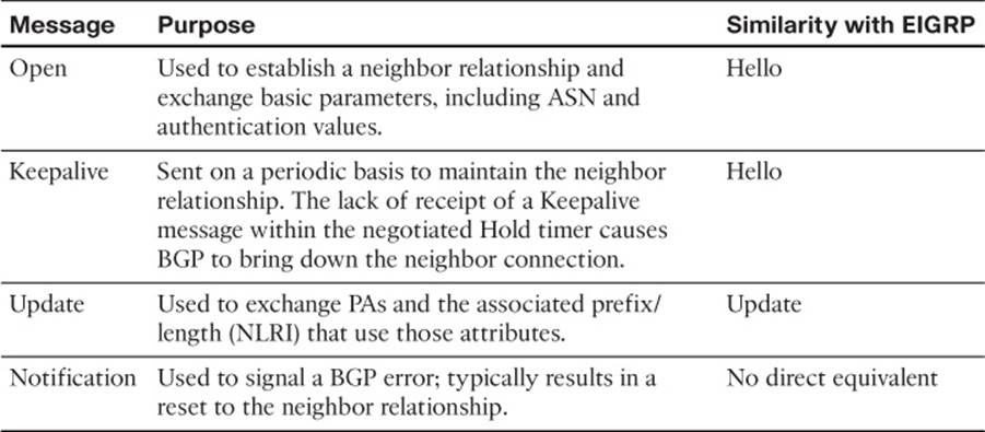
Table 13-7 BGP Message Types
Verifying the BGP Table
When an enterprise router has established its eBGP neighbor relationships, that router can advertise and learn routes using BGP. To learn routes, an enterprise BGP router does not need additional configuration beyond the configuration of eBGP neighbors, as discussed earlier. To advertise routes to eBGP peers, particularly the public IP address prefix(es) used by that enterprise, the enterprise BGP router needs some additional configuration, as discussed in the upcoming section “Injecting Routes into BGP for Advertisement to the ISPs.”
The BGP table plays a key role in the process of learning and using routing information with BGP. A router stores all learned BGP prefixes and PAs in its BGP table. The router will later choose which route for each prefix is the best BGP route. The router can then advertise its BGP table to its neighbors, advertising only the best route for each prefix.
This section begins with a brief examination of the BGP Update process by which BGP neighbors exchange routing information. Next, the text looks at the various show commands that can be used to examine and confirm the contents of the BGP table.
The BGP Update Message
When a BGP neighborship reaches the Established state, those neighbors begin sending BGP Update messages to each other. The router receiving an Update places those learned prefixes into its BGP table, regardless of whether the route appears to be the best route. Like EIGRP and OSPF, BGP puts all learned routing information into its table, and then BGP processes all such potential routes to choose the best route for each prefix.
The BGP Update message itself can be revealing about the motivations behind BGP. Figure 13-19 shows the format of the Update message.
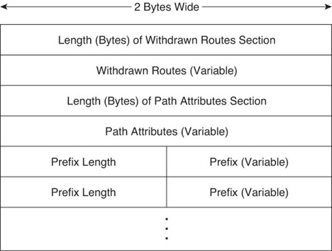
Figure 13-19 Format of the BGP Update Message
Interestingly, the format of the Update message tells us something about the nature of BGP as a Path Vector algorithm. The message lists a set of PAs and then a potentially long list of prefixes that use that set of PAs. So, you might view the BGP Update message as focusing on advertising paths, or a set of PAs, along with the associated list of prefixes that use the advertised path. Because BGP uses the information in the combined set of PAs to make a decision of which path is best, its underlying logic is called path vector.
BGP uses the Update message to both announce and withdraw routes. For example, when a router realizes that a route in the router’s BGP table has failed, that router withdraws that route by sending a BGP Update to its neighbors, listing the prefix in the list of withdrawn routes. When a router receives an Update that lists a prefix as withdrawn, that router knows that the route has failed. (Note the field near the top of the Update message that lists withdrawn routes.) That same Update message might contain other announced prefixes later in the Update message.
Examining the BGP Table
One of the key tasks in a BGP verification plan should be to examine the prefixes in the BGP table and confirm that the right prefixes have been learned from the expected neighbors. The BGP table should hold all learned prefixes, from each neighbor, except for any prefixes filtered by an inbound BGP filter. For example, in a router configured with a neighbor route-map in command, the local router would first filter the routes and then add the allowed routes into the BGP table.
As an example, consider Figure 13-20, which shows the same basic topology as Figure 13-16 but with only the information pertinent to the upcoming discussions listed in the figure. In this case, five prefixes exist somewhere in the Internet, with ISP1 and ISP3 learning these prefixes from ISP2. An additional prefix exists at the site of a customer of ISP3. The design calls for the following actions by ISP1 and ISP3 in their eBGP advertisements to the enterprise:
![]() ISP1 should supply a default route plus full BGP updates.
ISP1 should supply a default route plus full BGP updates.
![]() ISP3 should supply a default route plus partial BGP updates that include only ISP3’s customers’ prefixes (for example, 192.135.250.0/28).
ISP3 should supply a default route plus partial BGP updates that include only ISP3’s customers’ prefixes (for example, 192.135.250.0/28).
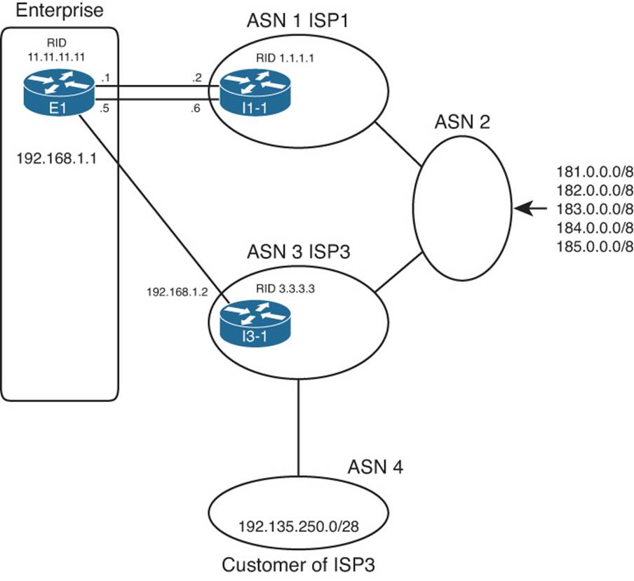
Figure 13-20 Three Prefixes to Be Advertised to E1
The show ip bgp output lists the entirety of the BGP routing table. Example 13-6 shows a sample from Router E1. Note that the configuration of this network is based on Example 13-2, with Routers E1 and I1-1 still using their loopback interfaces in their neighbor commands.
Example 13-6 E1’s BGP Table with Routes Learned from the ISPs
E1# show ip bgp
BGP table version is 78, local router ID is 11.11.11.11
Status codes: s suppressed, d damped, h history, * valid, > best, i - internal,
r RIB-failure, S Stale
Origin codes: i - IGP, e - EGP, ? - incomplete
Network Next Hop Metric LocPrf Weight Path
* 0.0.0.0 192.168.1.2 0 0 3 i
*> 1.1.1.1 0 0 1 i
*> 181.0.0.0/8 1.1.1.1 0 1 2 111 111 i
*> 182.0.0.0/8 1.1.1.1 0 1 2 222 i
*> 183.0.0.0/8 1.1.1.1 0 1 2 i
*> 184.0.0.0/8 1.1.1.1 0 1 2 i
*> 185.0.0.0/8 1.1.1.1 0 1 2 i
* 192.135.250.0/28 1.1.1.1 0 1 2 3 4 i
*> 192.168.1.2 0 3 4 i
First, examine the overall format and the headings in the output of the show ip bgp command. The Network column lists the prefix/length (NLRI). The Next Hop heading lists the next-hop IP address that would be used for the route. Then, skipping over to the far right, the Path heading lists the AS_PATH PA. (Note that it is difficult to see the beginning of the AS_PATH, but the weight [another PA] for each route is 0 in this case. So, the next number after the 0, in this case, is the beginning of the AS_PATH.)
Next, focus on the last two lines of output from the show ip bgp command. Each of the last two lines describes a different route to reach 192.135.250.0/28—one with next-hop 1.1.1.1 (Router I1-1) and one with next-hop 192.168.1.2 (Router I3-1). Because the second of these two lines does not list a prefix (under the heading “Network”), the output implies that this line is just another route for the prefix listed on the previous line. Next, examine the highlighted AS_PATH values at the end of each of these lines. For the route through I1-1 (1.1.1.1), the AS_PATH lists ASNs 1, 2, 3, and 4. Similarly, the AS_PATH for the other route lists only ASNs 3 and 4.
Note
The show ip bgp command lists the AS_PATH with the first-added ASN on the right and the last-added ASN on the left. BGP uses this convention, because when BGP adds an ASN to the AS_PATH, BGP prepends the ASN to the list, causing the new ASN to show up as the leftmost ASN in the AS_PATH.
Continuing to focus on the final two lines of the show ip bgp output, examine the far left part of the output and note that the second of these two lines has a > highlighted. Per the legend at the top of the command output, the > denotes the chosen best route. In this case, none of the routers inside the various ISPs set PAs for the purpose of influencing the best-path choice, so the first-used BGP best-path decision is the shortest AS_PATH. As a result, the path through ISP3, ASN 3, is best, having only two ASNs, compared to the path through ISP1, ASN 1, with four ASNs.
You can confirm that all of E1’s BGP table entries were learned using eBGP, rather than iBGP, by the absence of the letter “i” in the third column. Immediately after the *>, a space appears in the output. If a route were learned with iBGP, an “i” would appear in this third character position. By implication, all the routes in Example 13-6 are eBGP routes because of the absence of the letter “i” in the third character of possible output.
Finally, taking a broader view of the output of the show ip bgp command, consider which prefixes have two known routes and which have only one. Then, consider the design requirements listed before Example 13-6: I1-1 would advertise all prefixes, plus a default, but I3-1 would advertise only partial updates plus a default. As such, I3-1 did not advertise the prefixes that begin 181 through 185, by design, resulting in Router E1 only learning one route for each of these prefixes.
E1 chose the route through I3-1 as the best route for prefix 192.135.250.0/28. Example 13-7 shows the details of the IP routing table entry for this route.
Example 13-7 E1’s IP Route for 192.135.250.0/28
E1# show ip route 192.135.250.0 255.255.255.240
Routing entry for 192.135.250.0/28
Known via "bgp 11", distance 20, metric 0
Tag 3, type external
Last update from 192.168.1.2 00:10:27 ago
Routing Descriptor Blocks:
* 192.168.1.2, from 192.168.1.2, 00:10:27 ago
Route metric is 0, traffic share count is 1
AS Hops 2
Route tag 3
The output of the show ip route 192.135.250.0 255.255.255.240 command lists the source of the route (BGP process 11), the next-hop router (192.168.1.2), and the AS Path length (AS Hops 2). The output also confirms that the route is an external (eBGP) route.
Viewing Subsets of the BGP Table
When accepting full or partial BGP updates, the sheer number of BGP table entries can be much too large for the show ip bgp command to be useful. The command could list thousands, or even hundreds of thousands, of prefixes. In practice, you need to be comfortable with a variety of options on the show ip bgp command, each listing a different part of the BGP table.
For example, you will likely want to look at BGP table entries for specific prefixes, including the default route prefix of 0.0.0.0/0. Additionally, you might want to see routes per neighbor, and see which routes were heard from that neighbor—and which of those routes passed through any inbound route filters to make it into the BGP table. Finally, to verify whether neighboring ISPs sent full or partial updates, you can look at counters for the number of prefixes learned from each neighbor. Although you probably will never know the exact number of prefixes to expect, you should see a significant difference in the number of prefixes learned from a neighbor sending full updates as compared to a neighbor sending partial updates.
Table 13-8 summarizes some of the key command options that can supply these subsets of information.
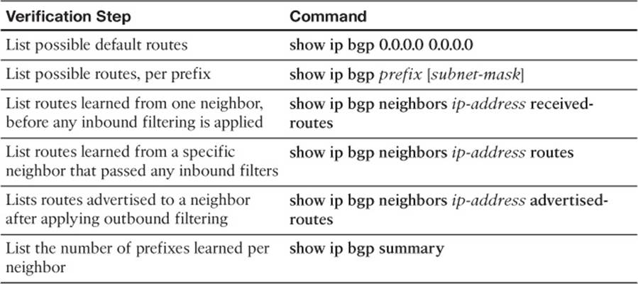
Table 13-8 Verification Commands for eBGP-Learned Routes
Example 13-8 shows a few samples of these commands on Router E1 from Figures 13-16 and 13-20.
Example 13-8 Command Samples from Table 13-8
E1# show ip bgp 0.0.0.0 0.0.0.0
BGP routing table entry for 0.0.0.0/0, version 75
Paths: (2 available, best #2, table Default-IP-Routing-Table)
Advertised to update-groups:
1
3
192.168.1.2 from 192.168.1.2 (3.3.3.3)
Origin IGP, metric 0, localpref 100, valid, external
1
1.1.1.1 from 1.1.1.1 (1.1.1.1)
Origin IGP, metric 0, localpref 100, valid, external, best
E1# show ip bgp 192.135.250.0
BGP routing table entry for 192.135.250.0/28, version 78
Paths: (2 available, best #2, table Default-IP-Routing-Table)
Advertised to update-groups:
1
1 2 3 4
1.1.1.1 from 1.1.1.1 (1.1.1.1)
Origin IGP, localpref 100, valid, external
3 4
192.168.1.2 from 192.168.1.2 (3.3.3.3)
Origin IGP, localpref 100, valid, external, best
E1# show ip bgp summary
BGP router identifier 11.11.11.11, local AS number 11
BGP table version is 78, main routing table version 78
7 network entries using 924 bytes of memory
9 path entries using 468 bytes of memory
8/5 BGP path/bestpath attribute entries using 1184 bytes of memory
7 BGP AS-PATH entries using 168 bytes of memory
0 BGP route-map cache entries using 0 bytes of memory
0 BGP filter-list cache entries using 0 bytes of memory
Bitfield cache entries: current 1 (at peak 2) using 32 bytes of memory
BGP using 2776 total bytes of memory
BGP activity 7/0 prefixes, 53/44 paths, scan interval 60 secs
Neighbor V AS MsgRcvd MsgSent TblVer InQ OutQ Up/Down State/PfxRcd
1.1.1.1 4 1 186 189 78 0 0 00:53:33 7
192.168.1.2 4 3 161 199 78 0 0 00:51:48 2
The first command, show ip bgp 0.0.0.0 0.0.0.0, displays details about the default routes in the BGP table. The output lists three lines per route, with the AS_PATH on the first line. Working through the highlighted portions of the output, in this case, the AS_PATH is either 3 or 1, because the ISP routers each originated the route, and those neighboring ASNs are ASN 1 and ASN 3. The output also lists the next-hop address of the route (192.168.1.2 and 1.1.1.1) and the neighbor’s BGP RID (I1-1’s is 1.1.1.1 and I3-1’s is 3.3.3.3). Finally, instead of the > seen in the output of show ip bgp, this command simply lists the term “best” for the best route.
The next command, show ip bgp 192.135.250.0, looks much like the first. In this case, with no subnet mask listed in the command, Cisco IOS displays information for any prefix 192.135.250.0 regardless of prefix length. The output again lists three lines per route beginning with the AS_PATH values (as highlighted).
The final command, listed earlier in Table 13-8, show ip bgp summary, lists the number of prefixes received from each neighbor on the far right side. Also, you can see the amount of memory used for the prefixes (listed as network entries) and for different PAs.
The rest of the commands from Table 13-8 focus on displaying information relative to whether BGP filtering has yet occurred. The first, show ip bgp neighbors ip-address received-routes, lists routes received from the neighbor before inbound BGP filtering. The second, show ip bgp neighbors ip-address routes, lists routes received from that neighbor that passed through any inbound filtering. These commands are particularly useful when verifying the results of any configured BGP filters or route maps.
Injecting Routes into BGP for Advertisement to the ISPs
So far, this chapter has focused on configuring eBGP peers and the routes learned by enterprise routers from eBGP peers at ISPs. These outbound routes let the enterprise routers forward packets toward the Internet.
At the same time, the ISPs need to learn routes for the enterprise’s public IP address space. This chapter assumes that the choice to use BGP has already been made, so using BGP to advertise the enterprise’s public IP address range makes good sense. This short final major section of this chapter examines the options for advertising these routes. Specifically, this section looks at two options:
![]() BGP network command
BGP network command
![]() Redistribution from an IGP
Redistribution from an IGP
Injecting Routes Using the network Command
The BGP network router subcommand differs significantly from the network command used by IGPs. For OSPF and EIGRP, the network command lists parameters that the router then compares to all its interface IP addresses. If matched, the router enables the IGP routing protocol on those interfaces. BGP does not use the network command to enable BGP on interfaces—in fact, BGP has no concept of being enabled on interfaces. For a point of comparison, note that the show ip ospf interface and show ip eigrp interfaces commands identify the enabled interfaces for OSPF and EIGRP, respectively, but no such equivalent BGP command even exists.
The BGP network command does cause a comparison to occur, but the comparison occurs between the network command’s parameters and the contents of that router’s IP routing table, as follows:
Look for a route in the router’s current IP routing table that exactly matches the parameters of the network command; if a route for that exact prefix/length exists, put the equivalent prefix/length into the local BGP table.
Note
The preceding statement, and the remaining logic in this section, assumes a BGP default setting of no auto-summary. The effect of reversing this setting to auto-summary is described in the next section.
For example, the enterprise shown earlier on the left side of Figure 13-16 might use a private address range and use NAT to translate to usable public addresses. For example, the enterprise might use private Class A network 10.0.0.0 for all private address needs and public address block 128.107.0.0/19 for public addresses. Enterprise Router E1 would then need to advertise the public prefix (128.107.0.0/19) to its ISPs, but not the private address range. Example 13-9 shows an example.
Example 13-9 E1’s Configuration of a network Command to Advertise Prefixes with eBGP
router bgp 11
network 128.107.0.0 mask 255.255.224.0
E1# sh ip bgp
BGP table version is 9, local router ID is 11.11.11.11
Status codes: s suppressed, d damped, h history, * valid, > best, i - internal,
r RIB-failure, S Stale
Origin codes: i - IGP, e - EGP, ? - incomplete
Network Next Hop Metric LocPrf Weight Path
* 0.0.0.0 192.168.1.2 0 0 3 i
*> 1.1.1.1 0 0 1 i
*> 128.107.0.0/19 10.1.1.66 3 32768 i
*> 181.0.0.0/8 1.1.1.1 0 1 2 111 111 i
*> 182.0.0.0/8 1.1.1.1 0 1 2 222 i
*> 183.0.0.0/8 1.1.1.1 0 1 2 i
*> 184.0.0.0/8 1.1.1.1 0 1 2 i
*> 185.0.0.0/8 1.1.1.1 0 1 2 i
* 192.135.250.0/28 1.1.1.1 0 1 2 3 4 i
*> 192.168.1.2 0 3 4 i
The network 128.107.0.0 mask 255.255.224.0 command lists both the subnet number and mask. It adds this prefix to the BGP table only if the exact prefix with that same mask exists in Router E1’s routing table. In this case, such a route existed, so the show ip bgp command output that follows now lists 128.107.0.0/19 in the BGP table.
In some cases, the Internet-connected router might not have a single route for the entire public prefix. For example, with such a large range of public addresses as 128.107.0.0/19, the enterprise will most likely have broken that range into subnets, and the enterprise router might not have a route for the entire range. For example, Router E1 might see routes for 128.107.1.0/24, 128.107.2.0/24, and so on but no route for 128.107.0.0/19.
When a router knows routes only for subsets of the prefix that needs to be advertised, an additional step is needed when using the network command. For example, the network 128.107.0.0 mask 255.255.224.0 command will not add this prefix to the BGP table even if routes for subsets of this range exist, such as 128.107.1.0/24. So, either configure a static route for the entire range, with outgoing interface null0, on the Internet-facing router, or use IGP route summarization to create a summary route for the entire prefix with IGP.
Note
The static route for 128.107.0.0/19 to null0—a discard route—is not meant to be advertised to other routers. Its only purpose is to enable the operation of the network command. This discard route should not cause routing problems on the local router, because of the more specific routes for subnets inside the same range of addresses.
Finally, the network command examples in this section use the mask parameter, but if omitted, Cisco IOS assumes a classful network mask. For example, a network 9.0.0.0 command assumes a Class A default mask of 255.0.0.0, and the network 128.1.0.0 command assumes a Class B default mask of 255.255.0.0.
The Effect of auto-summary on the BGP network Command
As of Cisco IOS Release 15.1 mainline, BGP defaults to a setting of no auto-summary, and the previous section’s discussion of the network command assumed this default setting. However, if the configuration is changed to auto-summary, Cisco IOS makes a small change in how it interprets the network command.
The change in logic occurs only when the network command omits its mask parameter; there is no difference in logic if the mask parameter is explicitly configured. When the network command refers to a Class A, B, or C network, with no mask parameter configured and with auto-summary configured, the router adds a route for that classful network to the BGP table under one of the following conditions:
![]() If the exact classful route is in the IP routing table
If the exact classful route is in the IP routing table
![]() If any subset routes of that classful network are in the routing table
If any subset routes of that classful network are in the routing table
In summary, of the two actions in the list, the first occurs regardless of the auto-summary setting and the second occurs only if auto-summary is configured.
For example, with network 9.0.0.0 configured, regardless of the auto-summary setting, if a route to 9.0.0.0/8 exists, the router adds 9.0.0.0/8 to the BGP table. However, if the network 9.0.0.0 (without the mask parameter) and the auto-summary commands were both configured, and if only a subset route exists (for example, 9.1.1.0/24), but no route for exactly 9.0.0.0/8 exists, the router still adds a route for the classful network (9.0.0.0/8) to the BGP table. This second example demonstrates the additional logic that occurs with the auto-summary command configured.
Injecting Routes Using Redistribution
Instead of using a BGP network command to add routes to the BGP table, the enterprise BGP routers can instead redistribute routes from an IGP into BGP. The end goals are the same:
![]() Inject the public address range, but not the private IP address range, into the BGP table.
Inject the public address range, but not the private IP address range, into the BGP table.
![]() Advertise one route for the public address range, instead of any individual subnets of the range.
Advertise one route for the public address range, instead of any individual subnets of the range.
The enterprise routers that run BGP often already run the IGP as well and have learned routes for either the entire public range as one route or with subset routes. If a single route exists for the entire public range, for example, the 128.107.0.0/19 range used in the last several examples, the engineer simply needs to add a redistribute command to the BGP configuration to redistribute that route, and only that route, into BGP. If only subset routes exist, one of several additional steps needs to be taken to meet the design goal to inject one route for the entire public address range.
Example 13-10 shows the majority of the work in a case for which Router E1 has three subset routes in the 128.107.0.0/19 range: 128.107.1.0/24, 128.107.2.0/24, and 128.107.3.0/24. However, E1 does not have a single route for the entire 128.107.0.0/19 public prefix. The configuration matches prefixes in the public range and redistributes them into BGP.
Example 13-10 Redistributing OSPF into BGP, but for Public Range Only
router bgp 11
redistribute ospf 1 route-map only-128-107
!
route-map only-128-107 permit
match ip address prefix 128-107
!
ip prefix-list 128-107 permit 128.107.0.0/19 le 32
E1# show ip route 128.107.0.0 255.255.224.0 longer-prefixes
! Legend omitted for brevity
Gateway of last resort is 1.1.1.1 to network 0.0.0.0
128.107.0.0/24 is subnetted, 3 subnets
O 128.107.3.0 [110/3] via 10.1.1.66, 00:05:26, FastEthernet0/0
O 128.107.2.0 [110/3] via 10.1.1.66, 00:05:26, FastEthernet0/0
O 128.107.1.0 [110/3] via 10.1.1.66, 00:05:36, FastEthernet0/0
E1# show ip bgp 128.107.0.0/19 longer-prefixes
BGP table version is 11, local router ID is 11.11.11.11
Status codes: s suppressed, d damped, h history, * valid, > best, i - internal,
r RIB-failure, S Stale
Origin codes: i - IGP, e - EGP, ? - incomplete
Network Next Hop Metric LocPrf Weight Path
*> 128.107.1.0/24 10.1.1.66 3 32768 ?
*> 128.107.2.0/24 10.1.1.66 3 32768 ?
*> 128.107.3.0/24 10.1.1.66 3 32768 ?
The two show commands following the configuration list the IP routes that should match the redistribution configuration, and the resulting BGP table entries. The show ip route 128.107.0.0 255.255.224.0 longer-prefixes command lists all three IP routes in the public address range in this case. The show ip bgp 128.107.0.0/19 longer-prefixes command shows the same range, listing the three BGP table entries created by the redistribute ospf command. These BGP table entries list the same next-hop IP addresses listed in the OSPF routes in the IP routing table, with the same metrics.
Left as is, this configuration results in Router E1 advertising all three BGP routes to the ISPs. However, to reach the goal of advertising only a single route for the entire public prefix 128.107.0.0/19, another step must be taken, typically one of the following:
![]() Use IGP route summarization to create the route for the entire prefix.
Use IGP route summarization to create the route for the entire prefix.
![]() Configure a null static route (a discard route) for the entire prefix on the Internet-connected router.
Configure a null static route (a discard route) for the entire prefix on the Internet-connected router.
![]() Configure BGP route summarization to make BGP advertise only the entire prefix.
Configure BGP route summarization to make BGP advertise only the entire prefix.
The first two would cause Router E1 to list a route for the entire public prefix—128.107.0.0/19 in this case—in its IP routing table. The redistribution configuration could then be changed so that only that exact prefix would be redistributed. (For example, removing the le 32 parameter from the ip prefix-list 128-107 permit 128.107.0.0/19 le 32 command would make this command match only the exact route.)
The third option would be to use BGP route summarization, telling Router E1 that when any subset routes of 128.107.0.0/19 exist in the BGP table, advertise only 128.107.0.0/19 but none of the subset routes. Example 13-11 shows this last option.
Example 13-11 BGP aggregate-address Command to Advertise the Entire Public IP Address Prefix
E1# conf t
Enter configuration commands, one per line. End with CNTL/Z.
E1(config)# router bgp 11
E1(config-router)# aggregate-address 128.107.0.0 255.255.224.0 summary-only
E1(config-router)# ^Z
E1# show ip bgp 128.107.0.0/19 longer-prefixes
BGP table version is 15, local router ID is 11.11.11.11
Status codes: s suppressed, d damped, h history, * valid, > best, i - internal,
r RIB-failure, S Stale
Origin codes: i - IGP, e - EGP, ? - incomplete
Network Next Hop Metric LocPrf Weight Path
*> 128.107.0.0/19 0.0.0.0 32768 i
s> 128.107.1.0/24 10.1.1.66 3 32768 ?
s> 128.107.2.0/24 10.1.1.66 3 32768 ?
s> 128.107.3.0/24 10.1.1.66 3 32768 ?
Note that with the addition of the aggregate-address command, the BGP table now also has a route for 128.107.0.0/19, which will be advertised to E1’s neighbors at the two ISPs. Also, the summary-only keyword in the aggregate-address command tells Cisco IOS to suppress the advertisement of the subset routes, as noted by the code “s” beside the other three routes listed at the end of the example.
Exam Preparation Tasks
Planning Practice
The CCNP ROUTE exam expects test takers to review design documents, create implementation plans, and create verification plans. This section provides some exercises that can help you to take a step back from the minute details of the topics in this chapter so that you can think about the same technical topics from the planning perspective.
For each planning practice table, simply complete the table. Note that any numbers in parentheses represent the number of options listed for each item in the solutions in Appendix F, “Completed Planning Practice Tables.”
Design Review Table
Table 13-9 lists several design goals related to this chapter. If these design goals were listed in a design document, and you had to take that document and develop an implementation plan, what implementation options come to mind? You should write a general description; specific configuration commands are not required.
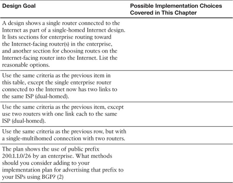
Table 13-9 Design Review
Implementation Plan Peer Review Table
Table 13-10 shows a list of questions that others might ask, or that you might think about, during a peer review of another network engineer’s implementation plan. Complete the table by answering the questions.
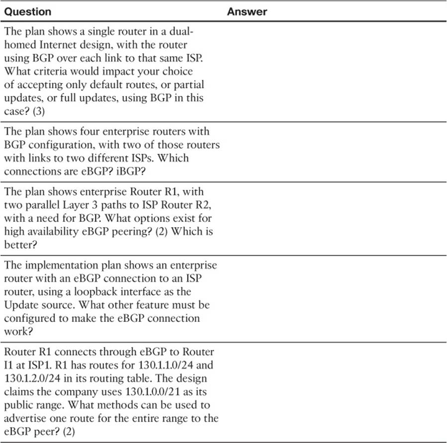
Table 13-10 Notable Questions from This Chapter to Consider During an Implementation Plan Peer Review
Create an Implementation Plan Table
This chapter does not focus on implementation or verification, but it did review one concept about static routes, as listed in Table 13-11.
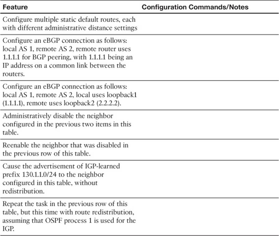
Table 13-11 Implementation Plan Configuration Memory Drill
Choose Commands for a Verification Plan Table
To practice skills useful when creating your own verification plan, list in Table 13-12 all commands that supply the requested information. You might want to record your answers outside the book and set a goal to complete this table (and others like it) from memory during your final reviews before taking the exam.
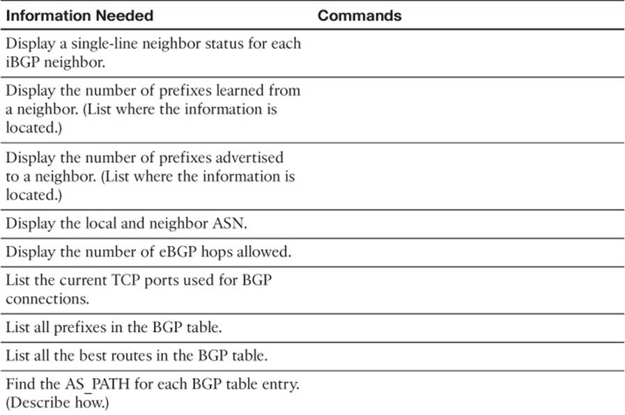
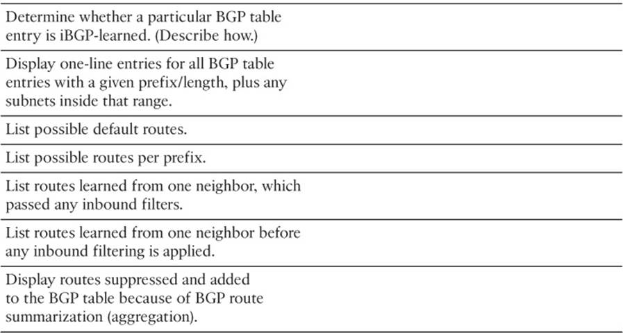
Table 13-12 Verification Plan Memory Drill
Note
Some of the entries in this table might not have been specifically mentioned in this chapter but are listed in this table for review and reference.
Review All the Key Topics
Review the most important topics from inside the chapter, noted with the Key Topic icon in the outer margin of the page. Table 13-13 lists a reference of these key topics and the page numbers on which each is found.
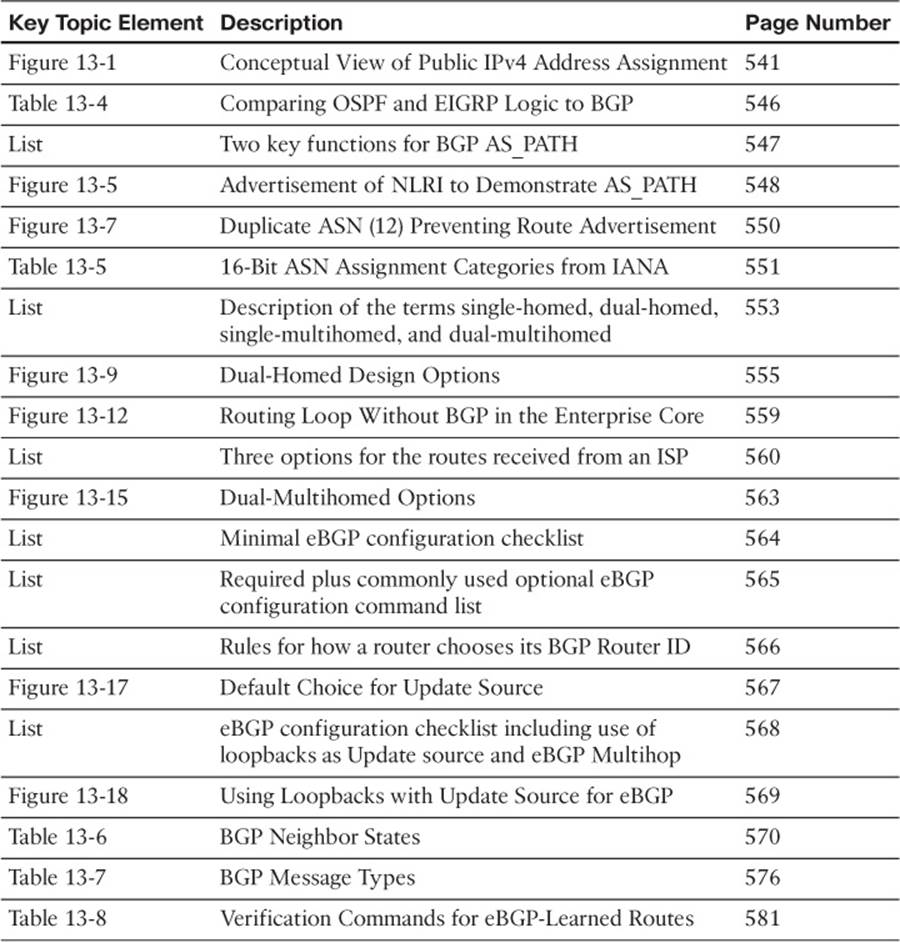
Table 13-13 Key Topics for Chapter 13
Complete the Tables and Lists from Memory
Print a copy of Appendix D, “Memory Tables,” (found on the CD) or at least the section for this chapter, and complete the tables and lists from memory. Appendix E, “Memory Tables Answer Key,” also on the CD, includes completed tables and lists to check your work.
Define Key Terms
Define the following key terms from this chapter, and check your answers in the glossary.
public IP address
private IP address
Network Address Translation (NAT)
Port Address Translation (PAT)
AS_SEQUENCE
Path Attribute (PA)
AS path
public ASN
private ASN
default route
single-homed
dual-homed
single-multihomed
dual-multihomed
autonomous system number (ASN)
eBGP multihop
Update Source (BGP)
Established (BGP state)
Open
Update
Active (BGP state)
BGP table