Advanced EIGRP Concepts - IGP Routing Protocols - CCNP Routing and Switching ROUTE 300-101 Official Cert Guide (2015)
CCNP Routing and Switching ROUTE 300-101 Official Cert Guide (2015)
Part II. IGP Routing Protocols
Chapter 5. Advanced EIGRP Concepts
This chapter covers the following subjects:
Building the EIGRP Topology Table: This section discusses how a router seeds its local EIGRP topology table, and how neighboring EIGRP routers exchange topology information.
Building the IP Routing Table: This section explains how routers use EIGRP topology data to choose the best routes to add to their local routing tables.
Optimizing EIGRP Convergence: This section examines items that have an impact on how fast EIGRP converges for a given route.
Route Filtering: This section examines how to filter prefixes from being sent in EIGRP Updates or filter them from being processed when received in an EIGRP Update.
Route Summarization: This section discusses the concepts and configuration of EIGRP route summarization.
Default Routes: This section examines the benefits of using default routes, and the mechanics of two methods for configuring default routes with EIGRP.
Enhanced Interior Gateway Routing Protocol (EIGRP), like Open Shortest Path First (OSPF), uses three major branches of logic, each of which populates a different table. EIGRP begins by forming neighbor relationships and listing those relationships in the EIGRP neighbor table (as described in Chapter 4, “Fundamental EIGRP Concepts”). EIGRP then exchanges topology information with these same neighbors, with newly learned information being added to the router’s EIGRP topology table. Finally, each router processes the EIGRP topology table to choose the best IP routes currently available, adding those IP routes to the IP routing table.
This chapter moves from the first major branch (neighborships, as covered in Chapter 4) to the second and third branches: EIGRP topology and EIGRP routes. To that end, the first major section of this chapter describes the protocol used by EIGRP to exchange the topology information and details exactly what information EIGRP puts in its messages sent between routers. The next major section shows how EIGRP examines the topology data to then choose the best route currently available for each prefix. The final section of this chapter examines how to optimize the EIGRP convergence processes so that when the topology does change, the routers in the internetwork quickly converge to the then-best routes. This chapter concludes with three sections covering categories of tools that you can use to limit the number of routes in the routing table: route filtering, route summarization, and default routes.
“Do I Know This Already?” Quiz
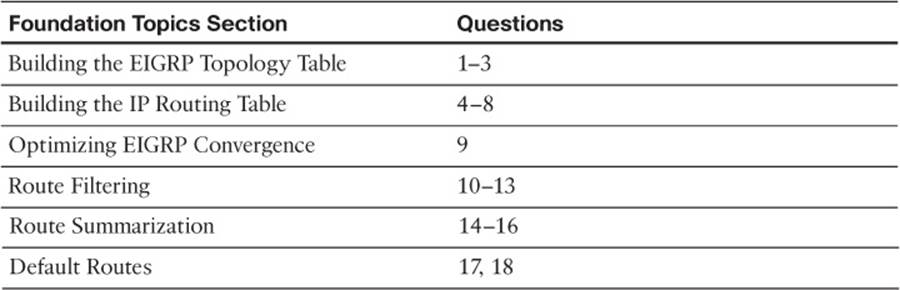
The “Do I Know This Already?” quiz allows you to assess whether you should read the entire chapter. If you miss no more than two of these 18 self-assessment questions, you might want to move ahead to the “Exam Preparation Tasks” section. Table 5-1 lists the major headings in this chapter and the “Do I Know This Already?” quiz questions covering the material in those headings, so that you can assess your knowledge of these specific areas. The answers to the “Do I Know This Already?” quiz appear in Appendix A.
Table 5-1“Do I Know This Already?” Foundation Topics Section-to-Question Mapping
1. Which of the following are methods that EIGRP uses to initially populate (seed) its EIGRP topology table, before learning topology data from neighbors? (Choose two.)
a. By adding all subnets listed by the show ip route connected command
b. By adding the subnets of working interfaces over which static neighbors have been defined
c. By adding subnets redistributed on the local router from another routing source
d. By adding all subnets listed by the show ip route static command
2. Which of the following are both advertised by EIGRP in the Update message and included in the formula for calculating the integer EIGRP metric? (Choose two.)
a. Jitter
b. Delay
c. MTU
d. Reliability
3. Router R1 uses S0/0 to connect through a T/1 to the Frame Relay service. Five PVCs terminate on the serial link. Three PVCs (101, 102, and 103) are configured on subinterface S0/0.1, and one each (104 and 105) are on S0/0.2 and S0/0.3. The configuration shows no configuration related to EIGRP WAN bandwidth control, and the bandwidth command is not configured. Which of the following is true about how Cisco IOS tries to limit EIGRP’s use of bandwidth on S0/0?
a. R1 limits EIGRP to around 250 kbps on DLCI 102.
b. R1 limits EIGRP to around 250 kbps on DLCI 104.
c. R1 limits EIGRP to around 150 kbps on every DLCI.
d. R1 does not limit EIGRP because no WAN bandwidth control has been configured.
4. The output of show ip eigrp topology on Router R1 shows the following output, which is all the output related to subnet 10.11.1.0/24. How many feasible successor routes does R1 have for 10.11.1.0/24?
P 10.11.1.0/24, 2 successors, FD is 2172419 via 10.1.1.2 (2172423/28167), Serial0/0/0.1 via 10.1.1.6 (2172423/28167), Serial0/0/0.2
a. 0
b. 1
c. 2
d. 3
5. A network design shows that R1 has four different possible paths from itself to the data center subnets. Which of the following can influence which of those routes become feasible successor routes, assuming that you follow the Cisco-recommended practice of not changing metric weights? (Choose two.)
a. The configuration of EIGRP offset lists
b. Current link loads
c. Changing interface delay settings
d. Configuration of variance
6. Router R1 is three router hops away from subnet 10.1.1.0/24. According to various show interfaces commands, all three links between R1 and 10.1.1.0/24 use the following settings: bandwidth (in kbps): 1000, 500, 100000 and delay (in microseconds): 12000, 8000, 100. Which of the following answers correctly identify a value that feeds into the EIGRP metric calculation? (Choose two.)
a. Bandwidth of 101,500 kilobits per second
b. Bandwidth of about 34,000 kilobits per second
c. Bandwidth of 500 kilobits per second
d. Delay of 1200 tens-of-microseconds
e. Delay of 2010 tens-of-microseconds
f. Delay of 20100 tens microseconds
7. Routers R1 and R2 are EIGRP neighbors. R1 has been configured with the eigrp stub connected command. Which of the following are true as a result? (Choose two.)
a. R1 can learn EIGRP routes from R2, but R2 cannot learn EIGRP routes from R1.
b. R1 can send IP packets to R2, but R2 cannot send IP packets to R1.
c. R2 no longer learns EIGRP routes from R1 for routes not connected to R1.
d. R1 no longer replies to R2’s Query messages.
e. R2 no longer sends Query messages to R1.
8. Router R1 lists four routes for subnet 10.1.1.0/24 in the output of the show ip eigrp topology all-links command. The variance 100 command is configured, but no other related commands are configured. Which of the following rules is true regarding R1’s decision of what routes to add to the IP routing table? Note that RD refers to reported distance and FD to feasible distance.
a. Adds all routes for which the metric is <= 100 * the best metric among all routes
b. Adds all routes because of the ridiculously high variance setting
c. Adds all successor and feasible successor routes
d. Adds all successor and feasible successor routes for which the metric is <= 100 * the best metric among all routes
9. A network design shows that R1 has four possible paths from itself to the data center subnets. Which of the following commands is most likely to show you all the possible next-hop IP addresses for these four possible routes?
a. show ip eigrp topology
b. show ip eigrp topology all-links
c. show ip route eigrp
d. show ip route eigrp all-links
e. show ip eigrp topology all-learned
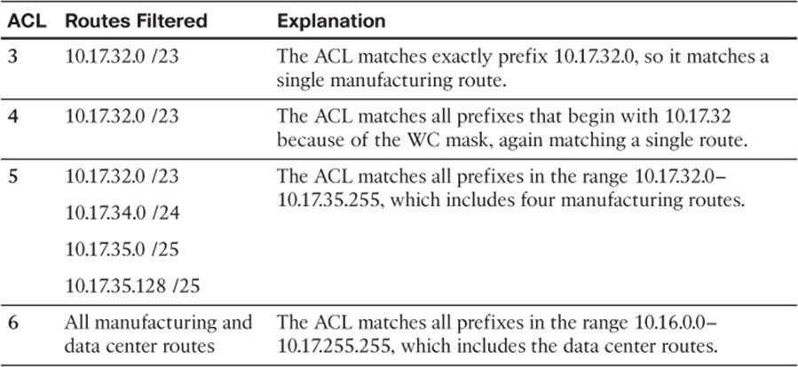
10. Router R1 has been configured for EIGRP. The configuration also includes an ACL with one line—access-list 1 permit 10.10.32.0 0.0.15.255—and the EIGRP configuration includes the distribute-list 1 in command. Which of the following routes could not be displayed in the output of the show ip eigrp topology command as a result? (Choose two.)
a. 10.10.32.0 /19
b. 10.10.44.0 /22
c. 10.10.40.96 /27
d. 10.10.48.0 /23
e. 10.10.60.0 /30
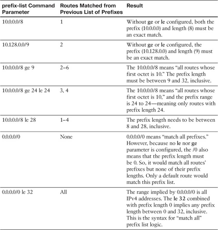
11. The command output that follows was gathered from Router R1. If correctly referenced by an EIGRP distribution list that filters outbound Updates, which of the following statements are true about the filtering of various prefixes by this prefix list? (Choose three.)
R1# sh ip prefix-list ip prefix-list question: 3 entries seq 5 deny 10.1.2.0/24 ge 25 le 27 seq 15 deny 10.2.0.0/16 ge 30 le 30 seq 20 permit 0.0.0.0/0
a. Prefix 10.1.2.0/24 will be filtered because of clause 5.
b. Prefix 10.1.2.224/26 will be filtered because of clause 5.
c. Prefix 10.2.2.4/30 will be filtered because of clause 15.
d. Prefix 10.0.0.0/8 will be permitted.
e. Prefix 0.0.0.0/0 will be permitted.
12. R1 has correctly configured EIGRP to filter routes using a route map named question. The configuration that follows shows the entire route map and related configuration. Which of the following is true regarding the filtering action on prefix 10.10.10.0/24 in this case?
route-map question deny 10 match ip address 1 route-map question permit 20 match ip address prefix-list fred ! access-list 1 deny 10.10.10.0 0.0.0.255 ip prefix-list fred permit 10.10.10.0/23 le 25
a. It will be filtered because of the deny action in route map clause 10.
b. It will be allowed because of the double negative (two deny references) in clause 10.
c. It will be permitted because of matching clause 20’s reference to prefix-list fred.
d. It will be filtered because of matching the implied deny all route map clause at the end of the route map.
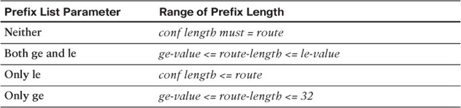
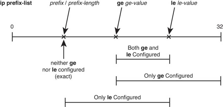
13. An engineer has typed four different single-line prefix lists in a word processor. The four answers show the four different single-line prefix lists. The engineer then does a copy/paste of the configuration into a router. Which of the lists could match a subnet whose prefix length is 27? (Choose two.)
a. ip prefix-list fred permit 10.0.0.0/24 ge 16 le 28
b. ip prefix-list barney permit 10.0.0.0/24 le 28
c. ip prefix-list wilma permit 10.0.0.0/24 ge 25
d. ip prefix-list betty permit 10.0.0.0/24 ge 28
14. An engineer plans to configure summary routes with the ip summary-address eigrpasn prefix mask command. Which of the following, when added to such a command, would create a summary that includes all four of the following subnets: 10.1.100.0/25, 10.1.101.96/27, 10.1.101.224/28, and 10.1.100.128 /25?
a. 10.1.0.0 255.255.192.0
b. 10.1.64.0 255.255.192.0
c. 10.1.100.0 255.255.255.0
d. 10.1.98.0 255.255.252.0
15. R1 has five working interfaces, with EIGRP neighbors existing off each interface. R1 has routes for subnets 10.1.1.0/24, 10.1.2.0/24, and 10.1.3.0/24, with EIGRP integer metrics of roughly 1 million, 2 million, and 3 million, respectively. An engineer then adds the ip summary-address eigrp 1 10.1.0.0 255.255.0.0 command to interface Fa0/0. Which of the following is true?
a. R1 loses and then reestablishes neighborships with all neighbors.
b. R1 no longer advertises 10.1.1.0/24 to neighbors connected to Fa0/0.
c. R1 advertises a 10.1.0.0/16 route out Fa0/0, with metric of around 3 million (largest metric of component subnets).
d. R1 advertises a 10.1.0.0/16 route out Fa0/0, with metric of around 2 million (median metric of component subnets).
16. In a lab, R1 connects to R2, which connects to R3. R1 and R2 each have several working interfaces, all assigned addresses in Class A network 10.0.0.0. Router R3 has some working interfaces in Class A network 10.0.0.0, and others in Class B network 172.16.0.0. The engineer experiments with the auto-summary command on R2 and R3, enabling and disabling the command in various combinations. Which of the following combinations will result in R1 seeing a route for 172.16.0.0 /16, instead of the individual subnets of Class B network 172.16.0.0? (Choose two.)
a. auto-summary on R2 and no auto-summary on R3
b. auto-summary on R2 and auto-summary on R3
c. no auto-summary on R2 and no auto-summary on R3
d. no auto-summary on R2 and auto-summary on R3
17. Router R1 exists in an enterprise that uses EIGRP as its routing protocol. The show ip route command output on Router R1 lists the following phrase: “Gateway of last resort is 1.1.1.1 to network 2.0.0.0.” Which of the following is most likely to have caused this output to occur on R1?
a. R1 has been configured with an ip default-network 2.0.0.0 command.
b. R1 has been configured with an ip route 0.0.0.0 0.0.0.0 1.1.1.1 command.
c. R1 has been configured with an ip route 2.0.0.0 255.0.0.0 1.1.1.1 command.
d. Another router has been configured with an ip default-network 2.0.0.0 command.
18. Enterprise Router R1 connects an enterprise to the Internet. R1 needs to create and advertise a default route into the enterprise using EIGRP. The engineer creating the implementation plan has chosen to base this default route on the ip route command, rather than using ip default-network. Which of the following are not useful steps with this style of default route configuration? (Choose two.)
a. Create the default route on R1 using the ip route 0.0.0.0 0.0.0.0 outgoing-interface command.
b. Redistribute the statically configured default route.
c. Disable auto-summary.
d. Configure the network 0.0.0.0 command.
e. Ensure that R1 has no manually configured summary routes using the ip summary-address eigrp command.
Foundation Topics
Building the EIGRP Topology Table
The overall process of building the EIGRP topology table is relatively straightforward. EIGRP defines some basic topology information about each route for each unique prefix/length (subnet). This basic information includes the prefix, prefix length, metric information, and a few other details. EIGRP neighbors exchange topology information, with each router storing the learned topology information in its respective EIGRP topology table. EIGRP on a given router can then analyze the topology table, or topology database, and choose the best route for each unique prefix/length.
EIGRP uses much simpler topology data than does OSPF, which is a link-state protocol that must describe the entire topology of a portion of a network with its topology database. EIGRP, essentially an advanced distance vector protocol, does not need to define nearly as much topology data, nor do EIGRP routers need to run the complex Shortest Path First (SPF) algorithm. This first major section examines the EIGRP topology database, how routers create and flood topology data, and some specific issues related to WAN links.
Seeding the EIGRP Topology Table
Before a router can send EIGRP topology information to a neighbor, that router must have some topology data in its topology table. Routers can, of course, learn about subnets and the associated topology data from neighboring routers. However, to get the process started, each EIGRP router needs to add topology data for some prefixes so that it can then advertise these routes to its EIGRP neighbors. A router’s EIGRP process adds subnets to its local topology table, without learning the topology data from an EIGRP neighbor, from three sources:
Prefixes of connected subnets for interfaces on which EIGRP has been enabled on that router using the network command
Prefixes of connected subnets for interfaces referenced in an EIGRP neighbor command
Prefixes learned by the redistribution of routes into EIGRP from other routing protocols or routing information sources
After a router adds such prefixes to its local EIGRP topology database, that router can then advertise the prefix information, along with other topology information associated with each prefix, to each working EIGRP neighbor. Each router adds any learned prefix information to its topology table, and then that router advertises the new information to other neighbors. Eventually, all routers in the EIGRP domain learn about all prefixes unless some other feature, such as route summarization or route filtering, alters the flow of topology information.
The Content of EIGRP Update Message
EIGRP uses five basic protocol messages to do its work:
Hello
Update
Query
Reply
ACK (acknowledgment)
EIGRP uses two messages as part of the topology data exchange process: Update and ACK. The Update message contains the topology information, whereas the ACK acknowledges receipt of the update packet.
The EIGRP Update message contains the following information:
Prefix
Prefix length
Metric components: bandwidth, delay, reliability, and load
Nonmetric items: MTU and hop count
Note
Many courses and books over the years have stated that MTU is part of the EIGRP metric. In practice, the MTU has never been part of the metric calculation, although it is included in the topology data for each prefix.
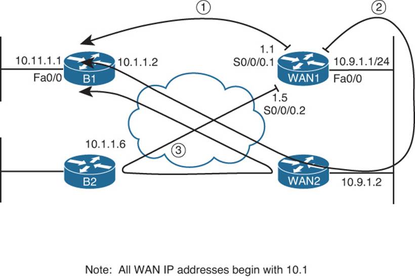
To examine this entire process in more detail, see Figure 5-1 and Figure 5-2.
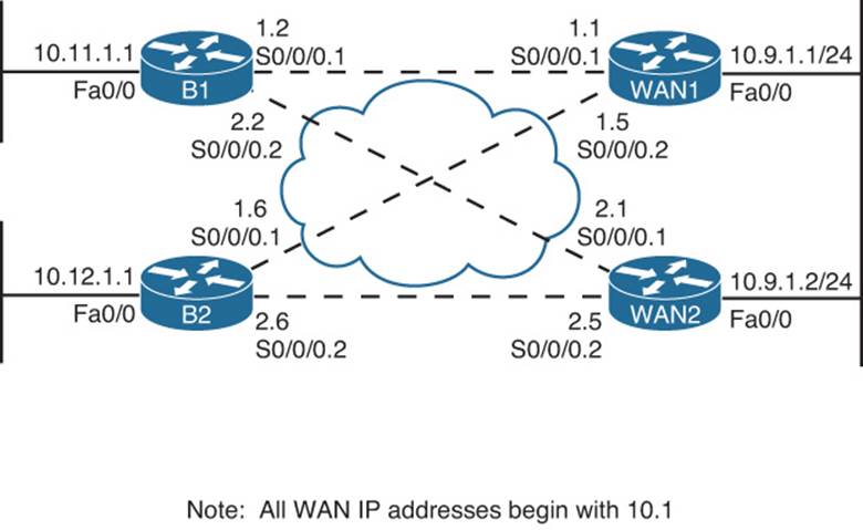
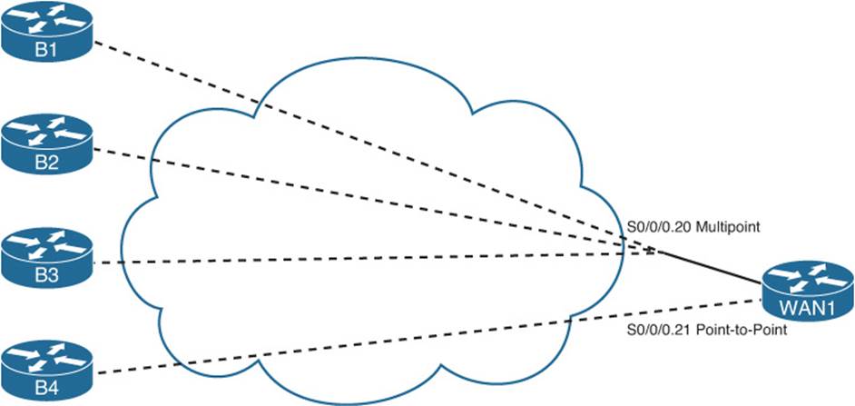
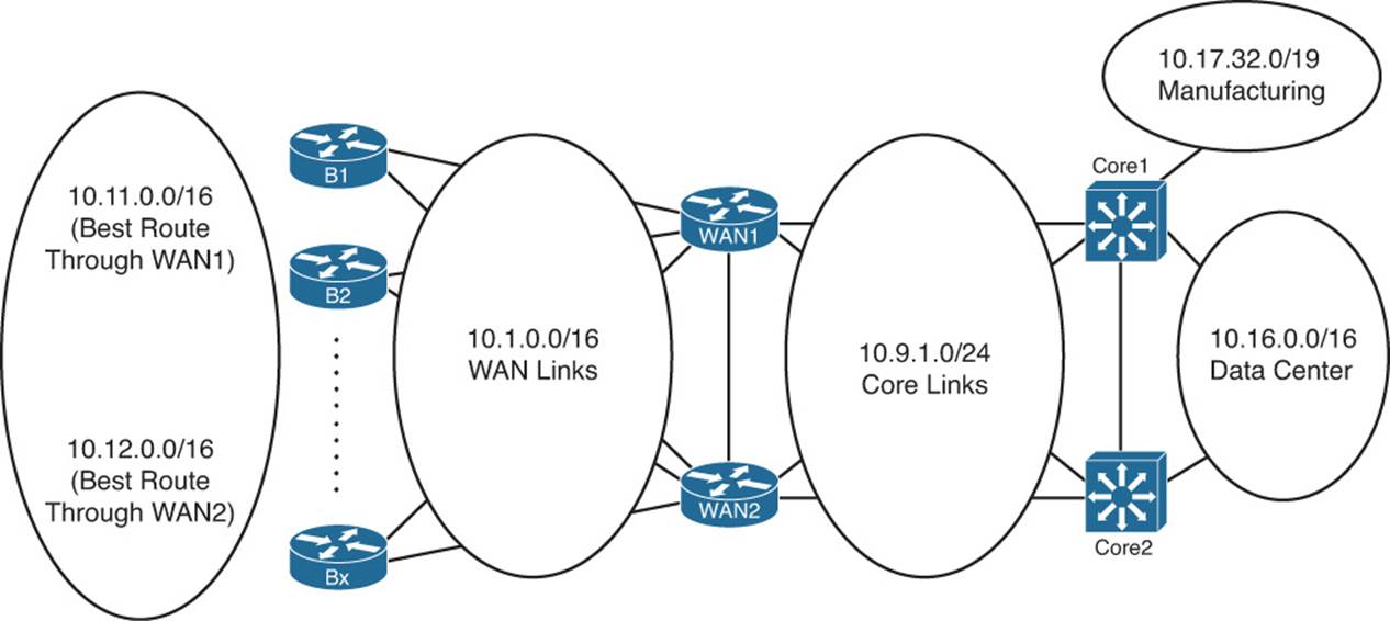
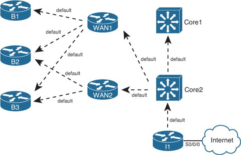
Figure 5-1Typical WAN Distribution and Branch Office Design
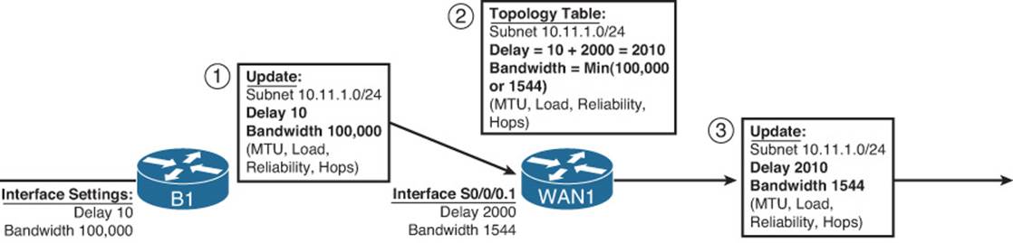
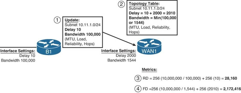
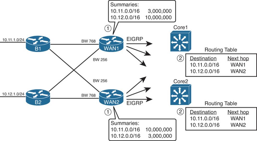
Figure 5-2Contents of EIGRP Update Messages
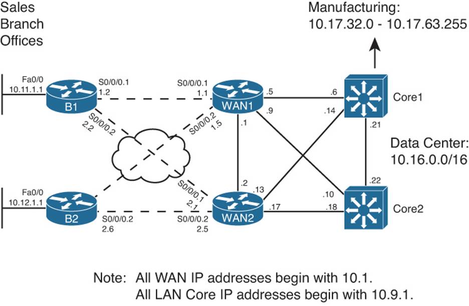
Figure 5-1 shows a portion of an enterprise network that will be used in several examples in this chapter. Routers B1 and B2 represent typical branch office routers, each with two Frame Relay permanent virtual circuits (PVC) connected back to the main site. WAN1 and WAN2 are WAN distribution routers, each of which could have dozens or hundreds of PVCs.
The routers in Figure 5-1 have been configured and work. For EIGRP, all routers have been configured with as many defaults as possible, with the only configuration related to EIGRP being the router eigrp 1 and network 10.0.0.0 commands on each router.
Next, consider what Router B1 does for its connected route for subnet 10.11.1.0/24, which is located on B1’s LAN. B1 matches its Fa0/0 interface IP address (10.11.1.1) because of its network 10.0.0.0 configuration command. So, as mentioned earlier, B1 seeds its own topology table with an entry for this prefix. This topology table entry also lists the interface bandwidth of the associated interface and delay of the associated interface. Using default settings for Fast Ethernet interfaces, B1 uses a bandwidth of 100,000 kbps (the same as 100 Mbps) and a delay of 10, meaning 10 tens-of-microseconds. Router B1 also includes a default setting for the load (1) and reliability (255), even though the router, using the default K-value settings, will not use these values in its metric calculations. Finally, B1 adds to the topology database the MTU of the local interface and a hop count of 0 because the subnet is connected.
Now that B1 has added some topology information to its EIGRP topology database, Figure 5-2 shows how B1 propagates the topology information to router WAN1 and beyond.
The steps in Figure 5-2 can be explained as follows:
Step 1. B1 advertises the prefix (10.11.1.0/24) using an EIGRP Update message. The message includes the four metric components, plus MTU and hop count—essentially the information in B1’s EIGRP topology table entry for this prefix.
Step 2. WAN1 receives the Update message and adds the topology information for 10.11.1.0/24 to its own EIGRP topology table, with these changes:
WAN1 considers the interface on which it received the Update (S0/0/0.1) to be the outgoing interface of a potential route to reach 10.11.1.0/24.
WAN1 adds the delay of S0/0/0.1 (2000 tens-of-microseconds per Figure 5-2) to the delay listed in the Update message.
WAN1 compares the bandwidth of S0/0/0.1 (1544 kbps per Figure 5-2) to the bandwidth listed in the Update message (100,000 kbps) and chooses the lower value (1544) as the bandwidth for this route.
WAN1 also updates load (highest value), reliability (lowest value), and MTU (lowest value) based on similar comparisons, and adds 1 to the hop count.
Step 3. WAN1 then sends an Update to its neighbors, with the metric components listed in their own topology table.
This example provides a good backdrop to understand how EIGRP uses cumulative delay and minimum bandwidth in its metric calculation. Note that at Step 2, Router WAN1 adds to the delay value but does not add the bandwidth. For bandwidth, WAN1 simply chooses the lowest bandwidth, comparing the bandwidth of its own interface (S0/0/0.1) with the bandwidth listed in the received EIGRP update.
Next, consider this logic on other routers (not shown in the figure) as WAN1 floods this routing information throughout the enterprise. WAN1 then sends this topology information to another neighbor, and that router sends the topology data to another, and so on. If the bandwidth of those links were 1544 or higher, the bandwidth setting used by those routers would remain the same, because each router would see that the routing update’s bandwidth (1544 kbps) was lower than the link’s bandwidth. However, each router would add something to the delay.
As a final confirmation of the contents of this Update process, Example 5-1 shows the details of the EIGRP topology database for prefix 10.11.1.0/24 on both B1 and WAN1.
Example 5-1Topology Database Contents for 10.11.1.0/24, on B1 and WAN1
! On Router B1:
The highlighted portions of the output match the details shown in Figure 5-2, but with one twist relating to the units on the delay setting. The Cisco IOS delay command, which lets you set the delay, along with the data stored in the EIGRP topology database, uses a unit of tens-of-microseconds. However, the show interfaces and show ip eigrp topology commands list delay in a unit of microseconds. For example, WAN1’s listing of “20100 microseconds” matches the “2010 tens-of-microseconds” shown in Figure 5-2.
The EIGRP Update Process
So far, this chapter has focused on the detailed information that EIGRP exchanges with a neighbor about each prefix. This section takes a broader look at the process.
When EIGRP neighbors first become neighbors, they begin exchanging topology information using Update messages using these rules:
When a neighbor first comes up, the routers exchange full updates, meaning that the routers exchange all topology information.
After all prefixes have been exchanged with a neighbor, the updates cease with that neighbor if no changes occur in the network. There is no subsequent periodic reflooding of topology data.
If something changes—for example, one of the metric components changes, links fail, links recover, or new neighbors advertise additional topology information—the routers send partial updates about only the prefixes whose status or metric components have changed.
If neighbors fail and then recover, or new neighbor adjacencies are formed, full updates occur over these adjacencies.
EIGRP uses Split Horizon rules on most interfaces by default, which impacts exactly which topology data EIGRP sends during both full and partial updates.
Split Horizon, the last item in the list, needs a little more explanation. Split Horizon limits the prefixes that EIGRP advertises out an interface. Specifically, if the currently best route for a prefix lists a particular outgoing interface, Split Horizon causes EIGRP to not include that prefix in the Update sent out that same interface. For example, router WAN1 uses S0/0/0.1 as its outgoing interface for subnet 10.11.1.0/24. So, WAN1 would not advertise prefix 10.11.1.0/24 in its Update messages sent out S0/0/0.1.
To send the Updates, EIGRP uses the Reliable Transport Protocol (RTP) to send the EIGRP Updates and confirm their receipt. On point-to-point topologies such as serial links, MPLS VPNs, and Frame Relay networks when using point-to-point subinterfaces, the EIGRP Update and ACK messages use a simple process of acknowledging each Update with an ACK. On multiaccess data links, EIGRP typically sends Update messages to multicast address 224.0.0.10 and expects a unicast EIGRP ACK message from each neighbor in reply. RTP manages that process, setting timers so that the sender of an Update waits a reasonable time, but not too long, before deciding whether all neighbors received the Update or whether one or more neighbors did not reply with an ACK.
Interestingly, although EIGRP relies on the RTP process, network engineers cannot manipulate how this works.
WAN Issues for EIGRP Topology Exchange
With all default settings, after you enable EIGRP on all the interfaces in an internetwork, the topology exchange process typically does not pose any problems. However, a few scenarios exist, particularly on Frame Relay, which can cause problems. This section summarizes two issues and shows the solutions.
Split Horizon Default on Frame Relay Multipoint Subinterfaces
Cisco IOS support for Frame Relay allows the configuration of IP addresses on the physical serial interface, multipoint subinterfaces, or point-to-point subinterfaces. Additionally, IP packets can be forwarded over a PVC even when the routers on the opposite ends do not have to use the same interface or subinterface type. As a result, many small intricacies exist in the operation of IP and IP routing protocols over Frame Relay, particularly related to default settings on different interface types.
Frame Relay supports several reasonable configuration options using different interfaces and subinterfaces, each meeting different design goals. For example, if a design includes a few centralized WAN distribution routers, with PVCs connecting each branch router to each distribution router, both distribution and branch routers might use point-to-point subinterfaces. Such a choice makes the Layer 3 topology simple, with all links acting like point-to-point links from a Layer 3 perspective. This choice also removes issues such as Split Horizon.
In some cases, a design might include a small set of routers that have a full mesh of PVCs connecting each. In this case, multipoint subinterfaces might be used, consuming a single subnet and reducing the consumption of the IP address space. This choice also reduces the number of subinterfaces.
Both options—using point-to-point subinterfaces or using multipoint subinterfaces—have legitimate reasons for being used. However, when using the multipoint subinterface option, a particular EIGRP issue can occur when the following are true:
Three or more routers, connected over a Frame Relay network, are configured as part of a single subnet.
The routers use multipoint interfaces.
Either permanently or for a time, a full mesh of PVCs between the routers does not exist.
For example, consider Router WAN1 shown earlier in Figure 5-1 and referenced again in Figure 5-3. In the earlier configurations, the WAN distribution routers and branch routers all used point-to-point subinterfaces and a single subnet per VC. To see the problem raised in this section, consider that same internetwork, but now the engineer has chosen to configure WAN1 to use a multipoint subinterface and a single subnet for WAN1, B1, and B2, as shown in Figure 5-3.
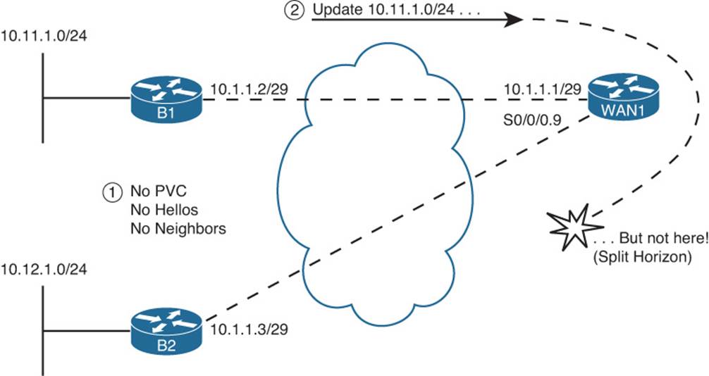
Figure 5-3Partial Mesh, Central Sites (WAN1) Uses Multipoint Subinterface
The first issue to consider in this design is that B1 and B2 will not become EIGRP neighbors with each other, as noted with Step 1 in the figure. EIGRP routers must be reachable using Layer 2 frames before they can exchange EIGRP Hello messages and become EIGRP neighbors. In this case, there is no PVC between B1 and B2. B1 exchanges Hellos with WAN1, and they become neighbors, as will B2 with WAN1. However, routers do not forward received EIGRP Hellos, so WAN1 will not receive a Hello from B1 and forward it to B2 or vice versa. In short, although in the same subnet (10.1.1.0/29), B1 and B2 will not become EIGRP neighbors.
The second problem occurs because of Split Horizon logic on Router WAN1, as noted with Step 2 in the figure. As shown with Step 2, B1 could advertise its routes to WAN1, and WAN1 could advertise those routes to B2—and vice versa. However, with default settings, WAN1 will not advertise those routes because of its default setting of Split Horizon (a default interface subcommand setting of ip split-horizon eigrpasn). As a result, WAN1 receives the Update from B1 on its S0/0/0.9 subinterface, but Split Horizon prevents WAN1 from advertising that topology data to B2 in Updates sent out interface S0/0/0.9, and vice versa.
The solution is somewhat simple—just configure the no ip split-horizon eigrpasn command on the multipoint subinterface on WAN1. The remote routers, B1 and B2 in this case, still do not become neighbors, but that does not cause a problem by itself. With Split Horizon disabled on WAN1, B1 and B2 learn routes to the other branch’s subnets. Example 5-2 lists the complete configuration and the command to disable Split Horizon. Also shown in Example 5-2 is the output of the show ip eigrp interfaces detail s0/0/0.9 command, which shows the operational state of Split Horizon on that subinterface.
Note
Frame Relay configuration is considered a prerequisite, because it is part of the CCNA exam and courses. Example 5-2 uses frame-relay interface-dlci commands and relies on Inverse ARP. However, if frame-relay map commands were used instead, disabling Inverse ARP, the EIGRP details discussed in this example would remain unchanged.
Example 5-2Frame Relay Multipoint Configuration on WAN1
! On Router WAN1:
Note
The [no] ip split-horizon command controls Split Horizon behavior for RIP; the [no] ip split-horizon eigrpasn command controls Split Horizon behavior for EIGRP.
EIGRP WAN Bandwidth Control
In a multiaccess WAN, one physical link passes traffic for multiple data link layer destinations. For example, a WAN distribution router connected to many branches using Frame Relay might literally terminate hundreds, or even thousands, of Frame Relay PVCs.
In a nonbroadcast multiaccess (NBMA) medium such as Frame Relay, when a router needs to send EIGRP updates, the Updates cannot be multicasted at Layer 2. So, the router must send a copy of the Update to each reachable neighbor. For a WAN distribution router with many Frame Relay PVCs, the sheer amount of traffic sent over the Frame Relay access link might overload the link.
The EIGRP WAN bandwidth control allows the engineer to protect a multiaccess Frame Relay interface from being overrun with too much EIGRP message traffic. By default, a router sends EIGRP messages out an interface but only up to 50 percent of the bandwidth defined on the interface with the bandwidth command. The engineer can adjust this percentage using the ip bandwidth-percent eigrpasn percent interface/subinterface subcommand. Regardless of the percentage, Cisco IOS then limits the rate of sending the EIGRP messages so that the rate is not exceeded. To accomplish this, Cisco IOS queues the EIGRP messages in memory, delaying them briefly.
The command to set the bandwidth percentage is simple, but there are a few caveats to keep in mind when trying to limit the bandwidth consumed by EIGRP:
The Cisco IOS default for bandwidth on serial interfaces and subinterfaces is 1544 (kbps).
EIGRP limits the consumed bandwidth based on the percentage of interface/subinterface bandwidth.
This feature keys on the bandwidth of the interface or subinterface through which the neighbor is reachable, so don’t set only the physical interface bandwidth and forget the subinterfaces.
Recommendation: Set the bandwidth of point-to-point links to the speed of the Committed Information Rate (CIR) of the single PVC on the subinterface.
General recommendation: Set the bandwidth of multipoint subinterfaces to around the total CIR for all VCs assigned to the subinterface.
Note that for multipoint subinterfaces, Cisco IOS WAN bandwidth control first divides the subinterface bandwidth by the number of configured PVCs and then determines the EIGRP percentage based on that number.
For example, consider Figure 5-4, which shows a router with one multipoint subinterface and one point-to-point subinterface.
Figure 5-4WAN1, One Multipoint, One Point-to-Point
With the configuration shown in Example 5-3, WAN1 uses the following bandwidth, at most, with each neighbor:
B1, B2, and B3: 20 kbps (20% of 300 kbps / 3 VCs)
B4: 30 kbps (30% of 100 kbps)
Example 5-3Configuration of WAN1, One Multipoint, One Point-to-Point
! On Router WAN1:
Building the IP Routing Table
An EIGRP router builds IP routing table entries by processing the data in the topology table. Unlike OSPF, which uses a computationally complex SPF process, EIGRP uses a computationally simple process to determine which, if any, routes to add to the IP routing table for each unique prefix/length. This part of the chapter examines how EIGRP chooses the best route for each prefix/length and then examines several optional tools that can influence the choice of routes to add to the IP routing table.
Calculating the Metrics: Feasible Distance and Reported Distance
The EIGRP topology table entry, for a single prefix/length, lists one or more possible routes. Each possible route lists the various component metric values—bandwidth, delay, and so on. Additionally, for connected subnets, the database entry lists an outgoing interface. For routes not connected to the local router, in addition to an outgoing interface, the database entry also lists the IP address of the EIGRP neighbor that advertised the route.
EIGRP routers calculate an integer metric based on the metric components. Interestingly, an EIGRP router does this calculation both from its own perspective and from the perspective of the next-hop router of the route. The two calculated values are as follows:
Feasible Distance (FD): Integer metric for the route, from the local router’s perspective, used by the local router to choose the best route for that prefix.
Reported Distance (RD): Integer metric for the route, from the neighboring router’s perspective (the neighbor that told the local router about the route). Used by the local router when converging to a new route.
Note
Some texts use the term Advertised Distance (AD) instead of Reported Distance (RD) as used in this book. Be ready for either term on the CCNP ROUTE exam. However, this book uses RD exclusively.
Routers use the FD to determine the best route, based on the lowest metric, and use the RD when falling back to an alternative route when the best route fails (EIGRP’s use of the RD is explained in the upcoming section “Successor and Feasible Successor Concepts”). Focusing on the FD, when a router has calculated the integer FD for each possible route to reach a single prefix/length, that router can then consider adding the lowest-metric route to the IP routing table.
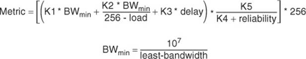
As a reminder, the following formula shows how EIGRP calculates the metric, assuming default settings of the EIGRP metric weights (K-values). The metric calculation grows when the slowest bandwidth in the end-to-end route decreases (the slower the bandwidth, the worse the metric), and its metric grows (gets worse) when the cumulative delay grows. Also, note that the unit of measure for slowest-bandwidth is kbps, and the unit of measure for cumulative-delay is tens-of-microseconds.
An example certainly helps in this case. Figure 5-5 repeats some information about the topology exchange process between Routers B1 and WAN1 (refer to Figure 5-1), essentially showing the metric components as sent by B1 to WAN1 (Step 1) and the metric components from WAN1’s perspective (Step 2).
Figure 5-5Example Calculation of RD and FD on Router WAN1
Steps 3 and 4 in Figure 5-5 show WAN1’s calculation of the RD and FD for 10.11.1.0/24, respectively. Router WAN1 takes the metric components as received from B1, and plugs them into the formula, to calculate the RD, which is the same integer metric that Router B1 would have calculated as its FD. Step 4 shows the same formula but with the metric components as listed at Step 2—after the adjustments made on WAN1. Step 4 shows WAN1’s FD calculation, which is much larger because of the much lower constraining bandwidth plus the much larger cumulative delay.
WAN1 chooses its best route to reach 10.11.1.0/24 based on the lowest FD among all possible routes. Looking back to the much more detailed Figure 5-1, presumably a couple of other routes might have been possible, but WAN1 happens to choose the route shown in Figure 5-5 as its best route. As a result, WAN1’s show ip route command lists the FD calculated in Figure 5-5 as the metric for this route, as shown in Example 5-4.
Example 5-4Router WAN1’s EIGRP Topology and IP Route Information for 10.11.1.0/24
! Below, note that WAN1's EIGRP topology table lists two possible next-hop ! routers: 10.1.1.2 (B1) and 10.9.1.2 (WAN2). The metric for each route, ! the first number in parentheses, shows that the lower metric route is the one ! through 10.1.1.2 as next-hop. Also note that the metric components ! match Figure 5-5. ! WAN1# show ip eigrp topo 10.11.1.0/24 IP-EIGRP (AS 1): Topology entry for 10.11.1.0/24 State is Passive, Query origin flag is 1, 1 Successor(s), FD is 2172416 Routing Descriptor Blocks: 10.1.1.2 (Serial0/0/0.1), from 10.1.1.2, Send flag is 0x0 Composite metric is (2172416/28160), Route is Internal Vector metric: Minimum bandwidth is 1544 Kbit Total delay is 20100 microseconds Reliability is 255/255 Load is 1/255 Minimum MTU is 1500 Hop count is 1 10.9.1.2 (FastEthernet0/0), from 10.9.1.2, Send flag is 0x0 Composite metric is (2174976/2172416), Route is Internal Vector metric: Minimum bandwidth is 1544 Kbit Total delay is 20200 microseconds Reliability is 255/255 Load is 1/255 Minimum MTU is 1500 Hop count is 2 ! ! The next command not only lists the IP routing table entry for 10.11.1.0/24, ! it also lists the metric (FD), and components of the metric. ! WAN1# show ip route 10.11.1.0 Routing entry for 10.11.1.0/24 Known via "eigrp 1", distance 90, metric 2172416, type internal Redistributing via eigrp 1 Last update from 10.1.1.2 on Serial0/0/0.1, 00:02:42 ago Routing Descriptor Blocks: * 10.1.1.2, from 10.1.1.2, 00:02:42 ago, via Serial0/0/0.1 Route metric is 2172416, traffic share count is 1 Total delay is 20100 microseconds, minimum bandwidth is 1544 Kbit Reliability 255/255, minimum MTU 1500 bytes Loading 1/255, Hops 1 ! ! Below, the route for 10.11.1.0/24 is again listed, with the metric (FD), and ! the same next-hop and outgoing interface information. ! WAN1# show ip route eigrp 10.0.0.0/8 is variably subnetted, 7 subnets, 2 masks D 10.11.1.0/24 [90/2172416] via 10.1.1.2, 00:10:40, Serial0/0/0.1 D 10.12.1.0/24 [90/2172416] via 10.1.1.6, 00:10:40, Serial0/0/0.2 D 10.1.2.0/30 [90/2172416] via 10.9.1.2, 00:10:40, FastEthernet0/0 D 10.1.2.4/30 [90/2172416] via 10.9.1.2, 00:10:40, FastEthernet0/0
EIGRP Metric Tuning
EIGRP metrics can be changed using several methods: setting interface bandwidth, setting interface delay, changing the metric calculation formula by configuring K-values, and even by adding to the calculated metric using offset lists. In practice, the most reasonable and commonly used methods are to set the interface delay and the interface bandwidth. This section examines all the methods, in part so that you will know which useful tools exist and in part to make you aware of some other design issues that then might impact the routes chosen by EIGRP.
Configuring Bandwidth and Delay
The bandwidth and delay interface subcommands set the bandwidth and delay associated with the interface. The commands themselves require little thought, other than keeping the units straight. The unit for the bandwidth command is kilobits/second, and the delay command uses a unit of tens-of-microseconds.
If a design requires that you influence the choice of route by changing bandwidth or delay, setting the delay value is typically the better choice. Cisco IOS uses the bandwidth setting of an interface for many other reasons: calculating interface utilization, as the basis for several QoS parameters, and for Simple Network Management Protocol (SNMP) statistics reporting. However, the delay setting has little influence on other Cisco IOS features besides EIGRP, so the better choice when influencing EIGRP metrics is to tune the delay.
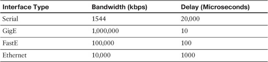
Table 5-2 lists some of the common default values for both bandwidth and delay. As a reminder, show commands list the bandwidth in kbps, which matches the bandwidth command, but lists the delay in microseconds, which does not match the tens-of-microseconds unit of the delaycommand.
Table 5-2Common Defaults for Bandwidth and Delay
Note that on LAN interfaces that can run at different speeds, the bandwidth and delay settings default based on the current actual speed of the interface.
Choosing Bandwidth Settings on WAN Subinterfaces
Frame Relay and Metro Ethernet installations often use an access link with a particular physical sending rate (clock rate if you will) but with the contracted speed, over time, being more or less than the speed of the link. For example, with Frame Relay, the provider might supply a full T1 access link, so configuring bandwidth 1544 for such an interface is reasonable. However, the subinterfaces have one or more PVCs associated with them, and those PVCs each have Committed Information Rates (CIR) that are typically less than the access link’s clock speed. However, the cumulative CIRs for all PVCs often exceed the clock rate of a physical interface. Conversely, MetroE designs use Ethernet access links of 10-Mbps, 100-Mbps, or 1-Gbps actual link speed, but often the business contract limits the amount of traffic to some number below that link speed.
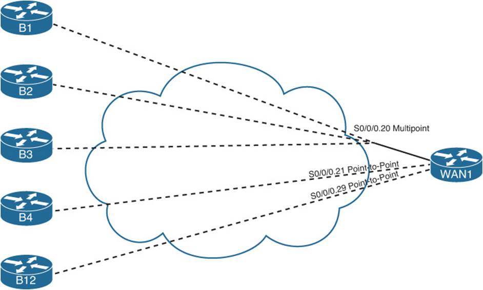
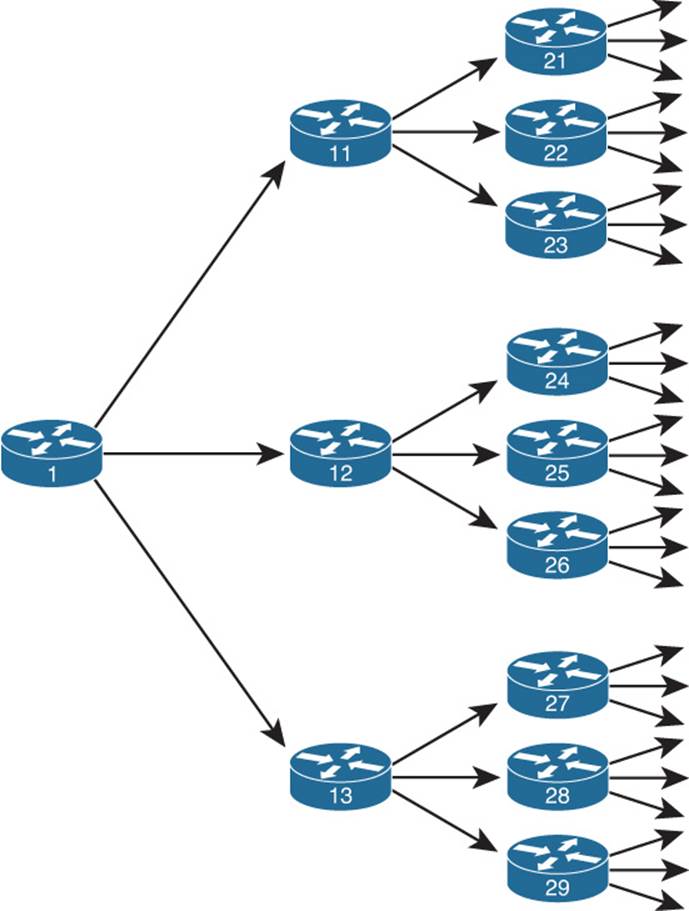
Choosing a useful interface bandwidth setting on the subinterfaces in a Frame Relay or MetroE design requires some thought, with most of the motivations for choosing one number or another being unrelated to EIGRP. For example, imagine the network shown in Figure 5-6. Router WAN1 has a single T1 (1.544-Mbps) access link. That interface has one multipoint subinterface, with three PVCs assigned to it. It also has nine other point-to-point subinterfaces, each with a single PVC assigned.
Figure 5-6One Multipoint and Nine Point-to-Point Subinterfaces
For the sake of discussion, the design in Figure 5-6 oversubscribes the T1 access link off Router WAN1 by a 2:1 factor. Assume that all 12 PVCs have a CIR of 256 kbps, making the total bandwidth for the 12 PVCs roughly 3 Mbps. The design choice to oversubscribe the access link might be reasonable given the statistical chance of all sites sending at the same time.
Now imagine that Router WAN1 has been configured with subinterfaces as shown in the figure:
S0/0/0.20: Multipoint, 3 PVCs
S0/0/0.21 through S0/0/0.29: Point-to-point, 1 PVC each
Next, consider the options for setting the bandwidth command’s value on these ten subinterfaces. The point-to-point subinterfaces could be set to match the CIR of each PVC (256 kbps, in this example). You could choose to set the bandwidth based on the CIR of all combined PVCs on the multipoint subinterface—in this case, setting bandwidth 768 on multipoint subinterface s0/0/0.20. However, these bandwidths would total about 3 Mbps—twice the actual speed of WAN1’s access link. Alternatively, you could set the various bandwidths so that the total matches the 1.5 Mbps of the access link. Or you could split the difference, knowing that during times of low activity to most sites, that the sites with active traffic get more than their CIR’s worth of capacity anyway.
As mentioned earlier, these bandwidth settings impact much more than EIGRP. The settings impact interface statistics, both in show commands and in SNMP reporting. They impact QoS features to some extent as well. Given that the better option for setting EIGRP metrics is to set the interface delay, EIGRP metric tuning might not be the driving force behind the decision as to what bandwidth values to use. However, some installations might change these values over time while trying to find the right compromise numbers for features other than EIGRP. So, you need to be aware that changing those values might result in different EIGRP metrics and impact the choices of best routes.
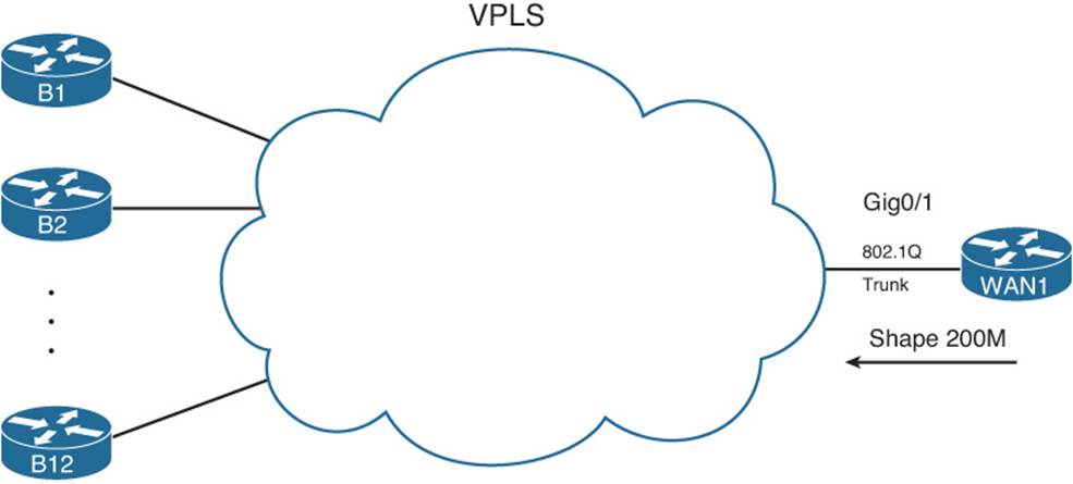
Similar issues exist on the more modern Layer 2 WAN services like MetroE, particularly with the multipoint design of Virtual Private LAN Service (VPLS). Figure 5-7 shows a design that might exist after migrating the internetwork of Figure 5-6 to VPLS. Router WAN1 has been replaced by a Layer 3 switch, using a Gigabit interface to connect to the VPLS service. The remote sites might use the same routers as before, using a Fast Ethernet interface, and might be replaced with Layer 3 switch hardware as well.
Figure 5-7VPLS Service—Issues in Choosing Bandwidth
Concentrating on the mechanics of what happens at the central site, WAN1 might use 802.1Q trunking. With 12 remote sites, WAN1 configures 12 VLAN interfaces, one per VLAN, with a different subnet used for the connection to each remote branch. Such a design, from a Layer 3 perspective, looks like the age-old Frame Relay design with a point-to-point link from the main site to each remote branch.
Additionally, the VPLS business contract might specify that WAN1 cannot send more than 200 Mbps of traffic into the VPLS cloud, with the excess being discarded by the VPLS service. To prevent unnecessary discards, the engineer likely configures a feature called shaping, which reduces the average rate of traffic leaving the Gi0/1 interface of WAN1 (regardless of VLAN). To meet the goal of 200 Mbps, WAN1 would send only part of the time—in this case averaging a sending rate of 1/5th of the time—so that the average rate is 1/5th of 1 Gbps, or 200 Mbps.
Of note with the shaping function, the shaping feature typically limits the cumulative traffic on the interface, not per VLAN (branch). As a result, if the only traffic waiting to be sent by WAN1 happens to be destined for branch B1, WAN1 sends 200 Mbps of traffic to just branch B1.
Pulling the discussion back around to EIGRP, as with Frame Relay, other design and implementation needs can drive the decision to set or change the bandwidth on the associated interfaces. In this case, Layer 3 switch WAN1 probably has 12 VLAN interfaces. Each VLAN interface can be set with a bandwidth that influences EIGRP route choices. Should this setting be 1/12th of 1 Gbps, what is the speed at which the bits are actually sent? Should the setting be 1/12th of 200 Mbps, what is the shaping rate? Or knowing that a site might get most or all of that 200 Mbps for some short period of time, should the bandwidth be set somewhere in between? As with Frame Relay, there is no set answer. For the sake of EIGRP, be aware that changes to the bandwidth settings impact the EIGRP metrics.
Metric Weights (K-values)
Engineers can change the EIGRP metric calculation by configuring the weightings (also called K-values) applied to the EIGRP metric calculation. To configure new values, use the metric weightstos k1 k2 k3 k4 k5 command in EIGRP configuration mode. To configure this command, configure any integer 0–255 inclusive for the five K-values. By default, K1 = K3 = 1, and the others default to 0. The tos parameter has only one valid value, 0, and can be otherwise ignored.
The full EIGRP metric formula is as follows. Note that some items reduce to 0 if the corresponding K-values are also set to 0.
With default K-values, the EIGRP metric calculation can be simplified to the following formula:
EIGRP requires that two routers’ K-values match before those routers can become neighbors. Also note that Cisco recommends against using K-values K2, K4, and K5, because a nonzero value for these parameters causes the metric calculation to include interface load and reliability. The load and reliability change over time, which causes EIGRP to reflood topology data, and might cause routers to repeatedly choose different routes (route flapping).
Offset Lists
EIGRP offset lists, the final tool for manipulating the EIGRP metrics listed in this chapter, allow an engineer to simply add a value—an offset, if you will—to the calculated integer metric for a given prefix. To do so, an engineer can create and enable an EIGRP offset list that defines the value to add to the metric, plus some rules regarding which routes should be matched and therefore have the value added to their computed FD.
An offset list can perform the following functions:
Match prefixes/prefix lengths using an IP ACL, so that the offset is applied only to routes matched by the ACL with a permit clause.
Match the direction of the Update message, either sent (out) or received (in).
Match the interface on which the Update is sent or received.
Set the integer metric added to the calculation for both the FD and RD calculations for the route.
The configuration itself uses the following command in EIGRP configuration mode, in addition to any referenced IP ACLs:
For example, consider again branch office Router B1 in Figure 5-1, with its connection to both WAN1 and WAN2 over a Frame Relay network. Formerly, WAN1 calculated a metric of 2,172,416 for its route, through B1, to subnet 10.11.1.0/24. (Refer to Figure 5-5 for the math behind WAN1’s calculation of its route to 10.11.1.0/24.) Router B1 also calculated a value of 28,160 for the RD of that same direct route. Example 5-5 shows the addition of an offset on WAN1, for received updates from Router B1.
Example 5-5Inbound Offset of 3 on WAN1, for Updates Received on S0/0/0.1
WAN1(config)# access-list 11 permit10.11.1.0 WAN1(config)# router eigrp 1 WAN1(config-router)# offset-list 11 in 3 Serial0/0/0.1 WAN1(config-router)# end
Mar 2 11:34:36.667: %DUAL-5-NBRCHANGE: IP-EIGRP(0) 1: Neighbor 10.1.1.2 (Serial0/0/0.1) is resync: peer graceful-restart WAN1# show ip eigrp topo 10.11.1.0/24 IP-EIGRP (AS 1): Topology entry for 10.11.1.0/24 State is Passive, Query origin flag is 1, 1 Successor(s), FD is 2172416 Routing Descriptor Blocks: 10.1.1.2 (Serial0/0/0.1), from 10.1.1.2, Send flag is 0x0 Composite metric is (2172419/28163), Route is Internal Vector metric: Minimum bandwidth is 1544 Kbit Total delay is 20100 microseconds Reliability is 255/255 Load is 1/255 Minimum MTU is 1500 Hop count is 1 ! output omitted for brevity
The configuration has two key elements: ACL 11 and the offset-list command. ACL 11 matches prefix 10.11.1.0, and that prefix only, with a permit clause. The offset-list 11 in 3 s0/0/0.1 command tells Router WAN1 to examine all EIGRP Updates received on S0/0/0.1, and if prefix 10.11.1.0 is found, add 3 to the computed FD and RD for that prefix.
The show ip eigrp topology 10.11.1.0/24 command in Example 5-5 shows that the FD and RD, highlighted in parentheses, are now each three larger as compared with the earlier metrics.
Next, continuing this same example, Router B1 has now been configured to add an offset (4) in its sent updates to all routers, but for prefix 10.11.1.0/24 only, as demonstrated in Example 5-6.
Example 5-6Outbound Offset of 4 on B1, for Updates Sent to All Neighbors, 10.11.1.0/24
B1(config)# access-list 12 permit10.11.1.0 B1(config)# router eigrp 1 B1(config-router)# offset-list 12 out 4 B1(config-router)# end B1#
! Back to router WAN1 WAN1# show ip eigrp topology IP-EIGRP Topology Table for AS(1)/ID(10.9.1.1)
Codes: P - Passive, A - Active, U - Update, Q - Query, R - Reply, r - reply Status, s - sia Status
P 10.11.1.0/24, 1 successors, FD is 2172419 via 10.1.1.2 (2172423/28167), Serial0/0/0.1 ! lines omitted for brevity
Note that the metrics, both FD and RD, are now four larger than in Example 5-5.
Unequal Metric Route Load Sharing
Convergence to a feasible successor route should happen within a second after a router realizes the successor route has failed. Even in large well-designed networks, particularly with features like stub routers and route summarization in use, convergence can still happen in a reasonable amount of time even when going active. The next feature, load sharing, takes convergence to another level, giving instantaneous convergence, while reaching other goals as well.
Cisco IOS allows routing protocols to place multiple routes into the routing table for an individual prefix/length. Cisco IOS then balances traffic across those routes, by default balancing traffic on a per-destination IP address basis.
Load balancing, sometimes called load sharing, provides a primary benefit of making use of the available bandwidth, rather than using some links as simply backup links. For example, with the two-PVC design shown previously in Figure 5-1, without load sharing, a branch router would send traffic over one PVC, but not both. With load sharing, some traffic would flow over each PVC.
A useful secondary benefit—faster convergence—occurs when using load balancing. By placing multiple routes into the routing table for a single prefix, convergence happens essentially instantly. For example, if a branch router has two routes for each data center subnet—one using each PVC that connects the branch to the core—and one of the routes fails, the other route is already in the routing table. In this case, the router does not need to look for FS routes nor go active on the route. The router uses the usual EIGRP convergence tools only when all such routes are removed from the routing table.
The load-balancing configuration requires two commands, one of which already defaults to a reasonable setting. First, you need to define the number of allowed routes for each prefix/prefix length using the maximum-pathsnumber EIGRP subcommand. The default setting of 4 is often high enough, because most internetworks do not have enough redundancy to have more than four possible routes.
Note
The maximum number of paths varies based on Cisco IOS version and router platform. However, for the much older Cisco IOS versions, the maximum was 6 routes, with later versions typically supporting 16 or more.
The second part of the load-balancing configuration overcomes a challenge introduced by EIGRP’s metric calculation. The EIGRP integer metric calculation often results in 8- to 10-digit integer metrics, so the metrics of competing routes are seldom the exact same value. Calculating the exact same metric for different routes for the same prefix is statistically unlikely.
Cisco IOS includes the concept of EIGRP variance to overcome this problem. Variance lets you tell Cisco IOS that the EIGRP metrics can be close in value and still be considered worthy of being added to the routing table—and you can define how close.
The variancemultiplier EIGRP router subcommand defines an integer in the range of 1 through 128. The router then multiplies the variance by the successor route’s FD—the metric of the best route to reach that subnet. Any FS routes whose metric is less than or equal to the product of the variance by the FD are considered to be equal routes and can be placed into the routing table, up to and including the number of routes defined by the maximum-paths command.
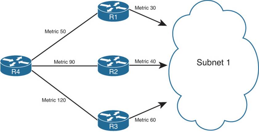
For example, consider the example as shown in Figure 5-8 and Table 5-3. In this example, to keep the focus on the concepts, the metrics are small easy-to-compare numbers, rather than the usual large EIGRP metrics. The example focuses on R4’s three possible routes to reach Subnet 1. The figure shows the RD of each route next to Routers R1, R2, and R3, respectively.
Figure 5-8Example of the Use of Variance
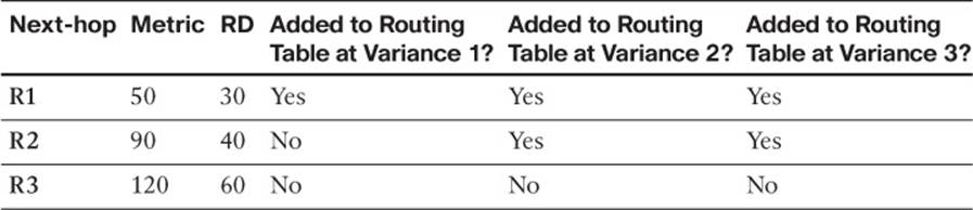
Table 5-3Example of Routes Chosen as Equal Because of Variance
Before considering the variance, note that in this case the route through R1 is the successor route, because it has the lowest metric. This also means that the FD is 50. The route through R2 is an FS route, because its RD of 40 is less than the FD of 50. The route through R3 is not an FS route, because R3’s RD of 60 is more than the FD of 50.
At a default variance setting of 1, the metrics must be exactly equal to be considered equal, so only the successor route is added to the routing table (the route through R1). With variance 2, the FD (50) is multiplied by the variance (2) for a product of 100. The route through R2, with FD 90, is less than 100, so R4 will add the route through R2 to the routing table as well. The router can then load-balance traffic across these two routes.
In the third case, with variance 3, the product of the FD (50) times 3 equals 150. All three routes’ calculated metrics (their FD values) are less than 150. However, the route through R3 is not an FS route, so it cannot be added to the routing table for fear of causing a routing loop. So, R4 adds only the routes through R1 and R2 to its IP routing table. (Note that the variance and maximum-paths settings can be verified by using the show ip protocols command.)
The following list summarizes the key points to know about variance:
The variance is multiplied by the current FD (the metric of the best route to reach a subnet).
Any FS routes whose calculated metric is less than or equal to the product of variance and FD are added to the IP routing table, assuming that the maximum-paths setting allows more routes.
Routes that are neither successor nor feasible successor routes can never be added to the IP routing table, regardless of the variance setting.
When the routes have been added to the routing table, the router supports a couple of methods for how to load-balance traffic across the routes. The router can load-balance the traffic proportionally with the metrics, meaning that lower metric routes send more packets. Alternately, the router can send all traffic over the lowest-metric route, with the other routes just being in the routing table for faster convergence in case the best route fails.
Optimizing EIGRP Convergence
The previous major section of this chapter focused on how EIGRP calculates metrics and how to change that metric calculation. However, that section discussed only one motivation for changing the metric: to make a router pick one route instead of another. This section, which focuses on optimizing the EIGRP convergence process, discusses another reason for choosing to manipulate the EIGRP metric calculations: faster convergence.
EIGRP converges very quickly, but EIGRP does not achieve the most optimal fast convergence times in all conditions. One design goal might be to tune EIGRP configuration settings so that EIGRP uses faster convergence methods for as many routes as possible, and when not possible, that EIGRP converge as quickly as it can without introducing routing loops. As a result, routers might converge in some cases in a second instead of tens of seconds (from the point of a router realizing that a route has failed).
For those of you who have not thought about EIGRP convergence before now, you must first get a comfortable understanding of the concept of EIGRP feasible successors—the first topic in this section. Following that, the text examines the EIGRP query process and route summarization. This section ends with EIGRP load balancing, which allows both spreading the load across multiple routes in addition to improving EIGRP convergence.
Fast Convergence to Feasible Successors
Earlier in this chapter, in the section “Calculating the Metrics: Feasible Distance and Reported Distance,” the text explains how a router, for each possible route, calculates two metric values. One value is the feasible distance (FD), which is the metric from that router’s perspective. The other metric is the reported distance (RD), which is the integer metric from the perspective of a next-hop router.
EIGRP routers use the RD value when determining whether a possible route can be considered to be a loop-free backup route called a feasible successor. This section explains the concepts and shows how to confirm the existence or nonexistence of such routes.
Successor and Feasible Successor Concepts
For each prefix/prefix length, when multiple possible routes exist, the router chooses the route with the smallest integer metric (smallest FD). EIGRP defines each such route as the successor route for that prefix, and EIGRP defines the next-hop router in such a route as the successor. EIGRP then creates an IP route for this prefix, with the successor as the next-hop router, and places that route into the IP routing table.
If more than one possible route exists for a given prefix/prefix length, the router examines these other (nonsuccessor) routes and asks this question: Can any of these routes be used immediately if the currently best route fails, without causing a routing loop? EIGRP runs a simple algorithm to identify which routes could be used without causing a routing loop, and EIGRP keeps these loop-free backup routes in its topology table. Then, if the successor route (the best route) fails, EIGRP immediately uses the best of these alternate loop-free routes for that prefix.
EIGRP calls these alternative, immediately usable, loop-free routes feasible successor routes, because they can feasibly be used as a new successor route when the current successor route fails. The next-hop router of such a route is called the feasible successor.
Note
In general conversation, the term successor might refer to the route or specifically to the next-hop router. Likewise, the term feasible successor might refer to the route, or the next-hop router, of an alternative route.
A router determines whether a route is a feasible successor based on the feasibility condition, defined as follows:
If a nonsuccessor route’s RD is less than the FD, the route is a feasible successor route.
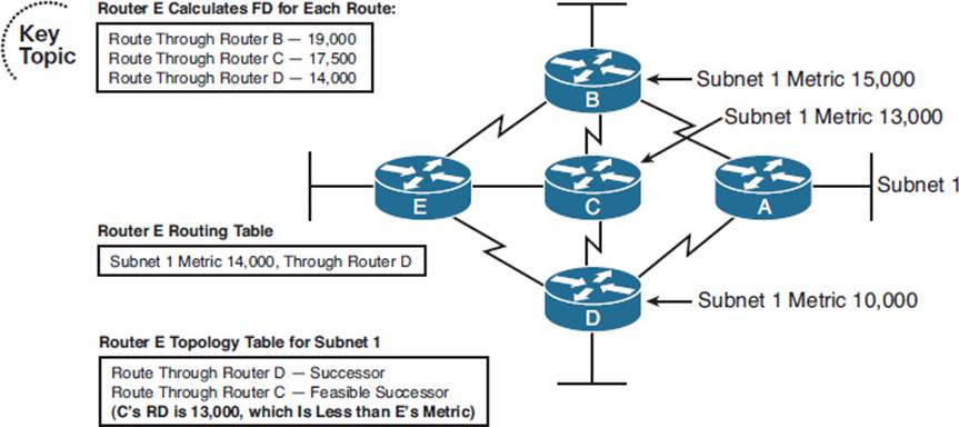
Although technically correct, the preceding definition is much more understandable with an example as shown in Figure 5-9. The figure illustrates how EIGRP figures out which routes are feasible successors for Subnet 1.
Figure 5-9Successors and Feasible Successors with EIGRP
In Figure 5-9, Router E learns three routes to Subnet 1, from Routers B, C, and D. After calculating each route’s metric, Router E finds that the route through Router D has the lowest metric. Router E adds this successor route for Subnet 1 to its routing table, as shown. The FD in this case for this successor route is 14,000.
EIGRP decides whether a route can be a feasible successor by determining whether the reported distance for that route (the metric as calculated on that neighbor) is less than its own best computed metric (the FD). If that neighbor has a lower metric for its route to the subnet in question, that route is said to have met the feasibility condition.
For example, Router E computes a metric (FD) of 14,000 on its successor route (through Router D). Router C’s computed metric—E’s RD for this alternate router through Router C—is 13,000, which is lower than E’s FD (14,000). As a result, E knows that C’s best route for this subnet could not possibly point toward Router E, so Router E believes that its route, to Subnet 1 through Router C, would not cause a loop. As a result, Router E marks its topology table entry for the route through Router C as a feasible successor route.
Conversely, E’s RD for the route through Router B to Subnet 1 is 15,000, which is larger than Router E’s FD of 14,000. So, this alternative route does not meet the feasibility condition, so Router E does not consider the route through Router B a feasible successor route.
If the route to Subnet 1 through Router D fails, Router E can immediately put the route through Router C into the routing table without fear of creating a loop. Convergence occurs almost instantly in this case. However, if both C and D fail, E would not have a feasible successor route, and would have to do additional work, as described later in the section “Converging by Going Active,” before using the route through Router B.
By tuning EIGRP metrics, an engineer can create feasible successor routes in cases where none existed, improving convergence.
Verification of Feasible Successors
Determining which prefixes have both successor and feasible successor routes is somewhat simple if you keep the following in mind:
The show ip eigrp topology command does not list all known EIGRP routes, but instead lists only successor and feasible successor routes.
The show ip eigrp topology all-links command lists all possible routes, including those that are neither successor nor feasible successor routes.
For example, consider Figure 5-10, which again focuses on Router WAN1’s route to Router B1’s LAN subnet, 10.11.1.0/24. The configuration on all routers has reverted back to defaults for all settings that impact the metric: default bandwidth and delay, no offset lists, and all interfaces are up.
Figure 5-10Three Possible Routes from WAN1 to 10.11.1.0/24
Figure 5-10 shows the three topologically possible routes to reach 10.11.1.0/24, labeled 1, 2, and 3. Route 1, direct to Router B1, is the current successor. Route 3, which goes to another branch router, back to the main site, and then to Router B1, is probably a route you would not want to use anyway. However, route 2, through WAN2, would be a reasonable backup route.
If the PVC between WAN1 and B1 failed, WAN1 would converge to route 2 from the figure. However, with all default settings, route 2 is not an FS route, as demonstrated in Example 5-7.
Example 5-7Only a Successor Route on WAN1 for 10.11.1.0/24
WAN1# show ip eigrp topology IP-EIGRP Topology Table for AS(1)/ID(10.9.1.1)
Codes: P - Passive, A - Active, U - Update, Q - Query, R - Reply, r - reply Status, s - sia Status
P 10.11.1.0/24, 1 successors, FD is 2172416 via 10.1.1.2 (2172416/28160), Serial0/0/0.1 ! lines omitted for brevity; no other lines of output pertain to 10.11.1.0/24.
WAN1# show ip eigrp topologyall-links IP-EIGRP Topology Table for AS(1)/ID(10.9.1.1)
Codes: P - Passive, A - Active, U - Update, Q - Query, R - Reply, r - reply Status, s - sia Status
P 10.11.1.0/24, 1 successors, FD is 2172416, serno 45 via 10.1.1.2 (2172416/28160), Serial0/0/0.1 via 10.9.1.2 (2174976/2172416), FastEthernet0/0 ! lines omitted for brevity; no other lines of output pertain to 10.11.1.0/24.
A quick comparison of the two commands shows that the show ip eigrp topology command shows only one next-hop address (10.1.1.2), whereas the show ip eigrp topology all-links command shows two (10.1.1.2 and 10.9.1.2). The first command lists only successor and feasible successor routes. So in this case, only one such route for 10.11.1.0/24 exists—the successor route, direct to B1 (10.1.1.2).
The output of the show ip eigrp topology all-links command is particularly interesting in this case. It lists two possible next-hop routers: 10.1.1.2 (B1) and 10.9.1.2 (WAN2). It does not list the route through Router B2 (10.1.1.6), because B2’s current successor route for 10.11.1.0/24 is through WAN1. EIGRP’s Split Horizon rules tell B2 to not advertise 10.11.1.0/24 to WAN1.
Next, focus on the route labeled as option 2 in Figure 5-9, the route from WAN1, to WAN2, then to B1. Per the show ip eigrp topology all-links command, this route has an RD of 2,172,416—the second number in parentheses as highlighted toward the end of Example 5-7. WAN1’s successor route has an FD of that exact same value. So, this one possible alternate route for 10.11.1.0/24, through WAN2, does not meet the feasibility condition—but just barely. To be an FS route, a route’s RD must be less than the FD, and in this example, the two are equal.
To meet the design requirement for quickest convergence, you could use any method to manipulate the metrics such that either WAN2’s metric for 10.11.1.0 is lower or WAN1’s metric for its successor route is higher. Example 5-8 shows the results of simply adding back the offset list on WAN1, as seen in Example 5-5, which increases WAN1’s metric by 3.
Example 5-8Increasing WAN1’s Metric for 10.11.1.0/24, Creating an FS Route
WAN1# configure terminal Enter configuration commands, one per line. End with CNTL/Z. WAN1(config)# access-list 11 permit 10.11.1.0 WAN1(config)# router eigrp 1 WAN1(config-router)# offset-list 11 in 3 s0/0/0.1 WAN1(config-router)# ^Z WAN1# show ip eigrp topology IP-EIGRP Topology Table for AS(1)/ID(10.9.1.1)
Codes: P - Passive, A - Active, U - Update, Q - Query, R - Reply, r - reply Status, s - sia Status
P 10.11.1.0/24, 1 successors, FD is 2172419 via 10.1.1.2 (2172419/28163), Serial0/0/0.1 via 10.9.1.2 (2174976/2172416), FastEthernet0/0 ! lines omitted for brevity; no other lines of output pertain to 10.11.1.0/24.
Note that now WAN1’s successor route FD is 2,172,419, which is higher than WAN2’s (10.9.1.2’s) RD of 2,172,416. As a result, WAN1’s route through WAN2 (10.9.1.2) now meets the feasibility condition. Also, the show ip eigrp topology command, which lists only successor and feasible successor routes, now lists this new feasible successor route. Also note that the output still states “1 successor.” So, this counter only counts successor routes and does not include FS routes.
When EIGRP on a router notices that a successor route has been lost, if a feasible successor exists in the EIGRP topology database, EIGRP places that feasible successor route into the routing table. The elapsed time from noticing that the route failed, until the route is replaced, is typically less than 1 second. (A Cisco Live conference presentation asserts that this convergence approaches 200 milliseconds.) With well-tuned EIGRP Hold Timers and with feasible successor routes, convergence time can be held low.
Converging by Going Active
When EIGRP removes a successor route and no FS route exists, the router begins a process by which the router discovers whether any loop-free alternative routes exist to reach that prefix. This process is called going active on a route. Routes for which the router has a successor route, and no failure has yet occurred, remain in a passive state. Routes for which the successor route fails, and no feasible successor routes exist, move to an active state, as follows:
Change the state, as listed in the show ip eigrp topology command, from passive (p) to active (a).
Send EIGRP Query messages to every neighbor except the neighbor in the failed route. The Query asks a neighbor whether that neighbor has a loop-free route for the listed prefix/length.
The neighbor considers itself to have a loop-free route if that neighbor is passive for that prefix/length. If so, the neighbor 1) sends an EIGRP Reply message, telling the original router that it does indeed have a loop-free route and 2) does not forward the Query.
If the neighbor itself is active on this route, that neighbor 1) floods EIGRP Query messages to its neighbors and 2) does not immediately send an EIGRP Reply back to the original router—instead waiting on replies to its own set of Query messages.
When a router has received Reply messages from all neighbors to which it sent any Query messages, that router can then send a Reply message to any of its neighbors as necessary.
When a router has received a Reply for all its Query messages, that router can safely use the best of the routes confirmed to be loop-free.
Note
The EIGRP convergence process when going active on a route is sometimes also referenced by the name of the underlying algorithm, named Diffusing Update Algorithm (DUAL).
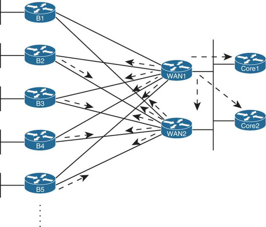
The process can and does work well in many cases, often converging to a new route in less than 10 seconds. However, in internetworks with many remote sites, with much redundancy, and with a large number of routers in a single end-to-end route, convergence when going active can be inefficient. For example, consider the internetwork in Figure 5-11. The figure shows five branch routers as an example, but the internetwork has 300 branch routers, each with a PVC connected to two WAN routers, WAN1 and WAN2. When Router WAN1 loses its route for the LAN subnet at branch B1, without an FS route, the Query process can get out of hand.
Figure 5-11Issues with Query Scope
The arrowed lines show WAN1’s Query messages and the reaction by several other routers to forward the Query messages. Although only five branch routers are shown, WAN1 would forward Query messages to 299 branch routers. WAN2 would do the same, assuming that its route to B1’s LAN also failed. These branch routers would then send Query messages back to the WAN routers. The network would converge, but more slowly than if an FS route existed.
Note
EIGRP sends every Query and Reply message using RTP, so every message is acknowledged using an EIGRP ACK message.
By configuring EIGRP so that a router has FS routes for most routes, the entire Query process can be avoided. However, in some cases, creating FS routes for all routes on all routers is impossible. So, engineers should take action to limit the scope of queries. The next two sections discuss two tools—stub routers and route summarization—that help reduce the work performed by the DUAL and the scope of Query messages.
The Impact of Stub Routers on Query Scope
Some routers, by design, should not be responsible for forwarding traffic between different sites. For example, consider the familiar internetwork shown throughout this chapter, most recently in Figure 5-11, and focus on the branch routers. If WAN2’s LAN interface failed, and WAN1’s PVC to B1 failed, a route still exists from the core to branch B1’s 10.11.1.0/24 subnet: WAN1–B2–WAN2–B1. (This is the same long route shown as route 3 in Figure 5-10.) However, this long route consumes the link bandwidth between the core and branch B2, and the traffic to/from B1 will be slower. Users at both branches will suffer, and these conditions might well be worse than just not using this long route.
Route filtering could be used to prevent WAN1 from learning such a route. However, using route filtering would require a lot of configuration on all the branch routers, with specifics for the subnets—and it would have to change over time. A better solution exists, which is to make the branch routers stub routers. EIGRP defines stub routers as follows:
A stub router is a router that should not forward traffic between two remote EIGRP-learned subnets.
To accomplish this goal, the engineer configures the stub routers using the eigrp stub command. Stub routers do not advertise EIGRP-learned routes from one neighbor to other EIGRP neighbors. Additionally, and possibly more significantly, nonstub routers note which EIGRP neighbors are stub routers, and the nonstub routers do not send Query messages to the stub routers. This action greatly reduces the scope of Query messages when a route goes active, in addition to preventing the long, circuitous, and possibly harmful route.
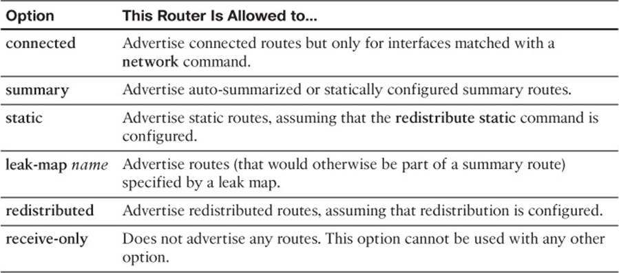
The eigrp stub command has several options. When issued simply as eigrp stub, the router uses default parameters, which are the connected and summary options. (Note that Cisco IOS adds these two parameters onto the command as added to the running config.) Table 5-4 lists the eigrp stub command options and explains some of the logic behind using them.
Table 5-4Parameters on theeigrp stubCommand
Note that stub routers still form neighborships, even in receive-only mode. The stub router simply performs less work and reduces the Query scope because neighbors will not send these routers any Query messages.
For example, Example 5-9 shows the eigrp stub connected command on Router B2, with the results being noticeable on WAN1 (show ip eigrp neighbors detail).
Example 5-9Evidence of Router B2 as an EIGRP Stub Router
B2# configure terminal B2(config)# router eigrp 1 B2(config-router)# eigrp stub connected B2(config-router)# Mar 2 21:21:52.361: %DUAL-5-NBRCHANGE: IP-EIGRP(0) 1: Neighbor 10.9.1.14 (FastEthernet0/0.12) is down: peer info changed ! A message like the above occurs for each neighbor.
! Moving to router WAN1 next WAN1# show ip eigrp neighbors detail IP-EIGRP neighbors for process 1 H Address Interface Hold Uptime SRTT RTO Q Seq (sec) (ms) Cnt Num 1 10.9.1.2 Fa0/0 11 00:00:04 7 200 0 588 Version 12.4/1.2, Retrans: 0, Retries: 0, Prefixes: 8 2 10.1.1.6 Se0/0/0.2 13 00:21:23 1 200 0 408 Version 12.4/1.2, Retrans: 2, Retries: 0, Prefixes: 2 Stub Peer Advertising ( CONNECTED ) Routes Suppressing queries 0 10.9.1.6 Fa0/0.4 12 00:21:28 1 200 0 175 Version 12.2/1.2, Retrans: 3, Retries: 0, Prefixes: 6
The Impact of Summary Routes on Query Scope
In addition to EIGRP stub routers, route summarization also limits EIGRP Query scope and therefore improves convergence time. The reduction in Query scope occurs because of the following rule:
If a router receives an EIGRP Query for a prefix/prefix length, does not have an exactly matching (both prefix and prefix length) route, but does have a summary route that includes the prefix/prefix length, that router immediately sends an EIGRP Reply and does not flood the Query to its own neighbors.
For example, consider Figure 5-12.
Figure 5-12Route Summaries Limiting Query Scope
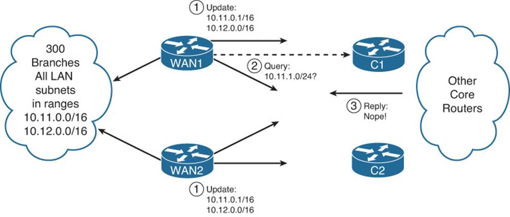
Multilayer switches C1 and C2 sit in the core of the network shown in various other figures in this chapter, and both C1 and C2 run EIGRP. The IP subnetting design assigns all branch office LAN subnets from the range 10.11.0.0/16 and 10.12.0.0/16. As such, Routers WAN1 and WAN2 advertise summary routes for these ranges, rather than for individual subnets. So, under normal operation, ignoring the entire Query scope issue, C1 and C2 would never have routes for individual branch subnets like 10.11.1.0/24 but would have routes for 10.11.0.0/16 and 10.12.0.0/16.
The figure highlights three steps:
Step 1. WAN1 and WAN2 advertise summary routes, so that C1, C2, and all other routers in the core have a route for 10.11.0.0/16 but not a route for 10.11.1.0/24.
Step 2. Some time in the future, WAN1 loses its route for 10.11.1.0/24, so WAN1 sends a Query for 10.11.1.0/24 to C1 and C2.
Step 3. C1 and C2 send an EIGRP Reply immediately afterward, because both do not have a route for that specific prefix/length (10.11.1.0/24), but both do have a summary route (10.11.0.0/16) that includes that range of addresses.
Stuck in Active
When a router notices a route failure and moves a route from the passive to active state, that router sends Query messages to its neighbors. With a sufficiently large network, particularly when routers exist several router hops away, the number of Queries might not only be large, but there also might be a string of routers that all must wait on multiple Reply messages before they can, in turn, issue a Reply. For example, in Figure 5-13, Router R1 must wait on Routers R11, R12, and R13 to send a Reply. R11 must wait on Routers R21, R22, and R23. R21 must wait on three other routers, and so on—meaning that R1 might have to wait quite a while before getting a response.
Figure 5-13Network Design That Causes Unreasonably Long Convergence
Although the design shown in Figure 5-13 is admittedly contrived, the point is that a router might wait a while before getting a Reply message in response to each Query message for an active route. A router cannot use any alternative paths for that route until all such Reply messages have been received.
To deal with this potentially long time, Cisco IOS first sets a limit on how long it should take to receive all such replies. That timer, called the active timer, is set to 3 minutes by default. (The timer can be configured for an entire EIGRP process using the timers active-timetime EIGRP subcommand, where time is represented in minutes.) Routes for which a router does not receive a Reply within the active timer are considered to be Stuck-in-Active (SIA) routes.
Cisco IOS has two major branches of logic when reacting to SIA routes. Earlier versions of Cisco IOS took a rather drastic action, bringing down the uncooperative neighbors that had yet to send back an EIGRP Reply for that route. For example, in Figure 5-12, if R1 received Reply messages from R11 and R12, but not R13, and the active timer expired, R1 would bring down the neighborship with R13. The active route would be considered to have failed, and all routes known through the failed neighbor would also be considered to have failed—possibly generating more Query messages for other routes.
Later Cisco IOS versions (beginning in the 12.2 mainline) make an attempt to avoid failing the neighborship. At the halfway point through the Active timer—a seemingly long 90 seconds by default—a router sends an SIA-Query (Stuck-in-Active Query) EIGRP message to each neighbor that has yet to send back a Reply. The purpose of the message is to either get an SIA-Reply back, meaning that the neighbor really is still waiting for replies to its own queries, or to get nothing in reply. In the first case, because the neighbor is alive and still working, there is no need to kill the neighborship. In the second case, the neighbor was not able to reply, so the action of failing the neighborship is reasonable.
Route Filtering
Does a router in a branch office need to be able to forward packets to hosts in another branch office? Does a router in the sales division need to be able to forward packets to hosts in the manufacturing division? These questions are just a sampling of design questions for which route filtering can be part of the solution.
Route filtering allows the engineer to filter which routes are advertised in an EIGRP update. If routers in a branch do not need to learn routes about subnets in other branches, routers can filter that routing information. This filtering reduces the size of routing tables, saving memory, possibly improving routing performance, and making the internetwork more secure by limiting the flow of packets.
EIGRP enables route filtering using the distribute-list router subcommand. The concept is relatively straightforward: The distribute list refers to an access control list (ACL), prefix list, or route map. These three tools classify whether a route should be permitted to be sent/received in an EIGRP Update or be denied (filtered). The distribute-list command also specifies the direction—outbound updates or inbound updates—and optionally, the specific interface on which to filter updates.
For example, Figure 5-14 shows an expanded version of an internetwork used previously. The figure adds several links between the WAN routers and some core Layer 3 switches. It also notes the address ranges for all data centers (10.16.0.0/16) and the range of addresses used for subnets in the manufacturing division (10.17.32.0/19).
Figure 5-14Expanded Design with a Range of Addresses in Manufacturing
The design engineer could make many choices about what routes to filter, for example
Filter routes to WAN subnets so that the core and manufacturing do not learn those routes, because these subnets should not be the destination of any user traffic.
Filter manufacturing routes from being advertised to the branches, because the branches are in the sales division.
Filter routes for the subnets sitting between the Layer 3 switches in the core, preventing them from being advertised to either manufacturing or the sales branches, because no users in these divisions should be sending packets to these subnets.
The examples in this section focus on the second of these design options.
Filtering the subnets that exist between Layer 3 devices, as is suggested in the second and third items in the list, have both pros and cons. For example, the first design goal filters the WAN subnets, because no end users need to be able to send packets to those subnets. This meets the goal of having smaller routing tables. However, operations personnel might have a larger challenge when monitoring and troubleshooting, because when a ping or traceroute fails, they also need to figure out whether the command failed by design because of the purposefully filtered routes or whether a problem has occurred.
This section next examines how to filter EIGRP routes using ACLs, prefix lists, and then route maps. All three of these tools will be used throughout this book, so this chapter lays the foundation for understanding these tools, in addition to showing how to use these tools when filtering EIGRP routes.
Filtering by Referencing ACLs
To filter EIGRP routes by matching them using ACLs, the ACL must match a route with a permit clause to then allow the route to be advertised, and match the route with a deny clause to filter the route. Before getting into how an ACL matches a route, first it is important to review what can be examined based on the configuration of an IP ACL.
EIGRP distribute lists support the use of standard IP ACLs. The syntax of both numbered and named standard ACLs allows a configuration of one dotted-decimal number and its corresponding wildcard (WC) mask. When used for packet filtering, this number is compared to the source IP address of the packet. When referenced by the distribute-list command for the purpose of EIGRP route filtering, EIGRP compares the standard ACL source address field to the subnet number (prefix) of each EIGRP route.
The best way to learn the specifics is to consider several examples. Figure 5-15 shows the specific size subnets being advertised from the manufacturing division into the core. The design calls for the WAN routers to filter these routes from being advertised toward the Sales division’s branch offices.
Figure 5-15Specific Manufacturing Routes to Be Filtered
Figure 5-15 shows the distribute-list 2 out s0/0/0.1 command on Router WAN1 as one sample of the syntax. A command like this would need to be included in WAN1’s configuration for each interface connected to a branch. ACL number 2 would then be configured to match the manufacturing routes with a deny clause, and all other routes with a permit clause, filtering the routes.
If WAN1 has hundreds of serial subinterfaces for its WAN connections, following the sample in the previous paragraph, WAN1 would have hundreds of distribute-list 2 out serialnumber commands, one per WAN interface/subinterface. Alternatively, the engineer could configure a singledistribute-list 2 out command on Router WAN1, not specifying an interface. In this case, Router WAN1 would not advertise these routes to any neighbors, greatly reducing WAN1’s configuration.
Consider the following access-list commands. Imagine that each command in this list is the first of two commands in a single access list. The second and only other command is a command that permits all other routes—for example, access-list 2 permit any. Then, ask yourself: If used by a distribute list on WAN1 to filter the manufacturing routes (as seen in Figure 15-15), and you want that ACL to filter only manufacturing routes, which of these two-line ACLs meet the requirements?
Table 5-5Analysis of the Sample ACLs Used with thedistribute-listCommand
Note
To find the range of numbers matched by an ACL’s address and wildcard mask values, use the address field as the low end of the range and simply add the address and wildcard mask to find the high end of the range.
Example 5-10 shows the configuration on Router WAN1 to filter the manufacturing routes, with distribute lists enabled on its two WAN subinterfaces. The ACL matches (with a deny action) all manufacturing routes and matches all other routes with a permit clause.
Example 5-10WAN1’sdistribute-listto Filter Manufacturing Routes
! On Router B1, before the filtering is applied: B1# show ip route | include 10.17 D 10.17.35.0/25 [90/2300416] via 10.1.1.1, 00:00:18, Serial0/0/0.1 D 10.17.34.0/24 [90/2300416] via 10.1.1.1, 00:00:18, Serial0/0/0.1 D 10.17.32.0/23 [90/2300416] via 10.1.1.1, 00:00:18, Serial0/0/0.1 D 10.17.36.0/26 [90/2300416] via 10.1.1.1, 00:00:18, Serial0/0/0.1 D 10.17.36.64/26 [90/2300416] via 10.1.1.1, 00:00:18, Serial0/0/0.1 D 10.17.35.128/25 [90/2300416] via 10.1.1.1, 00:00:18, Serial0/0/0.1
! On Router WAN1: WAN1# configure terminal Enter configuration commands, one per line. End with CNTL/Z. WAN1(config)# access-list 2 deny 10.17.32.0 0.0.31.255 WAN1(config)# access-list 2 permit any WAN1(config)# router eigrp 1 WAN1(config-router)# distribute-list 2 out WAN1(config-router)# ^Z WAN1#
! On Router B1, after the filtering is applied B1# show ip route | include 10.17 B1#
Note
The same configuration added to Router WAN1 was also added to Router WAN2; however, the commands were not repeated in Example 5-10.
The ACL in this case, ACL 2, matches all subnets with a value between 10.17.32.0 and 10.17.63.255 inclusive, based on the IP address value of 10.17.32.0 and WC mask of 0.0.31.255. By matching these routes with a deny clause, the ACL, used as a distribute list, filters the routes. Theaccess-list 2 permit any command matches all other routes, allowing them to be advertised.
Filtering by Referencing IP Prefix Lists
The Cisco IOS IP prefix-list feature gives the network engineer another tool for matching routes when performing route filtering. IP prefix lists can examine both the prefix and the prefix length, and a range of prefixes or a range of prefix lengths. The command then sets either a deny orpermit action for each matched prefix/length. To use the prefix list, the configuration simply refers to the prefix-list with the same distribute-list command seen earlier.
Using IP prefix lists for route filtering has several advantages. First, IP prefix lists allow matching of the prefix length, whereas the ACLs used by the EIGRP distribute-list command cannot. (Some other route filtering configurations can match both the prefix and prefix length using extended ACLs.) Many people find IP prefix lists more intuitive for configuring route filtering. Finally, the internal processing of the IP prefix lists uses an internal tree structure that results in faster matching of routes as compared with ACLs.
This section begins by examining IP prefix lists as an end to itself, followed by an example of filtering EIGRP routes using a prefix list.
IP Prefix List Concepts
IP prefix lists provide mechanisms to match two components of an IP route:
The route prefix (the subnet number)
The prefix length (the subnet mask)
Each single IP prefix list has similar characteristics to a single ACL, with subtle similarities to both numbered and named ACLs. The IP prefix list consists of one or more global configuration commands (like numbered ACLs), with commands using the same name being in the same list (like named ACLs). As with named ACLs, each ip prefix-list command has a sequence number to allow later deletion of individual commands and insertion of commands into a particular sequence position. Each command has a permit or deny action, but because it is used only for matching routes, and not for packet filtering, the permit or deny keyword just implies whether a route is matched (permit) or not (deny).
The generic command syntax is as follows:
ip prefix-listlist-name [seqseq-value] {deny | permitprefix/prefix-length} [ge ge-value] [lele-value]
The following steps summarize the logic:
Step 1. The route’s prefix must be within the range of addresses implied by the prefix-list command’s prefix/prefix-length parameters.
Step 2. The route’s prefix length must match the range of prefixes implied by the prefix-list command’s prefix-length, ge, and le parameters.
The matching of the prefix works much like the ACL matching logic. The configured prefix/prefix length implies a range of IP addresses. For example, an ip prefix-list barney deny 10.0.0.0/8... implies any number whose first 8 bits (per the /8) match 10.0.0.0—in other words, all IPv4 addresses that begin with 10. Any route whose prefix is in this range—for example, 10.0.0.0, 10.1.1.0, and 10.5.255.128—would be considered to match this part of the logic.
However, IP prefix lists always examine the prefix length as well. To perform the logic of matching a route’s prefix length, Cisco IOS considers the following parts of the ip prefix-list command:
The required prefix-length parameter
The optional ge-value, which stand for greater-than-or-equal-to
The optional le-value, which stand for less-than-or-equal-to
For a given ip prefix-list command, one of four configuration combinations affect the logic of matching prefix lengths, as listed in Table 5-6. The text following the table provides a more detailed explanation as compared with the summarized information in the table.
Table 5-6LE and GE Parameters on IP Prefix List, and the Implied Range of Prefix Lengths
The first case in the table occurs when neither ge nor le is configured. In that case, an exact match of prefix length must occur between the configured prefix length and a route’s prefix length. For example, the ip prefix-list fred deny 10.0.0.0/8 command matches route 10.0.0.0/8, but not 10.0.0.0/20.
The second case in the table occurs when both ge and le are configured. In that case, the route’s prefix length must be between the configured ge and le values, inclusive. For example, ip prefix-list fred deny 10.0.0.0/8 ge 20 le 22 matches route 10.0.0.0/20, but not 10.0.0.0/8, because the prefix length must either be 20, 21, or 22.
The cases in which either ge or le is configured, but not both, require a little more thought. A visual representation can help, as shown in Figure 5-16.
Figure 5-16Representation of Prefix Length Ranges forip prefix-listCommand
In short, with only ge configured, the command matches prefix length ranges from the ge-value up to 32 (the longest IPv4 prefix length), inclusive. With only le configured, the command matches prefix length ranges between the prefix-length parameter and the le-value, inclusive.
Note
Cisco IOS requires that the configured prefix-length, ge-value, and le-value meet the following requirement: prefix-length <= ge-value <= le-value. Otherwise, Cisco IOS rejects the ip prefix-list command.
Samples of Prefix List Matching
Several examples can really help nail down prefix list logic. The following routes will be examined by a variety of prefix lists, with the routes numbered for easier reference:
1. 10.0.0.0/8
2. 10.128.0.0/9
3. 10.1.1.0/24
4. 10.1.2.0/24
5. 10.128.10.4/30
6. 10.128.10.8/30
Next, Table 5-7 shows the results of seven different one-line prefix lists applied to these six example routes. The table lists the matching parameters in the prefix-list commands, omitting the first part of the commands. The table explains which of the six routes would match the listed prefix list, and why.
Table 5-7Example Prefix Lists Applied to the List of Routes
Note
Pay particular attention to the match all logic of the final entry in the table.
Using IP Prefix Lists to Filter EIGRP Routes
After you master the logic behind IP prefix lists, using them with the distribute-list command requires minimal extra effort. For example, to refer to a prefix list name Fred, you could configure the distribute-list prefix Fred... command, instead of distribute-list 2... to refer to ACL 2. (Note that the prefix list names are case sensitive.)
For example, using the internetwork of Figure 5-14 and Figure 5-15 again, consider the following revised design requirements for route filtering:
Of the routes from manufacturing, filter only those routes that begin with 10.17.35 and 10.17.36.
Of the routes for subnets on the WAN links, filter routes to prevent the core routers and branch routers from learning routes whose prefix length is /30.
Although the first of the preceding two requirements mainly exists to demonstrate the ip prefix-list command, the second goal might be more useful for real networks. Often, routes with a /30 prefix length are routes used between two routers, either on WAN links or over LANs between Layer 3–enabled devices. Users should not need to send packets to addresses in these subnets. So, the only need to have routes to these subnets is for network management (ping tests, for example).
Example 5-11 shows the configuration on WAN1; the equivalent configuration has been added on WAN2 as well.
Example 5-11Filtering All Routes with a /30 Prefix Length
! On Router WAN1:
! On Router B1: B1# show ip route Codes: C - connected, S - static, R - RIP, M - mobile, B - BGP D - EIGRP, EX - EIGRP external, O - OSPF, IA - OSPF inter area N1 - OSPF NSSA external type 1, N2 - OSPF NSSA external type 2 E1 - OSPF external type 1, E2 - OSPF external type 2 i - IS-IS, su - IS-IS summary, L1 - IS-IS level-1, L2 - IS-IS level-2 ia - IS-IS inter area, * - candidate default, U - per-user static route o - ODR, P - periodic downloaded static route
Gateway of last resort is not set
10.0.0.0/8 is variably subnetted, 7 subnets, 3 masks C 10.11.1.0/24 is directly connected, FastEthernet0/0 D 10.12.1.0/24 [90/2684416] via 10.1.2.1, 00:06:15, Serial0/0/0.2 [90/2684416] via 10.1.1.1, 00:06:15, Serial0/0/0.1 C 10.1.2.0/30 is directly connected, Serial0/0/0.2 C 10.1.1.0/30 is directly connected, Serial0/0/0.1 D 10.16.1.0/24 [90/2172672] via 10.1.2.1, 00:00:32, Serial0/0/0.2 [90/2172672] via 10.1.1.1, 00:00:32, Serial0/0/0.1 D 10.17.34.0/24 [90/2300416] via 10.1.2.1, 00:06:15, Serial0/0/0.2 [90/2300416] via 10.1.1.1, 00:06:15, Serial0/0/0.1 D 10.17.32.0/23 [90/2300416] via 10.1.2.1, 00:06:15, Serial0/0/0.2 [90/2300416] via 10.1.1.1, 00:06:15, Serial0/0/0.1
B1# show ip route 10.17.32.0 255.255.248.0 longer-prefixes ! The legend is normally displayed; omitted here for brevity
10.0.0.0/8 is variably subnetted, 7 subnets, 3 masks D 10.17.34.0/24 [90/2300416] via 10.1.2.1, 00:04:12, Serial0/0/0.2 [90/2300416] via 10.1.1.1, 00:04:12, Serial0/0/0.1 D 10.17.32.0/23 [90/2300416] via 10.1.2.1, 00:04:12, Serial0/0/0.2 [90/2300416] via 10.1.1.1, 00:04:12, Serial0/0/0.1
The configuration on WAN1 includes a four-line prefix list. The first line (sequence number 5) matches 10.17.35.0 /25 and 10.17.35.128 /25, in part because it asks for a range of prefix lengths from 25 to 25—meaning an exact length of 25. Similarly, the second statement (sequence number 10) matches routes 10.17.36.0 /26 and 10.17.36.64 /26. The third statement (sequence number 15) uses wildcard logic (0.0.0.0/0) to match all prefixes, but only those with prefix length 30 (ge 30 le 30). The last command matches all prefixes, with prefix lengths from 0 to 32 (all prefix lengths).
The resulting IP routing table on branch Router B1 shows only a small number of routes. B1 has a route to the other example branch’s subnet (10.12.1.0) and another in the range of addresses for the data centers (10.16.1.0 /24). It has the two routes leaked from manufacturing. Note that the only two /30 routes known on B1 are two connected routes, so the distribute list is filtering all the /30 routes.
Filtering by Using Route Maps
Route maps, the third EIGRP route-filtering tool that can be referenced with the distribute-list command, provide programming logic similar to the If/Then/Else logic seen in programming languages. A single route map has one or more route-map commands in it, and routers process route-map commands in sequential order based on sequence numbers. Each route-map command has underlying matching parameters, configured with the aptly named match command. (To match all packets, the route-map clause simply omits the match command.)
Route maps can be used for many functions besides being used to filter routes for a single routing protocol like EIGRP. Route maps can be used to filter routes during the route redistribution process, and to set Border Gateway Protocol (BGP) Path Attributes (PA) for the purpose of influencing the choice of the best routes in an internetwork.
When used for filtering EIGRP routes, route maps do provide a few additional features beyond what can be configured using ACLs and prefix lists. However, route maps can be tricky to understand and sometimes counterintuitive. This subsection begins with an examination of the concepts behind Cisco IOS route maps, followed by some examples of their use for filtering EIGRP routes.
Route Map Concepts
Route maps have many similarities when compared to ACLs and prefix lists. A single route map has several route-map commands, with the commands in the same route map all having the same text name. When referenced by the distribute-list command, Cisco IOS processes the commands in the route map sequentially, based on the sequence numbers in the commands. Like ACLs and prefix lists, Cisco IOS adds the sequence numbers automatically if omitted when configuring the route-map commands. And after a particular route has been matched and determined to be either filtered (deny) or allowed to pass (permit), even if more route-map commands exist later in the list, Cisco IOS stops processing the route map for that route.
Each route-map command includes the name of the route map, an action (permit or deny), and possibly a sequence number (optional). After typing this command, the CLI user is in route-map configuration mode for that route-map clause. Any match commands configured in that mode apply to that single route-map command. For example, Example 5-12 shows the configuration of a sample route map on Router WAN1.
Example 5-12Pseudocode for Route Map Used as EIGRP Route Filter
route-map sample-rmdeny8 match (1st set of criteria) route-map sample-rmpermit17 match (2nd set of criteria) route-map sample-rm deny 30 match (3rd set of criteria) route-map sample-rm permit 35 ! router eigrp 1 distribute-list route-map sample-rm out
Example 5-12 shows pseudocode, ignoring the specifics of what is matched with the match commands. Focus on the actions in the route-map command (permit or deny) and the overall logic, as listed here:
Seq #8: The action is deny, so discard or filter all routes matched by the match command (first set of criteria).
Seq #17: The action is permit, so allow through all routes matched by the match command (second set of criteria).
Seq #30: The action is deny, so discard or filter all routes matched by the match command (third set of criteria).
Seq #35: The action is permit. The absence of a match command means “match all,” so allow through all remaining routes.
The match command can reference an ACL or prefix list, but doing so does introduce the possibility of confusion. The confusing part is that the decision to filter a route or allow the route through is based on the deny or permit in the route-map command, and not the deny or permit in the ACL or prefix list. When referencing an ACL or prefix list from a route map, the ACL or prefix list simply matches all routes permitted by the ACL or prefix list. Routes that are denied by the ACL or prefix list simply do not match that match command’s logic, making Cisco IOS then consider the next route-map command.
The following list summarizes the key points about route map logic when used for redistribution:
route-map commands with the permit option either cause a route to be allowed through (if matched by the match command) or remain in the list of routes to be examined by the next route-map clause.
route-map commands with the deny option either filter the route (if matched by the match command) or leave the route in the list of routes to be examined by the next route-map clause.
If a clause’s match commands refer to an ACL or prefix list, and the ACL or prefix list matches a route with the deny action, the route is not necessarily filtered. Instead, it just means that route does not match that particular match command and can then be considered by the nextroute-map clause.
The route-map command includes an implied deny all clause at the end; to configure a permit all, use the route-map command, with a permit action but without a match command.
Route maps have several more options on the match command as compared to what can be examined by ACLs and IP prefix lists. However, for the purposes of EIGRP route filtering, the items that might be matched do not provide significant help in filtering routes. However, when redistributing routes from other routing protocols, as is covered in Chapter 10, “Route Redistribution,” some of the match command’s other options can be very helpful.
Using Route Maps to Filter EIGRP Routes
The mechanics of the configuration work much like the other two filtering features. The distribute-list command refers to the feature that matches the packets, in this case a route-map command option. The distribute-list command again lists a direction (in or out) and optionally an interface.
Example 5-13 shows the configuration results in an excerpt from the show running-config command, along with the output of the show route-map command. The configuration implements the same logic as used in Example 5-11 earlier in this chapter, in the section “Using IP Prefix Lists to Filter EIGRP Routes.” The design criteria are the same as with that earlier example:
Of the routes from manufacturing, filter only those routes that begin with 10.17.35 and 10.17.36.
Filter WAN routers from advertising any /30 routes in the Layer 3 core.
Example 5-13Filtering All Routes with a /30 Prefix Length, Plus Some Routes from Manufacturing
! On Router WAN2:
In particular, note that the first two route-map commands list a deny action, meaning that all routes matched in these two clauses will be filtered. The IP prefix lists referenced in the match commands, called manufacturing and slash30, respectively, each match (permit) the routes listed in one of the two design goals. Note that the logic of both prefix lists could have easily been configured into a single prefix list, reducing the length of the route-map command as well. Finally, note that the last route-map command has a permit action, with no match command, meaning that the default action is to allow the route to be advertised.
Also, it can be useful to take a moment and review Example 5-11 as a point of comparison for the use of the IP prefix lists in each case. In the route map of Example 5-13, the prefix list needs to match the routes with a permit clause so that the route-map deny action causes the routes to be filtered. Earlier, Example 5-11 shows the same basic logic in the prefix list, but with an action of deny. The reasoning is that when the distribute-list prefix-list... command refers directly to an IP prefix list, Cisco IOS then filters routes denied by the prefix list.
Route Summarization
Keeping routing tables small helps conserve memory and can improve the time required by a router to forward packets. Route summarization allows an engineer to keep the routing tables more manageable, without limiting reachability. Instead of advertising routes for every subnet, a router advertises a single route that encompasses multiple subnets. Each router can forward packets to the same set of destinations, but the routing table is smaller. For example, instead of advertising routes 10.11.0.0/24, 10.11.1.0/24, 10.11.2.0/24, and so on—all subnets up through 10.11.255.0/24—a router could advertise a single route for 10.11.0.0/16, which includes the exact same range of addresses.
Route summarization works best when the subnet planning process considers route summarization. To accommodate summarization, the engineer assigning subnets can assign larger address blocks to one part of the topology. The engineers working with that part of the internetwork can break the address blocks into individual subnets as needed. At the edge of that part of the network, the engineers can configure route summaries to be advertised to the other parts of the internetwork. In short, when possible, plan the route summaries before deploying the new parts of an internetwork, and then assign addresses to different parts of the internetwork within their assigned address blocks.
For example, consider Figure 5-17, which shows a variation on the same internetwork shown earlier in this chapter, with the address blocks planned before deployment.
Figure 5-17Address Blocks Planned for Example Enterprise Internetwork
Figure 5-17 shows the address blocks planned for various parts of the internetwork, as follows:
Assign branch subnets from two consecutive ranges—10.11.0.0/16 and 10.12.0.0/16.
Assign WAN router-to-router subnets from the range 10.1.0.0/16.
Assign core LAN router-to-router subnets from the range 10.9.1.0/24.
Assign data center subnets from the range 10.16.0.0/16.
Give the manufacturing division, which has a separate IT staff, address block 10.17.32.0/19.
Inside each of the circles in Figure 5-17, the engineering staff can assign subnets as the need arises. As long as addresses are not taken from one range and used in another part of the internetwork, the routers at the boundary between the regions (circles) in Figure 5-17 can configure EIGRP route summarization to both create one large summary route and prevent the advertisement of the smaller individual routes.
Calculating Summary Routes
The math to analyze a subnet/mask pair, or prefix/length pair, is identical to the math included as part of the CCNA certification. As such, this book does not attempt to explain those same concepts, other than this brief review of one useful shortcut when working with potential summary routes.
If you can trust that the subnet/mask or prefix/length is a valid subnet or summary, the following method can tell you the range of numbers represented. For example, consider 10.11.0.0/16. Written in subnet/mask form, it is 10.11.0.0/255.255.0.0. Then, invert the mask by subtracting the mask from 255.255.255.255, yielding 0.0.255.255 in this case. Add this inverted mask to the subnet number (10.11.0.0 in this case), and you have the high end of the range (10.11.255.255). So, summary 10.11.0.0/16 represents all numbers from 10.11.0.0 to 10.11.255.255.
When using less obvious masks, the process works the same. For example, consider 10.10.16.0/20. Converting to mask format, you have 10.10.16.0/255.255.240.0. Inverting the mask gives you 0.0.15.255. Adding the inverted mask to the subnet number gives you 10.10.31.255 and a range of 10.10.16.0–10.10.31.255.
Note that the process of adding the inverted subnet mask assumes that the prefix/length or subnet/mask is a valid subnet number or valid summary route. If it is not, you can still do the math, but neither the low end nor high end of the range is valid. For example, 10.10.16.0/19, similar to the previous example, is not actually a subnet number. 10.10.16.0 would be an IP address in subnet 10.10.0.0/19, with range of addresses 10.10.0.0–10.10.31.255.
Choosing Where to Summarize Routes
EIGRP supports route summarization at any router, unlike OSPF, which requires that summarization be performed only at area border routers (ABR) or autonomous system border routers (ASBR). EIGRP’s flexibility helps when designing the internetwork, but it also poses some questions as to where to summarize EIGRP routes.
In some cases, the options are relatively obvious. For example, consider the 10.17.32.0/19 address block in manufacturing in Figure 5-17. The manufacturing division’s router could summarize all its routes as a single 10.17.32.0/19 route when advertising to Core1. Alternately, Core1 could summarize all those same routes, advertising a summary for 10.17.32.0/19. In either case, packets from the rest of the internetwork will flow toward Core1 and then to the Manufacturing division.
Next, consider the 10.16.0.0/16 address block in the data center. Because all these subnets reside to the right of Layer 3 switches Core1 and Core2, these two devices could summarize 10.16.0.0/16. However, these routes could also be summarized on WAN1/WAN2 for advertisement to the branches on the left. Summarizing on Core1/Core2 helps reduce the size of the routing tables on WAN1 and WAN2. However, the sheer number of subnets in a data center is typically small compared to the number of small remote sites, so the savings of routing table space might be small. One advantage of summarizing 10.16.0.0/16 on WAN1/WAN2 instead of Core1/Core2 in this case is to avoid routing inefficiencies in the core of the internetwork.
Influencing the Choice of Best Route for Summary Routes
Often, engineers plan route summarization for the same address block on multiple routers. Such a design takes advantage of redundancy and can be used to perform basic load balancing of traffic across the various paths through the internetwork. Figure 5-18 shows one such example, with Routers WAN1 and WAN2 summarizing routes for the two address blocks located on the branch office LANs: 10.11.0.0/16 and 10.12.0.0/16.
Figure 5-18Choosing Locations for Route Summarization
The figure shows the advertisements of the summary routes. WAN1 and WAN2 both advertise the same summaries: 10.11.0.0/16 for some branches and 10.12.0.0/16 for the others. Note that by advertising the WAN routes, instead of filtering, the operations staff might have an easier time monitoring and troubleshooting the internetwork, while still meeting the design goal of reducing the size of the routing table. (Also, note that Router WAN1 summarizes Manufacturing’s routes of 10.17.32.0/19.)
In some cases, the network designer has no preference for which of the two or more routers should be used to reach hosts within the summary route range. For example, for most data center designs, as shown earlier in Figure 5-13, the routes from the left of the figure toward the data center, through Core1 and Core2, would typically be considered equal.
However, in some cases, as in the design shown in Figure 5-18, the network designer wants to improve the metric of one of the summary routes for a single address block to make that route the preferred route. Using 10.11.0.0/16 as an example, consider this more detailed description of the design:
Use two PVCs to each branch—one faster PVC with 768-kbps CIR and one slower PVC (either 128-kbps or 256-kbps CIR).
Roughly half the branches should have a faster PVC connecting to Router WAN1, and the other half of the branches should have a faster PVC connecting to Router WAN2.
Assign user subnets from the range 10.11.0.0/16 for branches that use WAN1 as the primary WAN access point, and from 10.12.0.0/16 for the branches that use WAN2 as primary.
Routing should be influenced such that packets flow in both directions over the faster WAN link, assuming that link is working.
This design requires that both directions of packets flow over the faster PVC to each branch. Focusing on the outbound (core-toward-branch) direction for now, by following the design and setting the interface bandwidth settings to match the PVC speeds, the outbound routes will send packets over the faster PVCs. The main reason for the route choices is the following fact about summary routes with Cisco IOS:
Set the summary route’s metric components based on the lowest metric route upon which the summary route is based.
By setting the interface bandwidth settings to match the design, the two WAN routers should summarize and advertise routes for 10.11.0.0/16 and 10.12.0.0/16, advertising these routes toward the core—but with different metrics.
WAN1 advertises its 10.11.0.0/16 route with a lower metric than WAN2’s summary for 10.11.0.0/16, because all of WAN1’s routes for subnets that begin with 10.11 are reachable over links set to use 768 kbps of bandwidth. All WAN1’s links to branches whose subnets begin with 10.12 are reachable over links of speed 128 kbps or 256 kbps, so WAN1’s metric is higher than WAN2’s metric for the 10.12.0.0/16 summary. WAN2 follows the same logic but with the lower metric route for 10.12.0.0/16.
As a result of the advertisements on WAN1 and WAN2, the core routers both have routing table entries that drive traffic meant for the faster-through-WAN1 branches to WAN1, and traffic for the faster-through-WAN2 branches to WAN2.
Suboptimal Forwarding with Summarization
An important concept to consider when summarizing routes is that the packets might take a longer path than if summarization is not used. The idea works a little like this story. Say that you were traveling to Europe from the United States. You knew nothing of European geography, other than that you wanted to go to Paris. So, you look around and find hundreds of flights to Europe and just pick the cheapest one. When you get to Europe, you worry about how to get the rest of the way to Paris—be it a taxi ride from the Paris airport or whether it takes a day of train travel. Although you do eventually get to Paris, if you had chosen to know more about European geography before you left, you could have saved yourself some travel time in Europe.
Similarly, routers that learn a summary route do not know about the details of the subnets inside the summary. Instead, like the person who just picked the cheapest flight to Europe, the routers pick the lowest metric summary route for a prefix. That router forwards packets based on the summary route. Later, when these packets arrive at routers that do know all the subnets inside the summary, those routers can then use the best route—be it a short route or long route.
For example, Figure 5-19 shows the less efficient routing of packets to host 10.11.1.1, a host off Router B1, assuming that the route summarization shown in Figure 5-14 still exists. When WAN1’s 768-kbps CIR PVC to Router B1 fails, WAN1 does not change its route advertisement for its 10.11.0.0/16 summary route. When EIGRP advertises a summary route, the advertising router considers the summary route to be up and working unless all subordinate routes fail. Unless all of WAN1’s specific routes in the 10.11.0.0/16 range failed, R1 would not notify routers on the right about any problem. So, when the example shown in Figure 5-19 begins, the 10.11.0.0/16 summary advertised by WAN1, as seen earlier in Figure 5-18, is still working, and both Core1 and Core2 use WAN1 as their next-hop router for their routes to 10.11.0.0/16.
Figure 5-19Suboptimal Forwarding Path When Primary PVC Fails
Following the steps in the figure:
Step 1. Core 1 sends a packet to 10.11.1.1, using its route for 10.16.0.0/16, to WAN1.
Step 2. WAN1, which has routes for all the subnets that begin with 10.11, has a route for 10.11.1.0/24 with WAN2 as the next hop (because WAN1’s link to B1 has failed).
Step 3. WAN2 has a route for 10.11.1.0/24, with B1 as the next hop, so WAN2 forwards the packet.
Step 4. B1 forwards the packet to host 10.11.1.1.
Route Summarization Benefits and Trade-offs
The previous section showed details of a classic trade-off with route summarization: the benefits of the summary route versus the possibility of inefficient routing. For easier study, the benefits and trade-offs for route summarization are listed here:
Benefits:
Smaller routing tables, while all destinations are still reachable.
Reduces Query scope: EIGRP Query stops at a router that has a summary route that includes the subnet listed in the Query but not the specific route listed in the Query.
EIGRP supports summarization at any location in the internetwork.
The summary has the metric of the best of the subnets being summarized.
Trade-offs:
Can cause suboptimal routing.
Packets destined for inaccessible destinations will flow to the summarizing router before being discarded.
Configuring EIGRP Route Summarization
The more difficult part of EIGRP route summarization relates to the planning, design, and analysis of trade-offs, as covered in the preceding section. After you have made those design choices, configuring route summarization requires the addition of a few instances of the following interface subcommand:
ip summary-address eigrpasn prefix subnet-mask
When configured on an interface, the router changes its logic for the EIGRP Update messages sent out the interface, as follows:
The router brings down, and then back up, all EIGRP neighbors reachable on that interface, effectively causing neighbors to forget previous topology information and to listen to new information (when the neighborships recover).
When the neighborships recover, the router advertises the summary route, per the ip summary-address command, assuming that the router has at least one route whose address range is inside the range of the summary route.
The router does not advertise the subordinate routes. (The term subordinate route refers to the routes whose address ranges are inside the range of addresses defined by the summary route.)
The router adds a route to its own routing table, for the summary prefix/prefix length, with an outgoing interface of null0.
In Figure 5-20, WAN1 and WAN2 summarize the routes for the data center in the range 10.16.0.0/16, instead of sending individual routes for this range to the branch offices. Example 5-14 shows the results of summarization on both routers.
Figure 5-20Summary for 10.16.0.0/16 on WAN1, WAN2
Example 5-14Summarizing Routes for Data Center (10.16.0.0/16) on WAN1/WAN2
! On Router WAN2:
Example 5-14 shows the results only on Router WAN2, but WAN1 will be identically configured with the ip summary-address command. With only two branch office routers actually implemented in my lab, WAN2 needs only two ip summary-address commands: one for the subinterface connected to Router B1 and another for the subinterface connected to B2. With a full implementation, this same command would be needed on each subinterface connected to a branch router.
The example also shows how a router like WAN2 uses a summary route to null0. This route—10.16.0.0/16 with an outgoing interface of null0—causes the router (WAN2) to discard packets matched by this route. However, as you can see from the end of Example 5-14, WAN2 also has routes for all the known specific subnets. Pulling all these thoughts together, when the summarizing router receives a packet within the summary route’s range:
If the packet matches a more specific route than the summary route, the packet is forwarded based on that route.
When the packet does not match a more specific route, it matches the summary route and is discarded.
To ensure that the router adds this local summary route, the router uses the administrative distance (AD) setting of 5. The user might have typed the ip summary-address eigrp 1 10.16.0.0 255.255.0.0 command, without the 5 at the end. Even so, Cisco IOS will add this default AD value as seen in Example 5-10. With an AD of 5, WAN2 will ignore any EIGRP-advertised summary routes for 10.16.0.0/16—for example, the summary created by neighbor WAN1—because EIGRP’s default AD for internal routes is 90. In fact, the output of WAN2’s show ip eigrp topology 10.16.0.0/16 command lists two known routes for 10.16.0.0/16: one to null0 and the other to branch Router WAN1 (outgoing interface S0/0/0.1). WAN2 uses the lower-AD route to null0, which prevents a routing loop. (Note that this summary route with outgoing interface null0 is often called a discard route.)
Next, consider the results on the branch routers. The following might be reasonable design requirements that should be verified on the branch routers:
Each branch router’s route for 10.16.0.0/16 should use the primary (faster) PVC (see Figure 5-20).
Each branch router should be able to converge quickly to the other 10.16.0.0/16 summary route without using EIGRP Queries (in other words, there should be an FS route).
Example 5-15 confirms that both requirements are met.
Example 5-15Results of the 10.16.0.0/16 Summary on Routers B1, B2
! Router B1 first !!!!!!!!!!!!!!!!!!!! B1# show ip route 10.16.0.0 255.255.0.0 longer-prefixes ! lines omitted for brevity
10.0.0.0/8 is variably subnetted, 5 subnets, 3 masks D 10.16.0.0/16 [90/3847936] via 10.1.1.1, 00:16:53, Serial0/0/0.1
B1# show ip eigrp topology ! lines omitted for brevity P 10.16.0.0/16, 1 successors, FD is 3847936 via 10.1.1.1 (3847936/28416), Serial0/0/0.1 via 10.1.2.1 (10514688/28416), Serial0/0/0.2
! Router B2 Next !!!!!!!!!!!!!!!!!!!! B2# show ip route 10.16.0.0 255.255.0.0 longer-prefixes ! lines omitted for brevity
10.0.0.0/8 is variably subnetted, 5 subnets, 3 masks D 10.16.0.0/16 [90/3847936] via 10.1.2.5, 00:16:44, Serial0/0/0.2
First, on Router B1, the router has an IP route for 10.16.0.0/16, with outgoing interface S0/0/0.1. Per Figure 5-20, this subinterface indeed connects to the primary PVC. Per the show ip eigrp topology command, two possible routes for 10.16.0.0/16 are listed; this command only lists successor and feasible successor routes. Also, note that the FS route’s RD (28,416) is less than the successor route’s FD (3,847,936), which means that the secondary route indeed meets the feasibility condition.
The reverse is true on Router B2. B2’s best route for 10.16.0.0/16 uses its S0/0/0.2, which connects to B2’s primary (faster) PVC through WAN2. Although not shown, it also lists its backup route over the slower PVC as a feasible successor.
The route summarization feature discussed in this section is sometimes referred to as manual route summarization to contrast it with the term auto-summarization. EIGRP auto-summarization is explained next.
Auto-summary
Automatic summarization, also called auto-summary, causes a router to automatically advertise a summary route under certain conditions, without the use of the ip summary-address command. When using auto-summary, if a router has interfaces in more than one Class A, B, or C network, that router will advertise a single summary route for an entire Class A, B, or C network into the other classful network, rather than advertise routes for the individual subnets. The following is a more formal definition:
When a router has multiple working interfaces, and those interfaces use IP addresses in different classful networks, the router advertises a summary route for each classful network on interfaces attached to a different classful network.
The auto-summary feature first existed as a required feature of classful routing protocols. By definition, classful routing protocols (RIPv1 and IGRP) do not advertise subnet mask information. The omission of the subnet mask in routing updates causes several design problems—in particular, these protocols cannot support variable-length subnet masks (VLSM), route summarization, or discontiguous network designs.
The newer IGPs (for example, EIGRP, OSPF, and RIPv2) are classless routing protocols, because they advertise the subnet mask and support VLSM. However, with auto-summary enabled, EIGRP acts like classful routing protocols in one specific way: They do not support discontiguous networks. To support discontiguous networks with EIGRP, simply disable auto-summary.
To better understand discontiguous networks, consider this analogy. U.S. residents can appreciate the concept of a discontiguous network based on the common term contiguous 48, referring to the 48 U.S. states other than Alaska and Hawaii. To drive to Alaska from the contiguous 48 U.S. states, for example, you must drive through another country (Canada), so Alaska is not contiguous with the 48 states. In other words, it is discontiguous.
More formally:
Contiguous network: A single classful network in which packets sent between every pair of subnets will pass only through subnets of that same classful network, without having to pass through subnets of any other classful network.
Discontiguous network: A single classful network in which packets sent between at least one pair of subnets must pass through subnets of a different classful network.
Figure 5-21 shows a classic example of a discontiguous network 10.0.0.0. Subnets of Class A network 10.0.0.0 exist on the left and the right, with subnets of Class B network 172.16.0.0 in the middle of the internetwork. Following the figure, the problem created by the auto-summary feature is described.
Figure 5-21Discontiguous Network 10.0.0.0
The problem is that when EIGRP auto-summarizes routes at the boundary between classful networks, routers in other classful networks cannot route packets to all the destinations. For example, because both Yosemite and Seville use auto-summary, they both advertise a route for 10.0.0.0/8 to Albuquerque. Albuquerque might choose one of the two as the better route—for example, it might choose the route to the left, through Yosemite. However, in that case, Albuquerque cannot forward packets to the network 10.0.0.0 hosts on the right. Even if Albuquerque decided to add both routes to its routing table, the load sharing typically occurs per destination IP address, not per subnet. So, some packets might be delivered to the correct host and others not.
For EIGRP, two solutions exist. First, you could design the network to not use a discontiguous network. Alternatively, you can just disable auto-summary using the no auto-summary subcommand inside EIGRP configuration mode. This command affects the behavior of the router on which it is configured only and tells that router to not advertise a summary route for the entire classful network. Instead, that router advertises all the subnets, as if the auto-summary feature did not exist.
Note
The auto-summary and no auto-summary commands have no effect on routers that connect to a single classful network.
Default Routes
A router’s default route matches the destination of all packets that are not matched by any other route in the IP routing table. In fact, a default route can be thought of as the ultimate summary route—a route for the prefix that includes all IPv4 addresses, as represented by prefix/length 0.0.0.0/0.
This section first examines the most common use of default routes inside an enterprise: to draw Internet traffic toward the Internet-connected routers without having to put routes for all Internet destinations into the enterprise routers’ routing tables. Following that, this section examines two methods for EIGRP to advertise the default route.
Default Routing to the Internet Router
Consider an enterprise network and its connection to the Internet, as shown in Figure 5-22. For now, the design shows a single Internet-facing router (I1). As is often the case, the entire enterprise in this figure uses private IP addresses. In this case, all enterprise subnets are part of private Class A network 10.0.0.0.
Figure 5-22Pulling Packets to the Internet Router (I1)
From a design perspective, the entire enterprise can use a default route to forward packets to the Internet. To accomplish this design, the Internet-facing router advertises a default route. All routers flood this default prefix throughout the EIGRP domain, building their own default routes.
When converged, all routers have a default route, plus the usual enterprise routes. Packets destined for addresses inside the enterprise use the same old routes, ignoring the default route. Packets destined outside the enterprise use each router’s respective default route because no other routes match the destination. Eventually, these packets arrive at Router I1. When I1 receives these packets, it can forward toward the Internet, either based on a default route or on routes learned using BGP.
Figure 5-22 shows a case with just one Internet-facing router, but with multiple routers, the same concepts can be used. The multiple Internet-facing routers can each advertise a default route, and each enterprise router will think that one of the available defaults is best—causing the packets to arrive at the nearest Internet access point.
Default Routing Configuration with EIGRP
This section examines the two main options for EIGRP to advertise default routes: to define a static default route and advertise it with EIGRP and to flag an existing route to be used also as a default route.
Advertising Static Default Routes with EIGRP
To cause the advertisement of the default routes shown in Figure 5-22, Router I1 can follow these steps:
Step 1. Create a static route default route using the ip route 0.0.0.0 0.0.0.0 S0/0/0 command.
Step 2. Inject this route into the EIGRP topology database, either using the network 0.0.0.0 command or by redistributing the static route.
First, examine the command listed for Step 1: ip route 0.0.0.0 0.0.0.0 S0/0/0. The prefix and mask together represent all IPv4 addresses. The reasoning is that if a mask of 255.255.0.0 means “the last two octets can be any value,” and 255.0.0.0 means “the last three octets can be any value,” a subnet mask of 0.0.0.0 means that all four octets can be any value. The outgoing interface, S0/0/0 in this case, tells I1 to send packets for otherwise unknown destinations over the link to the Internet, as intended.
After Step 1, Router I1 has a route in its routing table, but EIGRP does not yet advertise the route. I1 could be configured to perform route redistribution for this static route. (Refer to Chapter 10 for more information on route redistribution.) The other option is to use the network 0.0.0.0EIGRP subcommand. Oddly enough, this is a special case in which Cisco IOS thinks “if my routing table has a default route in it, put a default route (0.0.0.0/0) into the EIGRP table.” (If the route leaves the routing table, the router will notify neighbors that the route has failed.)
Configuring a Default Network
The second option for creating a default route is to flag a route for a classful network—for a prefix that will be advertised into the EIGRP domain—as a route that can be used as a default route. Then each router can use the forwarding details in that route—the outgoing interface and next-hop router—as its default route.
Configuring this feature requires a couple of steps. The concepts require the most thought, with the configuration commands that follow being relatively simple:
Step 1. On the router to which all traffic should be directed, identify a classful network that can be advertised into the EIGRP domain, and ensure that network is being advertised into EIGRP (typically using the EIGRP network command).
Step 2. Configure that network as a default network using the global command ip default-networknetwork-number.
Step 1 requires a Class A, B, or C network, known in the routing table of the router that will generate the default route (Router I1 in Figure 5-23). Most often, that route is either created off a loopback interface for the purpose of making this process work, or an existing route on the Internet side of the router is used.
Figure 5-23Example Default Networks
Figure 5-23 shows two examples. First, Class C network 198.133.219.0/24 exists off I1’s S0/0/0 interface, so I1 has a connected route for this Class C network in its routing table. Alternatively, the engineer could configure a loopback interface, such as loopback 8, so that I1 would have a connected route for 192.31.7.0/24. In both cases, the routes would need to be advertised into EIGRP, by matching the address using the network command.
If the configuration stopped at Step 1, the enterprise routers simply know yet another route. By adding the ip default-network command to refer to one of these networks, EIGRP then flags this route as a candidate default route. As a result, each EIGRP router treats its route for this particular network also as if it were a default route.
Example 5-16 shows an example of the configuration on Router I1, along with some of the show commands on Router I1.
Example 5-16Configuring a Default Network on Router I1
I1# configure terminal Enter configuration commands, one per line. End with CNTL/Z. I1(config)# interface loopback 8 I1(config-if)# ip address 192.31.7.1 255.255.255.0 I1(config-if)# router eigrp 1 I1(config-router)# network 192.31.7.0 I1(config-router)# exit I1(config)# ip default-network 192.31.7.0 I1(config-router)# ^Z
I1# show ip route Codes: C - connected, S - static, R - RIP, M - mobile, B - BGP D - EIGRP, EX - EIGRP external, O - OSPF, IA - OSPF inter area N1 - OSPF NSSA external type 1, N2 - OSPF NSSA external type 2 E1 - OSPF external type 1, E2 - OSPF external type 2 i - IS-IS, su - IS-IS summary, L1 - IS-IS level-1, L2 - IS-IS level-2 ia - IS-IS inter area, * - candidate default, U - per-user static route o - ODR, P - periodic downloaded static route
Gateway of last resort is not set
10.0.0.0/8 is variably subnetted, 15 subnets, 3 masks ! lines omitted for brevity C* 192.31.7.0/24 is directly connected, Loopback8
I1# show ip eigrp topology 192.31.7.0/24 IP-EIGRP (AS 1): Topology entry for 192.31.7.0/24 State is Passive, Query origin flag is 1, 1 Successor(s), FD is 128256 Routing Descriptor Blocks: 0.0.0.0 (Loopback8), from Connected, Send flag is 0x0 Composite metric is (128256/0), Route is Internal Vector metric: Minimum bandwidth is 10000000 Kbit Total delay is 5000 microseconds Reliability is 255/255 Load is 1/255 Minimum MTU is 1514 Hop count is 0 Exterior flag is set
The configuration has several results, as seen in the example:
A connected route for 192.31.7.0/24, a Class C network
The advertisement of that network into EIGRP because of the network 192.31.7.0 command
The setting of the exterior flag on the route
Because of the ip default-network 192.31.7.0 command, the routing table lists the route as a candidate default route, as denoted by an asterisk.
Interestingly, the router with the ip default-network command configured (I1 in this case) does not use that route as a default route, as indicated by the highlighted phrase “Gateway of last resort is not set.” (Gateway of last resort refers to the next-hop router of a router’s current default route.) Although I1 flags the route as a candidate default route, I1 itself does not use that route as its default, because I1 is actually the original advertiser of the default.
Moving on to another enterprise router, in this case B1, you can see in Example 5-17 that not only does the remote router learn the candidate default route, but that B1 also uses this same information as B1’s default route.
Example 5-17Gateway of Last Resort on Router B1
B1# show ip route Codes: C - connected, S - static, R - RIP, M - mobile, B - BGP D - EIGRP, EX - EIGRP external, O - OSPF, IA - OSPF inter area N1 - OSPF NSSA external type 1, N2 - OSPF NSSA external type 2 E1 - OSPF external type 1, E2 - OSPF external type 2 i - IS-IS, su - IS-IS summary, L1 - IS-IS level-1, L2 - IS-IS level-2 ia - IS-IS inter area, * - candidate default, U - per-user static route o - ODR, P - periodic downloaded static route
Gateway of last resort is 10.1.1.1 to network 192.31.7.0
10.0.0.0/8 is variably subnetted, 15 subnets, 3 masks Lines omitted for brevity D* 192.31.7.0/24 [90/2297856] via 10.1.1.1, 00:05:10, Serial0/0/0.1
In this case, B1 has indeed learned an EIGRP route for 192.31.7.0/24, a route flagged as exterior. Because this happens to be the only candidate default route learned by B1 at this point, it is the best default route. So, B1 sets its gateway of last resort to 10.1.1.1—the next-hop IP address of B1’s route to 192.31.7.0/24. If B1 knew of multiple candidate default routes, it would have chosen the best route based on administrative distance and then metric, and used that route as the basis for the gateway of last resort.
Exam Preparation Tasks
Planning Practice
The CCNP ROUTE exam expects test takers to review design documents, create implementation plans, and create verification plans. This section provides exercises that can help you to take a step back from the minute details of the topics in this chapter so that you can think about the same technical topics from the planning perspective.
For each planning practice table, simply complete the table. Note that any numbers in parentheses represent the number of options listed for each item in the solutions in Appendix F, “Completed Planning Practice Tables.”
Design Review Table
Table 5-8 lists several design goals related to this chapter. If these design goals were listed in a design document, and you had to take that document and develop an implementation plan, what implementation options come to mind? For any configuration items, a general description can be used, without concern about the specific parameters.
Table 5-8Design Review
Implementation Plan Peer Review Table
Table 5-9 shows a list of questions that others might ask, or that you might think about, during a peer review of another network engineer’s implementation plan. Complete the table by answering the questions.
Table 5-9Notable Questions from This Chapter to Consider During an Implementation Plan Peer Review
Create an Implementation Plan Table
To practice skills useful when creating your own EIGRP implementation plan, list in Table 5-10 configuration commands related to the configuration of the following features. You might want to record your answers outside the book and set a goal to complete this table (and others like it) from memory during your final reviews before taking the exam.
Table 5-10Implementation Plan Configuration Memory Drill
Choose Commands for a Verification Plan Table
To practice skills useful when creating your own EIGRP verification plan, list in Table 5-11 all commands that supply the requested information. You might want to record your answers outside the book, and set a goal to complete this table (and others like it) from memory during your final reviews before taking the exam.
Table 5-11Verification Plan Memory Drill
Review All the Key Topics
Review the most important topics from the chapter, noted with the Key Topic icon in the outer margin of the page. Table 5-12 lists a reference of these key topics and the page numbers on which each is found.
Table 5-12Key Topics for Chapter 5
Complete the Tables and Lists from Memory
Print a copy of Appendix D, “Memory Tables,” (found on the CD) or at least the section for this chapter, and complete the tables and lists from memory. Appendix E, “Memory Tables Answer Key,” also on the CD, includes completed tables and lists to check your work.
Define Key Terms
Define the following key terms from this chapter, and check your answers in the glossary.