Hadoop in Practice, Second Edition (2015)

Part 4. Beyond MapReduce

This part of the book is dedicated to examining languages, tools, and processes that make it easier to do your work with Hadoop.

Chapter 9 dives into Hive, a SQL-like domain-specific language that’s one of the most accessible interfaces for working with data in Hadoop. Impala and Spark SQL are also shown as alternative SQL-processing systems on Hadoop; they provide some compelling features, such as increased performance over Hive and the ability to intermix SQL with Spark.

Chapter 10, the final chapter, shows you how to write a basic YARN application, and goes on to look at key features that will be important for your YARN applications.

Chapter 9. SQL on Hadoop

This chapter covers

· Learning the Hadoop specifics of Hive, including user-defined functions and performance-tuning tips

· Learning about Impala and how you can write user-defined functions

· Embedding SQL in your Spark code to intertwine the two languages and play to their strengths

Let’s say that it’s nine o’clock in the morning and you’ve been asked to generate a report on the top 10 countries that generated visitor traffic over the last month. And it needs to be done by noon. Your log data is sitting in HDFS ready to be used. Are you going to break out your IDE and start writing Java MapReduce code? Not likely. This is where high-level languages such as Hive, Impala, and Spark come into play. With their SQL syntax, Hive and Impala allow you to write and start executing queries in the same time that it would take you to write your main method in Java.

The big advantage of Hive is that it no longer requires MapReduce to execute queries—as of Hive 0.13, Hive can use Tez, which is a general DAG-execution framework that doesn’t impose the HDFS and disk barriers between successive steps as MapReduce does. Impala and Spark were also built from the ground up to not use MapReduce behind the scenes.

These tools are the easiest ways to quickly start working with data in Hadoop. Hive and Impala are essentially Hadoop data-warehousing tools that in some organizations (such as Facebook) have replaced traditional RDBMS-based data-warehouse tools. They owe much of their popularity to the fact that they expose a SQL interface, and as such are accessible to those who’ve had some exposure to SQL in the past.

We’ll spend most of this chapter focusing on Hive, as it’s currently the most adopted SQL-on-Hadoop tool out there. I’ll also introduce Impala as an MPP database on Hadoop and a few features unique to Impala. Finally we’ll cover Spark SQL, which allows you to use SQL inline with your Spark code, and it could create a whole new paradigm for programmers, analysts, and data scientists.

We’ll start with Hive, which has been the mainstay of SQL-on-Hadoop.

9.1. Hive

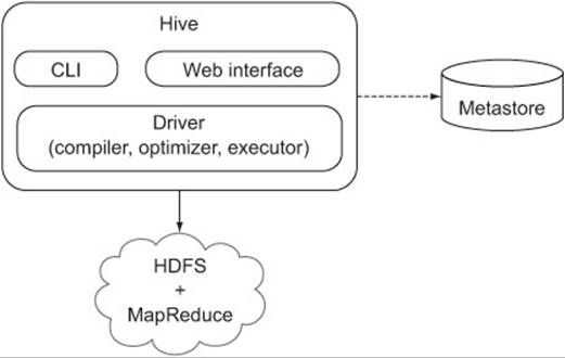
Hive was originally an internal Facebook project that eventually tenured into a full-blown Apache project. It was created to simplify access to MapReduce by exposing a SQL-based language for data manipulation. The Hive architecture can be seen in figure 9.1.

Figure 9.1. The Hive high-level architecture

In this chapter we’ll look at practical examples of how you can use Hive to work with Apache web server logs. We’ll look at different ways you can load and arrange data in Hive to optimize how you access that data. We’ll also look at some advanced join mechanisms and other relational operations such as grouping and sorting. We’ll kick things off with a brief introduction to Hive.

Learning more about Hive basics

To fully understand Hive fundamentals, refer to Chuck Lam’s Hadoop in Action (Manning, 2010). In this section we’ll just skim through some Hive basics.

9.1.1. Hive basics

Let’s quickly look at some Hive basics, including recent developments in its execution framework.

Installing Hive

The appendix contains installation instructions for Hive. All the examples in this book were executed on Hive 0.13, and it’s possible some older Hive versions don’t support some of the features we’ll use in this book.

The Hive metastore

Hive maintains metadata about Hive in a metastore, which is stored in a relational database. This metadata contains information about what tables exist, their columns, user privileges, and more.

By default, Hive uses Derby, an embedded Java relational database, to store the metastore. Because it’s embedded, Derby can’t be shared between users, and as such it can’t be used in a multi-user environment where the metastore needs to be shared.

Databases, tables, partitions, and storage

Hive can support multiple databases, which can be used to avoid table-name collisions (two teams or users that have the same table name) and to allow separate databases for different users or products.

A Hive table is a logical concept that’s physically composed of a number of files in HDFS. Tables can either be internal, where Hive organizes them inside a warehouse directory (controlled by the hive.metastore.warehouse.dir property with a default value of /user/hive/warehouse [in HDFS]), or they can be external, in which case Hive doesn’t manage them. Internal tables are useful if you want Hive to manage the complete lifecycle of your data, including the deletion, whereas external tables are useful when the files are being used outside of Hive.

Tables can be partitioned, which is a physical arrangement of data, into distinct subdirectories for each unique partitioned key. Partitions can be static and dynamic, and we’ll look at both cases in technique 92.

Hive’s data model

Hive supports the following data types:

· Signed integers —BIGINT (8 bytes), INT (4 bytes), SMALLINT (2 bytes), and TINYINT (1 byte)

· Floating-point numbers —FLOAT (single precision) and DOUBLE (double precision)

· Booleans —TRUE or FALSE

· Strings —Sequences of characters in specified character sets

· Maps —Associative arrays with collections of key/value pairs where keys are unique

· Arrays —Indexable lists, where all elements must be of the same type

· Structs —Complex types that contain elements

Hive’s query language

Hive’s query language supports much of the SQL specification, along with Hive-specific extensions, some of which are covered in this section. The full list of statements supported in Hive can be viewed in the Hive Language Manual:https://cwiki.apache.org/confluence/display/Hive/LanguageManual.

Tez

On Hadoop 1, Hive was limited to using MapReduce to execute most of the statements because MapReduce was the only processing engine supported on Hadoop. This wasn’t ideal, as users coming to Hive from other SQL systems were used to highly interactive environments where queries are frequently completed in seconds. MapReduce was designed for high-throughput batch processing, so its startup overhead coupled with its limited processing capabilities resulted in very high-latency query executions.

With the Hive 0.13 release, Hive now uses Tez on YARN to execute its queries, and as a result, it’s able to get closer to the interactive ideal for working with your data.^[¹^] Tez is basically a generalized Directed Acyclic Graph (DAG) execution engine that doesn’t impose any limits on how you compose your execution graph (as opposed to MapReduce) and that also allows you to keep data in-memory in between phases, reducing the disk and network I/O that MapReduce requires. You can read more about Tez at the following links:

¹ Carter Shanklin, “Benchmarking Apache Hive 13 for Enterprise Hadoop,” http://hortonworks.com/blog/benchmarking-apache-hive-13-enterprise-hadoop/.

· Hive on Tez: https://cwiki.apache.org/confluence/display/Hive/Hive+on+Tez

· Tez incubation Apache project page: http://incubator.apache.org/projects/tez.html

In the Hive 0.13 release, Tez isn’t enabled by default, so you’ll need to follow these instructions to get it up and running:

· Tez installation instructions: https://github.com/apache/incubator-tez/blob/branch-0.2.0/INSTALL.txt

· Configuring Hive to work on Tez: https://issues.apache.org/jira/browse/HIVE-6098

Interactive and non-interactive Hive

The Hive shell provides an interactive interface:

$ hive

hive> SHOW DATABASES;

default

Time taken: 0.162 seconds

Hive in non-interactive mode lets you execute scripts containing Hive commands. The following example uses the -S option so that only the output of the Hive command is written to the console:

$ cat hive-script.ql

SHOW DATABASES;

$ hive -S -f hive-script.ql

default

Another non-interactive feature is the -e option, which lets you supply a Hive command as an argument:

$ hive -S -e "SHOW DATABASES"

default

If you’re debugging something in Hive and you want to see more detailed output on the console, you can use the following command to run Hive:

$ hive -hiveconf hive.root.logger=INFO,console

That concludes our brief introduction to Hive. Next we’ll look at how you can use Hive to mine interesting data from your log files.

9.1.2. Reading and writing data

This section covers some of the basic data input and output mechanics in Hive. We’ll ease into things with a brief look at working with text data before jumping into how you can work with Avro and Parquet data, which are becoming common ways to store data in Hadoop.

This section also covers some additional data input and output scenarios, such as writing and appending to tables and exporting data out to your local filesystem. Once we’ve covered these basic functions, subsequent sections will cover more advanced topics such as writing UDFs and performance tuning tips.

Technique 89 Working with text files

Imagine that you have a number of CSV or Apache log files that you want to load and analyze using Hive. After copying them into HDFS (if they’re not already there), you’ll need to create a Hive table before you can issue queries. If the result of your work is also large, you may want to write it into a new Hive table. This section covers these text I/O use cases in Hive.

Problem

You want to use Hive to load and analyze text files, and then save the results.

Solution

Use the RegexSerDe class, bundled with the contrib library in Hive, and define a regular expression that can be used to parse the contents of Apache log files. This technique also looks at how serialization and deserialization works in Hive, and how to write your own SerDe to work with log files.

Discussion

If you issue a CREATE TABLE command without any row/storage format options, Hive assumes the data is text-based using the default line and field delimiters shown in table 9.1.

Table 9.1. Default text file delimiters

Default delimiter	Syntax example to change default delimiter	Description
\n	LINES TERMINATED BY '\n'	Record separator.
^A	FIELDS TERMINATED BY '\t'	Field separator. If you wanted to replace ^A with another non-readable character, you’d represent it in octal, e.g., '\001'.
^B	COLLECTION ITEMS TERMINATED BY ';'	An element separator for ARRAY, STRUCT, and MAP data types.
^C	MAP KEYS TERMINATED BY ':'	Used as a key/value separator in MAP data types.

Because most of the text data that you’ll work with will be structured in more standard ways, such as CSV, let’s look at how you can work with CSV.

First you’ll need to copy the stocks CSV file included with the book’s code into HDFS. Create a directory in HDFS and then copy the stocks file into the directory:^[²^]

² Hive doesn’t allow you to create a table over a file; it must be a directory.

$ hadoop fs -mkdir hive-stocks

$ hadoop fs -put test-data/stocks.txt hive-stocks

Now you can create an external Hive table over your stocks directory:

hive> CREATE EXTERNAL TABLE stocks (

symbol STRING,

date STRING,

open FLOAT,

high FLOAT,

low FLOAT,

close FLOAT,

volume INT,

adj_close FLOAT

)

ROW FORMAT DELIMITED FIELDS TERMINATED BY ','

LOCATION '/user/YOUR-USERNAME/hive-stocks';

Creating managed tables with the LOCATION keyword

When you create an external (unmanaged) table, Hive keeps the data in the directory specified by the LOCATION keyword intact. But if you were to execute the same CREATE command and drop the EXTERNAL keyword, the table would be a managed table, and Hive would move the contents of the LOCATION directory into /user/hive/warehouse/stocks, which may not be the behavior you expect.

Run a quick query to verify that things look good:

hive> SELECT symbol, count(*) FROM stocks GROUP BY symbol;

AAPL 10

CSCO 10

GOOG 5

MSFT 10

YHOO 10

Sweet! What if you wanted to save the results into a new table and then show the schema of the new table?

hive> CREATE TABLE symbol_counts

ROW FORMAT DELIMITED FIELDS TERMINATED BY ','

LOCATION '/user/YOUR-USERNAME/symbol_counts'

AS SELECT symbol, count(*) FROM stocks GROUP BY symbol;

hive> describe symbol_counts;

symbol string

Create-Table-As-Select (CTAS) and external tables

CAS statements like the preceding example don’t allow you to specify that the table is EXTERNAL. But because the table that you’re selecting from is already an external table, Hive ensures that the new table is also an external table.

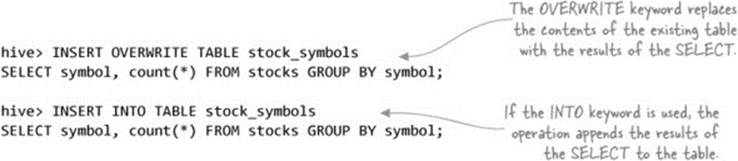
If the target table already exists, you have two options—you can either overwrite the entire contents of the table, or you can append to the table:

You can view the raw table data using the Hadoop CLI:

$ hdfs -cat symbol_counts/*

AAPL,10

CSCO,10

GOOG,5

MSFT,10

YHOO,10

The great thing about Hive external tables is that you can write into them using any method (it doesn’t have to be via a Hive command), and Hive will automatically pick up the additional data the next time you issue any Hive statements.

Tokenizing files with regular expressions

Let’s make things more complicated and assume you want to work with log data. This data is in text form, but it can’t be parsed using Hive’s default deserialization. Instead, you need a way to specify a regular expression to parse your log data. Hive comes with a contrib RegexSerDe class that can tokenize your logs.

First, copy some log data into HDFS:

$ hadoop fs -mkdir log-data

$ hadoop fs -put test-data/ch9/hive-log.txt log-data/

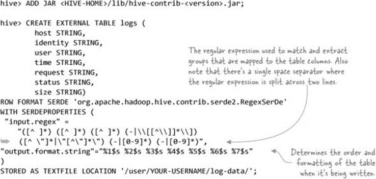
Next, specify that you want to use a custom deserializer. The RegexSerDe is bundled with the Hive contrib JAR, so you’ll need to add this JAR to Hive:

A quick test will tell you if the data is being correctly handled by the SerDe:

hive> SELECT host, request FROM logs LIMIT 10;

89.151.85.133 "GET /movie/127Hours HTTP/1.1"

212.76.137.2 "GET /movie/BlackSwan HTTP/1.1"

74.125.113.104 "GET /movie/TheFighter HTTP/1.1"

212.76.137.2 "GET /movie/Inception HTTP/1.1"

127.0.0.1 "GET /movie/TrueGrit HTTP/1.1"

10.0.12.1 "GET /movie/WintersBone HTTP/1.1"

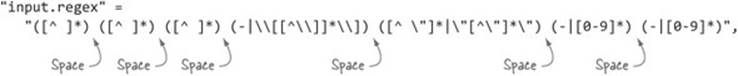
If you’re seeing nothing but NULL values in the output, it’s probably because you have a missing space in your regular expression. Ensure that the regex in the CREATE statement looks like figure 9.2.

Figure 9.2. CREATE table regex showing spaces

Hive’s SerDe is a flexible mechanism that can be used to extend Hive to work with any file format, as long as an InputFormat exists that can work with that file format. For more details on SerDes, take a look at the Hive documentation athttps://cwiki.apache.org/confluence/display/Hive/SerDe.

Working with Avro and Parquet

Avro is an object model that simplifies working with your data, and Parquet is a columnar storage format that can efficiently support advanced query optimizations such as predicate pushdowns. Combined, they’re a compelling pair and could well become the canonical way that data is stored in Hadoop. We covered both Avro and Parquet in depth in chapter 3, which in technique 23 shows you how to use Avro and Parquet in Hive.

Technique 90 Exporting data to local disk

Getting data out of Hive and Hadoop is an important function you’ll need to be able to perform when you have data that you’re ready to pull into your spreadsheets or other analytics software. This technique examines a few methods you can use to pull out your Hive data.

Problem

You have data sitting in Hive that you want to pull out to your local filesystem.

Solution

Use the standard Hadoop CLI tools or a Hive command to pull out your data.

Discussion

If you want to pull out an entire Hive table to your local filesystem and the data format that Hive uses for your table is the same format that you want your data exported in, you can use the Hadoop CLI and run a hadoop -get /user/hive/warehouse/... command to pull down the table.

Hive comes with EXPORT (and corresponding IMPORT) commands that can be used to export Hive data and metadata into a directory in HDFS. This is useful for copying Hive tables between Hadoop clusters, but it doesn’t help you much in getting data out to the local filesystem.

If you want to filter, project, and perform some aggregations on your data and then pull it out of Hive, you can use the INSERT command and specify that the results should be written to a local directory:

hive> INSERT OVERWRITE LOCAL DIRECTORY 'local-stocks' SELECT * FROM stocks;

This will create a directory on your local filesystem containing one or more files. If you view the files in an editor such as vi, you’ll notice that Hive used the default field separator (^A) when writing the files. And if any of the columns you exported were complex types (such as STRUCT or MAP), then Hive will use JSON to encode these columns.

Luckily, newer versions of Hive (including 0.13) allow you to specify a custom delimiter when you export tables:

hive> INSERT OVERWRITE LOCAL DIRECTORY 'local-stocks'

ROW FORMAT DELIMITED FIELDS TERMINATED BY ','

SELECT * FROM stocks;

With Hive’s reading and writing basics out of the way, let’s take a look at more complex topics, such as user-defined functions.

9.1.3. User-defined functions in Hive

We’ve looked at how Hive reads and writes tables, so it’s time to start doing something useful with your data. Since we want to cover more advanced techniques, we’ll look at how you can write a custom Hive user-defined function (UDF) to geolocate your logs. UDFs are useful if you want to mix custom code inline with your Hive queries.

Technique 91 Writing UDFs

This technique shows how you can write a Hive UDF and then use it in your Hive Query Language (HiveQL).

Problem

How do you write a custom function in Hive?

Solution

Extend the UDF class to implement your user-defined function and call it as a function in your HiveQL.

Discussion

You can geolocate the IP addresses from the logs table using the free geolocation database from MaxMind.

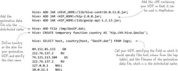
Download the free country geolocation database,^[³^] gunzip it, and copy the GeoIP.dat file to your /tmp/ directory. Next, use a UDF to geolocate the IP address from the log table that you created in technique 89:

³ See MaxMind’s “GeoIP Country Database Installation Instructions,” http://dev.maxmind.com/geoip/legacy/install/country/.

When writing a UDF, there are two implementation options: either extend the UDF class or implement the GenericUDF class. The main differences between them are that the GenericUDF class can work with arguments that are complex types, so UDFs that extend GenericUDF are more efficient because the UDF class requires Hive to use reflection for discovery and invocation. Figure 9.3 shows the two Hive UDF classes, one of which you need to extend to implement your UDF.

Figure 9.3. Hive UDF class diagram

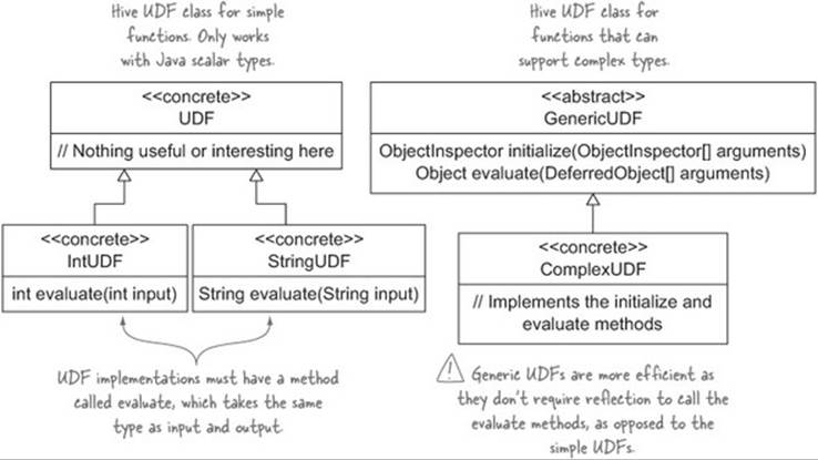
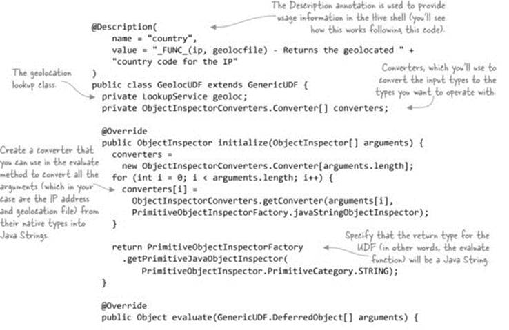
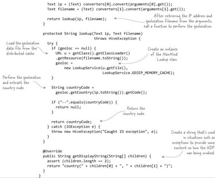
The following listing shows the geolocation UDF, which you’ll implement using the GenericUDF class.^[⁴^]

⁴ GitHub source: https://github.com/alexholmes/hiped2/blob/master/src/main/java/hip/ch9/hive/Geoloc.java.

Listing 9.1. The geolocation UDF

The Description annotation can be viewed in the Hive shell with the describe function command:

hive> describe function country;

country(ip, geolocfile) - Returns the geolocated country code

for the IP

Summary

Although the UDF we looked at operates on scalar data, Hive also has something called user-defined aggregate functions (UDAF), which allows more complex processing capabilities over aggregated data. You can see more about writing a UDAF on the Hive wiki at the page titled “Hive Operators and User-Defined Functions (UDFs)” (https://cwiki.apache.org/confluence/display/Hive/LanguageManual+UDF).

Hive also has user-defined table functions (UDTFs), which operate on scalar data but can emit more than one output for each input. See the GenericUDTF class for more details.

Next we’ll take a look at what you can do to optimize your workflows in Hive.

9.1.4. Hive performance

In this section, we’ll examine some methods that you can use to optimize data management and processing in Hive. The tips presented here will help you ensure that as you scale out your data, the rest of Hive will keep up with your needs.

Technique 92 Partitioning

Partitioning is a common technique employed by SQL systems to horizontally or vertically split data to speed up data access. With reduced overall volume of data in a partition, partitioned read operations have a lot less data to sift through, and as a result can execute much more rapidly.

This same principle applies equally well to Hive, and it becomes increasingly important as your data sizes grow. In this section you’ll explore the two types of partitions in Hive: static partitions and dynamic partitions.

Problem

You want to arrange your Hive files so as to optimize queries against your data.

Solution

Use PARTITIONED BY to partition by columns that you typically use when querying your data.

Discussion

Imagine you’re working with log data. A natural way to partition your logs would be by date, allowing you to perform queries on specific time periods without incurring the overhead of a full table scan (reading the entire contents of the table). Hive supports partitioned tables and gives you control of determining which columns are partitioned.

Hive supports two types of partitions: static partitions and dynamic partitions. They differ in the way you construct INSERT statements, as you’ll discover in this technique.

Static partitioning

For the purpose of this technique, you’ll work with a very simple log structure. The fields are IP address, year, month, day, and HTTP status code:

$ cat test-data/ch9/logs-partition.txt

127.0.0.1,2014,06,21,500

127.0.0.1,2014,06,21,400

127.0.0.1,2014,06,21,300

127.0.0.1,2014,06,22,200

127.0.0.1,2014,06,22,210

127.0.0.1,2014,06,23,100

Load them into HDFS and into an external table:

$ hadoop fs -mkdir logspartext

$ hadoop fs -put test-data/ch9/logs-partition.txt logspartext/

hive> CREATE EXTERNAL TABLE logs_ext (

ip STRING,

year INT,

month INT,

day INT,

status INT

)

ROW FORMAT DELIMITED FIELDS TERMINATED BY ','

LOCATION '/user/YOUR-USERNAME/logspartext';

Now you can create a partitioned table, where the year, month, and day are partitions:

CREATE EXTERNAL TABLE IF NOT EXISTS logs_static (

ip STRING,

status INT)

PARTITIONED BY (year INT, month INT, day INT)

ROW FORMAT DELIMITED FIELDS TERMINATED BY '\t'

LOCATION '/user/YOUR-USERNAME/logs_static';

By default, Hive inserts follow a static partition method that requires all inserts to explicitly enumerate not only the partitions, but the column values for each partition. Therefore, an individual INSERT statement can only insert into one day’s worth of partitions:

INSERT INTO TABLE logs_static

PARTITION (year = '2014', month = '06', day = '21')

SELECT ip, status FROM logs_ext WHERE year=2014 AND month=6 AND day=21;

Luckily Hive has a special data manipulation language (DML) statement that allows you to insert into multiple partitions in a single statement. The following code will insert all the sample data (spanning three days) into the three partitions:

FROM logs_ext se

INSERT INTO TABLE logs_static

PARTITION (year = '2014', month = '6', day = '21')

SELECT ip, status WHERE year=2014 AND month=6 AND day=21

INSERT INTO TABLE logs_static

PARTITION (year = '2014', month = '6', day = '22')

SELECT ip, status WHERE year=2014 AND month=6 AND day=22

INSERT INTO TABLE logs_static

PARTITION (year = '2014', month = '6', day = '23')

SELECT ip, status WHERE year=2014 AND month=6 AND day=23;

This approach has an additional advantage in that it will only make one pass over the logs_ext table to perform the inserts—the previous approach would have required N queries on the source table for N partitions.

Flexibility of single-pass static partitioned inserts

Hive doesn’t limit either the destination tables or whether the query conditions need to align with the partitions. Therefore, there’s nothing stopping you from inserting into different tables and having overlapping rows in multiple partitions or tables.

One disadvantage of static partitions is that when you’re inserting data, you must explicitly specify the partition that’s being inserted into. But you’re not stuck with static partitions as the only partitions supported in Hive. Hive has the notion of dynamic partitions, which make life a little easier by not requiring you to specify the partition when inserting data.

Dynamic partitioning

Dynamic partitions are smarter than static partitions, as they can automatically determine which partition a record needs to be written to when data is being inserted.

Let’s create a whole new table to store some dynamic partitions. Notice how the syntax to create a table that uses dynamic partitions is exactly the same as that for static partitioned tables:

CREATE EXTERNAL TABLE IF NOT EXISTS logs_dyn (

ip STRING,

status INT)

PARTITIONED BY (year INT, month INT, day INT)

ROW FORMAT DELIMITED FIELDS TERMINATED BY '\t'

LOCATION '/user/YOUR-USERNAME/logs_dyn';

The differences only come into play at INSERT time:

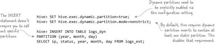
That’s a lot better—you no longer need to explicitly tell Hive which partitions you’re inserting into. It’ll dynamically figure this out.

Mixing dynamic and static partitions in the same table

Hive supports mixing both static and dynamic columns in a table. There’s also nothing stopping you from transitioning from a static partition insert method to dynamically partitioned inserts.

Partition directory layout

Partitioned tables are laid out in HDFS differently from nonpartitioned tables. Each partition value occupies a separate directory in Hive containing the partition column name as well as its value.

These are the contents of HDFS after running the most recent INSERT:

logs_static/year=2014/month=6/day=21/000000_0

logs_static/year=2014/month=6/day=22/000000_0

logs_static/year=2014/month=6/day=23/000000_0

The “000000_0” are the files that contain the rows. There’s only one per partitioned day due to the small dataset (running with a larger dataset with more than one task will result in multiple files).

Customizing partition directory names

As you just saw, left to its own devices, Hive will create partition directory names using the column=value format. What if you wanted to have more control over the directories? Instead of your partitioned directory looking like this,

logs_static/year=2014/month=6/day=27

what if you wanted it to look like this:

logs_static/2014/6/27

You can achieve this by giving Hive the complete path that should be used to store a partition:

ALTER TABLE logs_static

ADD PARTITION(year=2014, month=6, day=27)

LOCATION '/user/YOUR-USERNAME/logs_static/2014/6/27';

You can query the location of individual partitions with the DESCRIBE command:

hive> DESCRIBE EXTENDED logs_static

PARTITION (year=2014, month=6, day=28);

...

location:hdfs://localhost:8020/user/YOUR-USERNAME/logs_static/2014/6/27

...

This can be a powerful tool, as Hive doesn’t require that all the partitions for a table be on the same cluster or type of filesystem. Therefore, a Hive table could have a partition sitting in Hadoop cluster A, another sitting in cluster B, and a third in a cluster in Amazon S3. This opens up some powerful strategies for aging out data to other filesystems.

Querying partitions from Hive

Hive provides some commands to allow you to see the current partitions for a table:

hive> SHOW PARTITIONS logs_dyn;

year=2014/month=6/day=21

year=2014/month=6/day=22

year=2014/month=6/day=23

Bypassing Hive to load data into partitions

Let’s say you had some data for a new partition (2014/6/24) that you wanted to manually copy into your partitioned Hive table using HDFS commands (or some other mechanism such as MapReduce).

Here’s some sample data (note that the date parts are removed because Hive only retains these column details in the directory names):

$ cat test-data/ch9/logs-partition-supplemental.txt

127.0.0.1 500

127.0.0.1 600

Create a new partitioned directory and copy the file into it:

$ hdfs -mkdir logs_dyn/year=2014/month=6/day=24

$ hdfs -put test-data/ch9/logs-partition-supplemental.txt \

logs_dyn/year=2014/month=6/day=24

Now go to your Hive shell and try to select the new data:

hive> SELECT * FROM logs_dyn

WHERE year = 2014 AND month = 6 AND day = 24;

No results! This is because Hive doesn’t yet know about the new partition. You can run a repair command so that Hive can examine HDFS to determine the current partitions:

hive> msck repair table logs_dyn;

Partitions not in metastore: logs_dyn:year=2014/month=6/day=24

Repair: Added partition to metastore logs_dyn:year=2014/month=6/day=24

Now your SELECT will work:

hive> SELECT * FROM logs_dyn

WHERE year = 2014 AND month = 6 AND day = 24;

127.0.0.1 500 2014 6 24

127.0.0.1 600 2014 6 24

Alternatively, you could explicitly inform Hive about the new partition:

ALTER TABLE logs_dyn

ADD PARTITION (year=2014, month=6, day=24);

Summary

Given the flexibility of dynamic partitions, in what situations would static partitions offer an advantage? One example is in cases where the data that you’re inserting doesn’t have any knowledge of the partitioned columns, but some other process does.

For example, suppose you have some log data that you want to insert, but for whatever reason the log data doesn’t contain dates. In this case, you can craft a static partitioned insert as follows:

$ hive -hiveconf year=2014 -hiveconf month=6 -hiveconf day=28

hive> INSERT INTO TABLE logs_static

PARTITION (year=${hiveconf:year},

month=${hiveconf:month},

day=${hiveconf:day})

SELECT ip, status FROM logs_ext;

Let’s next take a look at columnar data, which is another form of data partitioning that can provide dramatic query execution time improvements.

Columnar data

Most data that we’re used to working with is stored on disk in row-oriented order, meaning that all the columns for a row are contiguously located when stored at rest on persistent storage. CSV, SequenceFiles, and Avro are typically stored in rows.

Using a column-oriented storage format for saving your data can offer huge performance benefits, both from space and execution-time perspectives. Contiguously locating columnar data together allows storage formats to use sophisticated data-compression schemes such as run-length encoding, which can’t be applied to row-oriented data. Furthermore, columnar data allows execution engines such as Hive, Map-Reduce, and Tez to push predicates and projections to the storage formats, allowing these storage formats to skip over data that doesn’t match the pushdown criteria.

There are currently two hot options for columnar storage on Hive (and Hadoop): Optimized Row Columnar (ORC) and Parquet. They come out of Hortonworks and Cloudera/Twitter, respectively, and both offer very similar space- and time-saving optimizations. The only edge really comes out of the goal of Parquet to maximize compatibility in the Hadoop community, so at the time of writing, Parquet has greater support for the Hadoop ecosystem.

Chapter 3 has a section devoted to Parquet, and technique 23 includes instructions on how Parquet can be used with Hive.

Technique 93 Tuning Hive joins

It’s not uncommon to execute a join over some large datasets in Hive and wait hours for it to complete. In this technique we’ll look at how joins can be optimized, much like we did for MapReduce in chapter 4.

Problem

Your Hive joins are running slower than expected, and you want to learn what options you have to speed them up.

Solution

Look at how you can optimize Hive joins with repartition joins, replication joins, and semi-joins.

Discussion

We’ll cover three types of joins in Hive: the repartition join, which is the standard reduce-side join; the replication join, which is the map-side join; and the semi-join, which only cares about retaining data from one table.

Before we get started, let’s create two tables to work with:

$ hadoop fs -mkdir stocks-mini

$ hadoop fs -put test-data/ch9/stocks-mini.txt stocks-mini

$ hadoop fs -mkdir symbol-names

$ hadoop fs -put test-data/ch9/symbol-names.txt symbol-names

hive> CREATE EXTERNAL TABLE stocks (

symbol STRING,

date STRING,

open FLOAT

)

ROW FORMAT DELIMITED FIELDS TERMINATED BY ','

LOCATION '/user/YOUR-USERNAME/stocks-mini';

hive> CREATE EXTERNAL TABLE names (

symbol STRING,

name STRING

)

ROW FORMAT DELIMITED FIELDS TERMINATED BY ','

LOCATION '/user/YOUR-USERNAME/symbol-names';

You’ve created two tables. The stocks table contains just three columns—the stock symbol, the date, and the price. The names table contains the stock symbols and the company names:

hive> select * from stocks;

AAPL 2009-01-02 85.88

AAPL 2008-01-02 199.27

CSCO 2009-01-02 16.41

CSCO 2008-01-02 27.0

GOOG 2009-01-02 308.6

GOOG 2008-01-02 692.87

MSFT 2009-01-02 19.53

MSFT 2008-01-02 35.79

YHOO 2009-01-02 12.17

YHOO 2008-01-02 23.8

hive> select * from names;

AAPL Apple

GOOG Google

YHOO Yahoo!

Join table ordering

As with any type of tuning, it’s important to understand the internal workings of a system. When Hive executes a join, it needs to select which table is streamed and which table is cached. Hive picks the last table in the JOIN statement for streaming, so you should take care to ensure that this is the largest table.

Let’s look at the example of our two tables. The stocks table, which includes daily quotes, will continue to grow over time, but the names table, which contains the stock symbol names, will be mostly static. Therefore, when these tables are joined, it’s important that the larger table, stocks, comes last in the query:

SELECT stocks.symbol, date, open, name

FROM names

JOIN stocks ON (names.symbol = stocks.symbol);

You can also explicitly tell Hive which table it should stream:

SELECT /*+ STREAMTABLE(stocks) */ stocks.symbol, date, open, name

FROM names

JOIN stocks ON (names.symbol = stocks.symbol);

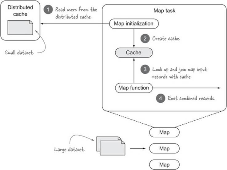
Map-side joins

A replicated join is a map-side join where a small table is cached in memory and the large table is streamed. You can see how it works in MapReduce in figure 9.4.

Figure 9.4. A replicated join

Map-side joins can be used to execute both inner and outer joins. The current recommendation is that you configure Hive to automatically attempt to convert joins into map-side joins:

hive> set hive.auto.convert.join = true;

hive> SET hive.auto.convert.join.noconditionaltask = true;

hvie> SET hive.auto.convert.join.noconditionaltask.size = 10000000;

The first two settings must be set to true to enable autoconversion of joins to map-side joins (in Hive 0.13 they’re both enabled by default). The last setting is used by Hive to determine whether a join can be converted. Imagine you have N tables in your join. If the size of the smallest N – 1 tables on disk is less than hive.auto.convert.join.noconditionaltask.size, then the join is converted to a map-side join. Bear in mind that the check is rudimentary and only examines the size of the tables on disk, so factors such as compression and filters or projections don’t come into the equation.

Map-join hint

Older versions of Hive supported a hint that you could use to instruct Hive which table was the smallest and should be cached. Here’s an example:

SELECT /*+ MAPJOIN(names) */ stocks.symbol, date, open, name

FROM names

JOIN stocks ON (names.symbol = stocks.symbol);

Recent versions of Hive ignore this hint (hive.ignore.mapjoin.hint is set to true by default) because it put the onus on the query author to determine the smaller table, which can lead to slow queries due to user error.

Sort-merge-bucket joins

Hive tables can be bucketed and sorted, which helps you to easily sample data, and it’s also a useful join optimization as it enables sort-merge-bucket (SMB) joins. SMB joins require that all tables be sorted and bucketed, in which case joins are very efficient because they require a simple merge of the presorted tables.

The following example shows how you’d create a sorted and bucketed stocks table:

CREATE TABLE stocks_bucketed (

symbol STRING,

date STRING,

open FLOAT

)

CLUSTERED BY(symbol) SORTED BY(symbol) INTO 32 BUCKETS;

Inserting into bucketed tables

You can use regular INSERT statements to insert into bucketed tables, but you need to set the hive.enforce.bucketing property to true. This instructs Hive that it should look at the number of buckets in the table to determine the number of reducers that will be used when inserting into the table (the number of reducers must be equal to the number of buckets).

To enable SMB joins, you must set the following properties:

set hive.auto.convert.sortmerge.join=true;

set hive.optimize.bucketmapjoin = true;

set hive.optimize.bucketmapjoin.sortedmerge = true;

set hive.auto.convert.sortmerge.join.noconditionaltask=true;

In addition, you’ll also need to ensure that the following conditions hold true:

· All tables being joined are bucketed and sorted on the join column.

· The number of buckets in each join table must be equal, or factors of one another.

Skew

Skew can lead to lengthy MapReduce execution times because a small number of reducers may receive a disproportionately large number of records for some join values. Hive, by default, doesn’t attempt to do anything about this, but it can be configured to detect skew and optimize joins on skewed keys:

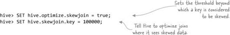
So what happens when Hive detects skew? You can see the additional step that Hive adds in figure 9.5, where skewed keys are written to HDFS and processed in a separate MapReduce job.

Figure 9.5. Hive skew optimization

It should be noted that this skew optimization only works with reduce-side repartition joins, not map-side replication joins.

Skewed tables

If you know ahead of time that there are particular keys with high skews, you can tell Hive about them when creating your table. If you do this, Hive will write out skewed keys into separate files that allow it to further optimize queries, and even to skip over the files if possible.

Imagine that you have two stocks (Apple and Google) that have a much larger number of records compared to the others—in this case you’d modify your CREATE TABLE statement with the keywords SKEWED BY, as follows:

CREATE TABLE stocks_skewed (

symbol STRING,

date STRING,

open FLOAT

)

SKEWED BY (symbol) ON ('AAPL', 'GOOGL');

9.2. Impala

Impala is a low-latency, massively parallel query engine, modeled after Google’s Dremel paper describing a scalable and interactive query system.^[⁵^] Impala was conceived and developed out of Cloudera, which realized that using MapReduce to execute SQL wasn’t viable for a low-latency SQL environment.

⁵ Sergey Melnik et al., “Dremel: Interactive Analysis of Web-Scale Datasets,” http://research.google.com/pubs/pub36632.html.

Each daemon in Impala is designed to be self-sufficient, and a client can send a query to any Impala daemon. Impala does have some metadata services, but it can continue to function even when they’re not working, as the daemon nodes talk directly to one another to execute queries. An overview of the Impala architecture can be seen in figure 9.6.

Figure 9.6. The Impala architecture

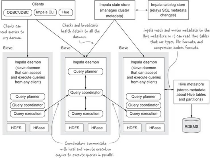
Impala allows you to query data in HDFS or HBase with a SQL syntax, so it supports access via ODBC. It uses the Hive metastore, so it can read existing Hive tables, and DDL statements executed via Impala are also reflected in Hive.

In this section I’ll present some of the differences between Impala and Hive, and we’ll also look at some basic examples of Impala in action, including how Hive UDFs can be used.

9.2.1. Impala vs. Hive

There are a handful of differences between Impala and Hive:

· Impala is designed from the ground up as a massively parallel query engine and doesn’t need to translate SQL into another processing framework. Hive relies on MapReduce (or more recently Tez) to execute.

· Impala and Hive are both open source, but Impala is a curated project under Cloudera’s control.

· Impala isn’t fault-tolerant.

· Impala doesn’t support complex types such as maps, arrays, and structs (including nested Avro data). You can basically only work with flat data.^[⁶^]

⁶ Impala and Avro nested type support is planned for Impala 2.0: https://issues.cloudera.org/browse/IMPALA-345.

· There are various file formats and compression codec combinations that require you to use Hive to create and load tables. For example, you can’t create or load data into an Avro table in Impala, and you can’t load an LZO-compressed text file in Impala. For Avro you need to create the table in Hive before you can use it in Impala, and in both Avro and LZO-compressed text, you’ll need to load your data into these tables using Hive before you can use them in Impala.

· Impala doesn’t support Hive user-defined table-generating functions (UDTSs), although it does support Hive UDFs and UDAFs and can work with existing JARs that contain these UDFs without any changes to the JAR.

· There are certain aggregate functions and HiveQL statements that aren’t supported in Impala.

Impala and Hive versions

This list compares Hive 0.13 and Impala 1.3.1, both of which are current at the time of writing. It should be noted that the Impala 2 release will address some of these items.

Cloudera has a detailed list of the SQL differences between Impala and Hive: http://mng.bz/0c2F.

9.2.2. Impala basics

This section covers what are likely the two most popular data formats for Impala—text and Parquet.

Technique 94 Working with text

Text is typically the first file format that you’ll work with when exploring a new tool, and it also serves as a good learning tool for understanding the basics.

Problem

You have data in text form that you want to work with in Impala.

Solution

Impala’s text support is identical to Hive’s.

Discussion

Impala’s basic query language is identical to Hive’s. Let’s kick things off by copying the stocks data into a directory in HDFS:

$ hadoop fs -mkdir hive-stocks

$ hadoop fs -put test-data/stocks.txt hive-stocks

Next you’ll create an external table and run a simple aggregation over the data:

$ impala-shell

> CREATE EXTERNAL TABLE stocks (

sym STRING,

dt STRING,

open FLOAT,

high FLOAT,

low FLOAT,

close FLOAT,

volume INT,

adj_close FLOAT

)

ROW FORMAT DELIMITED FIELDS TERMINATED BY ','

LOCATION '/user/YOUR-USERNAME/hive-stocks';

> SELECT sym, min(close), max(close) FROM stocks GROUP BY sym;

+------+-------------------+-------------------+

| sym | min(close) | max(close) |

+------+-------------------+-------------------+

| MSFT | 20.32999992370605 | 116.5599975585938 |

| AAPL | 14.80000019073486 | 194.8399963378906 |

| GOOG | 202.7100067138672 | 685.1900024414062 |

| CSCO | 13.64000034332275 | 108.0599975585938 |

| YHOO | 12.85000038146973 | 475 |

+------+-------------------+-------------------+

Using Hive tables in Impala

The example in technique 94 shows how to create a table called stocks in Impala. If you’ve already created the stocks table in Hive (as shown in technique 89), then rather than create the table in Impala, you should refresh Impala’s metadata and then use that Hive table in Impala.

After creating the table in Hive, issue the following statement in the Impala shell:

> INVALIDATE METADATA stocks;

At this point, you can issue queries against the stocks table inside the Impala shell.

Alternatively, if you really want to create the table in Impala and you’ve already created the table in Hive, you’ll need to issue a DROP TABLE command prior to issuing the CREATE TABLE command in Impala.

That’s it! You’ll notice that the syntax is exactly the same as in Hive. The one difference is that you can’t use symbol and date as column names because they’re reserved symbols in Impala (Hive doesn’t have any such restrictions).

Let’s take a look at working with a storage format that’s a bit more interesting: Parquet.

Technique 95 Working with Parquet

It’s highly recommended that you use Parquet as your storage format for various space and time efficiencies (see chapter 3 for more details on Parquet’s benefits). This technique looks at how you can create Parquet tables in Impala.

Problem

You need to save your data in Parquet format to speed up your queries and improve the compression of your data.

Solution

Use STORED AS PARQUET when creating tables.

Discussion

One way to get up and started quickly with Parquet is to create a new Parquet table based on an existing table (the existing table doesn’t need to be a Parquet table). Here’s an example:

CREATE TABLE stocks_parquet LIKE stocks STORED AS PARQUET;

Then you can use an INSERT statement to copy the contents from the old table into the new Parquet table:

INSERT OVERWRITE TABLE stocks_parquet SELECT * FROM stocks;

Now you can ditch your old table and start using your shiny new Parquet table!

> SHOW TABLE STATS stocks_parquet;

Query: show TABLE STATS stocks_parquet

+-------+--------+--------+---------+

+-------+--------+--------+---------+

| -1 | 1 | 2.56KB | PARQUET |

+-------+--------+--------+---------+

Alternatively, you can create a new table from scratch:

CREATE TABLE stocks_parquet_internal (

sym STRING,

dt STRING,

open DOUBLE,

high DOUBLE,

low DOUBLE,

close DOUBLE,

volume INT,

adj_close DOUBLE

) STORED AS PARQUET;

One of the great things about Impala is that it allows the INSERT ... VALUES syntax, so you can easily get data into the table:^[⁷^]

⁷ The use of INSERT ... VALUES isn’t recommended for large data loads. Instead, it’s more efficient to move files into your table’s HDFS directory, use the LOAD DATA statement, or use INSERT INTO ... SELECT or CREATE TABLE AS SELECT ... statements. The first two options will move files into the table’s HDFS directory, and the last two statements will load the data in parallel.

INSERT INTO stocks_parquet_internal

VALUES ("YHOO","2000-01-03",442.9,477.0,429.5,475.0,38469600,118.7);

Parquet is a columnar storage format, so the fewer columns you select in your query, the faster your queries will execute. Selecting all the columns, as in the following example, can be considered an anti-pattern and should be avoided if possible:

SELECT * FROM stocks;

Next, let’s look at how you can handle situations where the data in your tables is modified outside of Impala.

Technique 96 Refreshing metadata

If you make table or data changes inside of Impala, that information is automatically propagated to all the other Impala daemons to ensure that any subsequent queries will pick up that new data. But Impala (as of the 1.3 release) doesn’t handle cases where data is inserted into tables outside of Impala.

Impala is also sensitive to the block placement of files that are in a table—if the HDFS balancer runs and relocates a block to another node, you’ll need to issue a refresh command to force Impala to reset the block locations cache.

In this technique you’ll learn how to refresh a table in Impala so that it picks up the new data.

Problem

You’ve inserted data into a Hive table outside of Impala.

Solution

Use the REFRESH statement.

Discussion

Impala daemons cache Hive metadata, including information about tables and block locations. Therefore, if data has been loaded into a table outside of Impala, you’ll need to use the REFRESH statement so that Impala can pull the latest metadata.

Let’s look at an example of this in action; we’ll work with the stocks table you created in technique 94. Let’s add a new file into the external table’s directory with a quote for a brand new stock symbol:

echo "TSLA,2014-06-25,236,236,236,236,38469600,236" \

| hadoop fs -put - hive-stocks/append.txt

Bring up the Hive shell and you’ll immediately be able to see the stock:

hive> select * from stocks where sym = "TSLA";

TSLA 2014-06-25 236.0 236.0 236.0 236.0 38469600 236.0

Run the same query in Impala and you won’t see any results:

> select * from stocks where sym = "TSLA";

Returned 0 row(s) in 0.33s

A quick REFRESH will remedy the situation:

> REFRESH stocks;

> select * from stocks where sym = "TSLA";

+------+------------+------+------+-----+-------+----------+-----------+

+------+------------+------+------+-----+-------+----------+-----------+

| TSLA | 2014-06-25 | 236 | 236 | 236 | 236 | 38469600 | 236 |

+------+------------+------+------+-----+-------+----------+-----------+

What’s the difference between REFRESH and INVALIDATE METADATA?

In the “Using Hive tables in Impala” sidebar (see technique 94), you used the INVALIDATE METADATA command in Impala so that you could see a table that had been created in Hive. What’s the difference between the two commands?

The INVALIDATE METADATA command is more resource-intensive to execute, and it’s required when you want to refresh Impala’s state after creating, dropping, or altering a table using Hive. Once the table is visible in Impala, you should use the REFRESH command to update Impala’s state if new data is loaded, inserted, or changed.

Summary

You don’t need to use REFRESH when you use Impala to insert and load data because Impala has an internal mechanism by which it shares metadata changes. Therefore, REFRESH is really only needed when loading data via Hive or when you’re externally manipulating files in HDFS.

9.2.3. User-defined functions in Impala

Impala supports native UDFs written in C++, which ostensibly provide improved performance over their Hive counterparts. Coverage of the native UDFs is out of scope for this book, but Cloudera has excellent online documentation that comprehensively covers native UDFs.^[⁸^] Impala also supports using Hive UDFs, which we’ll explore in the next technique.

⁸ For additional details on Impala UDFs, refer to the “User-Defined Functions” page on Cloudera’s website at http://mng.bz/319i.

Technique 97 Executing Hive UDFs in Impala

If you’ve been working with Hive for a while, it’s likely that you’ve developed some UDFs that you regularly use in your queries. Luckily, Impala provides support for these Hive UDFs and allows you to use them without any change to the code or JARs.

Problem

You want to use custom or built-in Hive UDFs in Impala.

Solution

Create a function in Impala referencing the JAR containing the UDF.

Discussion

Impala requires that the JAR containing the UDF be in HDFS:

$ hadoop fs -put <PATH-TO-HIVE-LIB-DIR>/hive-exec.jar

Next, in the Impala shell you’ll need to define a new function and point to the JAR location on HDFS and to the fully qualified class implementing the UDF.

For this technique, we’ll use a UDF that’s packaged with Hive and converts the input data into a hex form. The UDF class is UDFHex and the following example creates a function for that class and gives it a logical name of my_hex to make it easier to reference it in your SQL:

create function my_hex(string) returns string

location '/user/YOUR-USERNAME/hive-exec.jar'

symbol='org.apache.hadoop.hive.ql.udf.UDFHex';

At this point you can use the UDF—here’s a simple example:

> select my_hex("hello");

+-------------------------+

| default.my_hex('hello') |

+-------------------------+

| 68656C6C6F |

+-------------------------+

Summary

What are the differences between using a Hive UDF in Hive versus using it in Impala?

· The query language syntax for defining the UDF is different.

· Impala requires you to define the argument types and the return type of the function. This means that even if the UDF is designed to work with any Hive type, the onus is on you to perform type conversion if the defined parameter type differs from the data type that you’re operating on.

· Impala currently doesn’t support complex types, so you can only return scalar types.

· Impala doesn’t support user-defined table functions.

This brings us to the end of our coverage of Impala. For a more detailed look at Impala, see Richard L. Saltzer and Istvan Szegedi’s book, Impala in Action (Manning, scheduled publication 2015).

Next let’s take a look at how you can use SQL inline with Spark for what may turn out to be the ultimate extract, transform, and load (ETL) and analytical tool in your toolbox.

9.3. Spark SQL

New SQL-on-Hadoop projects seem to pop up every day, but few look as promising as Spark SQL. Many believe that Spark is the future for Hadoop processing due to its simple APIs and efficient and flexible execution models, and the introduction of Spark SQL in the Spark 1.0 release only furthers the Spark toolkit.

Apache Spark is a cluster-computing engine that’s compatible with Hadoop. Its main selling points are enabling fast data processing by pinning datasets into memory across a cluster, and supporting a variety of ways for processing data, including Map-Reduce styles, iterative processing, and graph processing.

Spark came out of UC Berkeley and became an Apache project in 2014. It’s generating a lot of momentum due to its expressive language and because it lets you get up and running quickly with its API, which is currently defined in Java, Scala, and Python. In fact, Apache Mahout, the machine-learning project that historically has implemented its parallelizable algorithms in MapReduce, has recently stated that all new distributed algorithms will be implemented using Spark.

Early in Spark’s evolution, it used a system called Shark to provide a SQL interface to the Spark engine. More recently, in the Spark 1.0 release we were introduced to Spark SQL, which allows you to intermingle SQL with your Spark code. This promises a new Hadoop processing paradigm of intermixing SQL with non-SQL code.

What’s the difference between Spark SQL and Shark?

Shark was the first Spark system that provided SQL abilities in Spark. Shark uses Hive for query planning and Spark for query execution. Spark SQL, on the other hand, doesn’t use the Hive query planner and instead uses its own planner (and execution) engine. The goal is to keep Shark as the Hive-compatible part of Spark, but there are plans to move to Spark SQL for query planning once Spark SQL has stabilized.^[⁹^]

⁹ The future of Shark is discussed by Michael Armbrust and Reynold Xin, “Spark SQL: Manipulating Structured Data Using Spark,” http://mng.bz/9057.

In this section we’ll look at how you can work with SQL in Spark and also look at its SQL-like APIs, which offer a fluent style to compose your queries in.

Production readiness of Spark SQL

At the time of writing, Spark 1.0 has been released, which introduced Spark SQL for the first time. It is currently labeled as alpha quality and is being actively developed.^[¹⁰^] As a result, the code in this section may differ from the production-ready Spark SQL API.

¹⁰ Michael Armbrust and Zongheng Yang, “Exciting Performance Improvements on the Horizon for Spark SQL,” http://mng.bz/efqV.

Before we get started with Spark SQL, let’s become familiar with Spark by looking at some simple Spark examples.

9.3.1. Spark 101

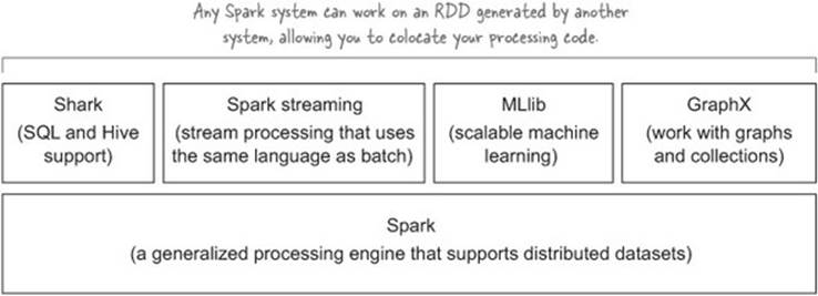
Spark consists of a core set of APIs and an execution engine, on top of which exist other Spark systems that provide APIs and processing capabilities for specialized activities, such as designing stream-processing pipelines. The core Spark systems are shown in figure 9.7.

Figure 9.7. Spark systems

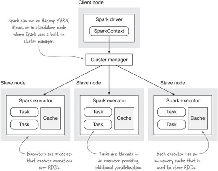
The Spark components can be seen in figure 9.8. The Spark driver is responsible for communicating with a cluster manager to execute operations and the Spark executors handle the actual operation execution and data management.

Figure 9.8. Spark architecture

Data in Spark is represented using RDDs (resilient distributed datasets), which are an abstraction over a collection of items. RDDs are distributed over a cluster so that each cluster node will store and manage a certain range of the items in an RDD. RDDs can be created from a number of sources, such as regular Scala collections or data from HDFS (synthesized via Hadoop input format classes). RDDs can be in-memory, on disk, or a mix of the two.^[¹¹^]

¹¹ More information on RDD caching and persistence can be found in the Spark Programming Guide at https://spark.apache.org/docs/latest/programming-guide.html#rdd-persistence.

The following example shows how an RDD can be created from a text file:

scala> val stocks = sc.textFile("stocks.txt")

stocks: org.apache.spark.rdd.RDD[String] = MappedRDD[122] at textFile

The Spark RDD class has various operations that you can perform on the RDD. RDD operations in Spark fall into two categories—transformations and actions:

· Transformations operate on an RDD to create a new RDD. Examples of transformation functions include map, flatMap, reduceByKey, and distinct.^[¹²^]

¹² A more complete list of transformations is shown in the Spark Programming Guide at https://spark.apache.org/docs/latest/programming-guide.html#transformations.

· Actions perform some activity over an RDD, after which they return results to the driver. For example, the collect function returns the entire RDD contents to the driver process, and the take function allows you to select the first N items in a dataset.^[¹³^]

¹³ A more complete list of actions can be found in the Spark Programming Guide at https://spark.apache.org/docs/latest/programming-guide.html#actions.

Lazy transformations

Spark will lazily evaluate transformations, so you actually need to execute an action for Spark to execute your operations.

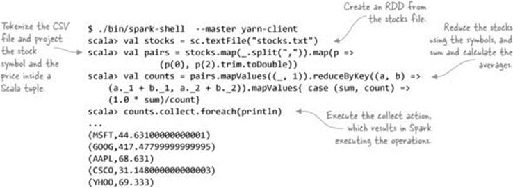
Let’s take a look at an example of a Spark application that calculates the average stock price for each symbol. To run the example, you’ll need to have Spark installed,^[¹⁴^] after which you can launch the shell:

¹⁴ To install and configure Spark on YARN, follow the instructions on “Running Spark on YARN” at http://spark.apache.org/docs/latest/running-on-yarn.html.

This was a very brief introduction to Spark—the Spark online documentation is excellent and is worth exploring to learn more about Spark.^[¹⁵^] Let’s now turn to an introduction to how Spark works with Hadoop.

¹⁵ A great starting place for learning about Spark is the Spark Programming Guide, http://spark.apache.org/docs/latest/programming-guide.html.

9.3.2. Spark on Hadoop

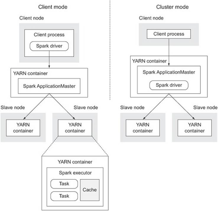
Spark supports several cluster managers, one of them being YARN. In this mode, the Spark executors are YARN containers, and the Spark ApplicationMaster is responsible for managing the Spark executors and sending them commands. The Spark driver is either contained within the client process or inside the ApplicationMaster, depending on whether you’re running in client mode or cluster mode:

· In client mode the driver resides inside the client, which means that executing a series of Spark tasks in this mode will be interrupted if the client process is terminated. This mode works well for the Spark shell, but it isn’t suitable for use when Spark is being used in a non-interactive method.

· In cluster mode the driver executes in the ApplicationMaster and doesn’t rely on the client to exist in order to execute tasks. This mode works best for cases where you have some existing Spark code that you wish to execute and that doesn’t require any interaction from you.

Figure 9.9 shows the architecture of Spark running on YARN.

Figure 9.9. Spark running on YARN

The default installation of Spark is set up for standalone mode, so you’ll have to configure Spark to make it work with YARN.^[¹⁶^] The Spark scripts and tools don’t change when you’re running on YARN, so once you’ve configured Spark to use YARN, you can run the Spark shell just like you did in the previous example.

¹⁶ Follow the instructions at https://spark.apache.org/docs/latest/running-on-yarn.html to set up Spark to use YARN.

Now that you understand some Spark basics and how it works on YARN, let’s look at how you can execute SQL using Spark.

9.3.3. SQL with Spark

This section covers Spark SQL, which is part of the core Spark system. Three areas of Spark SQL will be examined: executing SQL against your RDDs, using integrated query language features that provide a more expressive way to work with your data, and integrating HiveQL with Spark.

Stability of Spark SQL

Spark SQL is currently labeled as alpha quality, so it’s probably best not to use it in your production code until it’s marked as production-ready.

Technique 98 Calculating stock averages with Spark SQL

In this technique you’ll learn how to use Spark SQL to calculate the average price for each stock symbol.

Problem

You have a Spark processing pipeline, and expressing your functions would be simpler using SQL as opposed to the Spark APIs.

Solution

Discussion

The first step in this technique is to define a class that will represent each record in your Spark table. In this example, you’ll calculate the stock price averages, so all you need is a class with two fields to store the stock symbol and price:

scala> case class Stock(symbol: String, price: Double)

Why use Scala for Spark examples?

In this section we’ll use Scala to show Spark examples. The Scala API, until recently, has been much more concise than Spark’s Java API, although with the release of Spark 1.0, the Java support in Spark now uses lambdas to expose a less verbose API.

Next you need to register an RDD of these Stock objects as a table so that you can perform SQL operations on it. You can create a table from any Spark RDD. The following example shows how you can load the stocks data from HDFS and register it as a table:

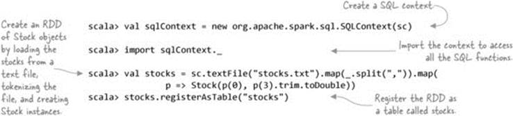
Now you’re ready to issue queries against the stocks table. The following shows how you’d calculate the average price for each symbol:

scala> val stock_averages = sql(

"SELECT symbol, AVG(price) FROM stocks GROUP BY symbol")

scala> stock_averages.collect().foreach(println)

[CSCO,31.564999999999998]

[GOOG,427.032]

[MSFT,45.281]

[AAPL,70.54599999999999]

[YHOO,73.29299999999999]

The sql function returns a SchemaRDD, which supports standard RDD operations. This is where the novel aspect of Spark SQL comes into play—mixing SQL and regular data processing paradigms together. You use SQL to create an RDD and you can then immediately turn around and execute your usual Spark transformations over that data.

In addition to supporting the standard Spark RDD operations, SchemaRDD also allows you to execute SQL-like functions such as where and join over the data, which is covered in the next technique.^[¹⁷^]

¹⁷ Language-integrated queries that allow more natural language expression of queries can be seen at the Scala docs for the SchemaRDD class at http://spark.apache.org/docs/latest/api/scala/index.html#org.apache.spark.sql.SchemaRDD.

Technique 99 Language-integrated queries

The previous technique demonstrated how you can execute SQL over your Spark data. Spark 1.0 also introduced a feature called language-integrated queries, which expose SQL constructs as functions, allowing you to craft code that’s not only fluent but that expresses operations using natural language constructs. In this technique you’ll see how to use these functions on your RDDs.

Problem

Although the Spark RDD functions are expressive, they don’t yield code that is particularly human-readable.

Solution

Use Spark’s language-integrated queries.

Discussion

Once again, let’s try to calculate the average stock prices, this time using language-integrated queries. This example uses the groupBy function to calculate the average stock price:

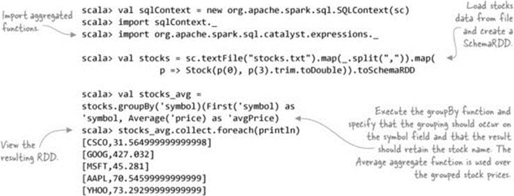
The preceding code leverages the Average and First aggregate functions—there are other aggregate functions such as Count, Min, and Max, among others.^[¹⁸^]

¹⁸ See the code at the following link for the complete list: https://github.com/apache/spark/blob/master/sql/catalyst/src/main/scala/org/apache/spark/sql/catalyst/expressions/aggregates.scala.

The next is more straightforward; it simply selects all the quotes for days where the value was over $100:

scala> stocks.where('price >= 100).collect.foreach(println)

[AAPL,200.26]

[AAPL,112.5]

...

The third option with Spark SQL is to use HiveQL, which is useful when you want to execute more complex SQL grammar.

Technique 100 Hive and Spark SQL

You can also work with data in Hive tables in Spark. This technique examines how you can execute a query against a Hive table.

Problem

You want to work with Hive data in Spark.

Solution

Use Spark’s HiveContext to issue HiveQL statements and work with the results in Spark.

Discussion

Earlier in this chapter you created a stocks table in Hive (in technique 89). Let’s query that stocks table using HiveQL from within Spark and then perform some additional manipulations within Spark:

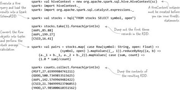
You have access to the complete HiveQL grammar in Spark, as the commands that are wrapped inside the hql calls are sent directly to Hive. You can load tables, insert into tables, and perform any Hive command that’s needed, all directly from Spark. Spark’s Hive integration also includes support for using Hive UDFs, UDAFs, and UDTFs in your queries.

This completes our brief look at Spark SQL.

9.4. Chapter summary

SQL access to data in Hadoop is essential for organizations, as not all users who want to interact with data are programmers. SQL is often the lingua franca for not only data analysts but also for data scientists and nontechnical members of your organization.

In this chapter I introduced three tools that can be used to work with your data via SQL. Hive has been around the longest and is currently the most full-featured SQL engine you can use. Impala is worth a serious look if Hive is not providing a rapid enough level of interaction with your data. And finally, Spark SQL provides a glimpse into the future, where technical members of your organization such as programmers and data scientists can fuse together SQL and Scala to build complex and efficient processing pipelines.