Hadoop: The Definitive Guide (2015)
Part I. Hadoop Fundamentals
Chapter 2. MapReduce
MapReduce is a programming model for data processing. The model is simple, yet not too simple to express useful programs in. Hadoop can run MapReduce programs written in various languages; in this chapter, we look at the same program expressed in Java, Ruby, and Python. Most importantly, MapReduce programs are inherently parallel, thus putting very large-scale data analysis into the hands of anyone with enough machines at their disposal. MapReduce comes into its own for large datasets, so let’s start by looking at one.
A Weather Dataset
For our example, we will write a program that mines weather data. Weather sensors collect data every hour at many locations across the globe and gather a large volume of log data, which is a good candidate for analysis with MapReduce because we want to process all the data, and the data is semi-structured and record-oriented.
Data Format
The data we will use is from the National Climatic Data Center, or NCDC. The data is stored using a line-oriented ASCII format, in which each line is a record. The format supports a rich set of meteorological elements, many of which are optional or with variable data lengths. For simplicity, we focus on the basic elements, such as temperature, which are always present and are of fixed width.
Example 2-1 shows a sample line with some of the salient fields annotated. The line has been split into multiple lines to show each field; in the real file, fields are packed into one line with no delimiters.
Example 2-1. Format of a National Climatic Data Center record
0057
332130 # USAF weather station identifier
99999 # WBAN weather station identifier
19500101 # observation date
0300 # observation time
4
+51317 # latitude (degrees x 1000)
+028783 # longitude (degrees x 1000)
FM-12
+0171 # elevation (meters)
99999
V020
320 # wind direction (degrees)
1 # quality code
N
0072
1
00450 # sky ceiling height (meters)
1 # quality code
C
N
010000 # visibility distance (meters)
1 # quality code
N
9
-0128 # air temperature (degrees Celsius x 10)
1 # quality code
-0139 # dew point temperature (degrees Celsius x 10)
1 # quality code
10268 # atmospheric pressure (hectopascals x 10)
1 # quality code
Datafiles are organized by date and weather station. There is a directory for each year from 1901 to 2001, each containing a gzipped file for each weather station with its readings for that year. For example, here are the first entries for 1990:
% ls raw/1990 | head
010010-99999-1990.gz
010014-99999-1990.gz
010015-99999-1990.gz
010016-99999-1990.gz
010017-99999-1990.gz
010030-99999-1990.gz
010040-99999-1990.gz
010080-99999-1990.gz
010100-99999-1990.gz
010150-99999-1990.gz
There are tens of thousands of weather stations, so the whole dataset is made up of a large number of relatively small files. It’s generally easier and more efficient to process a smaller number of relatively large files, so the data was preprocessed so that each year’s readings were concatenated into a single file. (The means by which this was carried out is described in Appendix C.)
Analyzing the Data with Unix Tools
What’s the highest recorded global temperature for each year in the dataset? We will answer this first without using Hadoop, as this information will provide a performance baseline and a useful means to check our results.
The classic tool for processing line-oriented data is awk. Example 2-2 is a small script to calculate the maximum temperature for each year.
Example 2-2. A program for finding the maximum recorded temperature by year from NCDC weather records
#!/usr/bin/env bash
for year in all/*
do
echo -ne `basename $year .gz`"\t"
gunzip -c $year | \
awk '{ temp = substr($0, 88, 5) + 0;
q = substr($0, 93, 1);
if (temp !=9999 && q ~ /[01459]/ && temp > max) max = temp }
END { print max }'
done
The script loops through the compressed year files, first printing the year, and then processing each file using awk. The awk script extracts two fields from the data: the air temperature and the quality code. The air temperature value is turned into an integer by adding 0. Next, a test is applied to see whether the temperature is valid (the value 9999 signifies a missing value in the NCDC dataset) and whether the quality code indicates that the reading is not suspect or erroneous. If the reading is OK, the value is compared with the maximum value seen so far, which is updated if a new maximum is found. The END block is executed after all the lines in the file have been processed, and it prints the maximum value.
Here is the beginning of a run:
% ./max_temperature.sh
1901 317
1902 244
1903 289
1904 256
1905 283
...
The temperature values in the source file are scaled by a factor of 10, so this works out as a maximum temperature of 31.7°C for 1901 (there were very few readings at the beginning of the century, so this is plausible). The complete run for the century took 42 minutes in one run on a single EC2 High-CPU Extra Large instance.
To speed up the processing, we need to run parts of the program in parallel. In theory, this is straightforward: we could process different years in different processes, using all the available hardware threads on a machine. There are a few problems with this, however.
First, dividing the work into equal-size pieces isn’t always easy or obvious. In this case, the file size for different years varies widely, so some processes will finish much earlier than others. Even if they pick up further work, the whole run is dominated by the longest file. A better approach, although one that requires more work, is to split the input into fixed-size chunks and assign each chunk to a process.
Second, combining the results from independent processes may require further processing. In this case, the result for each year is independent of other years, and they may be combined by concatenating all the results and sorting by year. If using the fixed-size chunk approach, the combination is more delicate. For this example, data for a particular year will typically be split into several chunks, each processed independently. We’ll end up with the maximum temperature for each chunk, so the final step is to look for the highest of these maximums for each year.
Third, you are still limited by the processing capacity of a single machine. If the best time you can achieve is 20 minutes with the number of processors you have, then that’s it. You can’t make it go faster. Also, some datasets grow beyond the capacity of a single machine. When we start using multiple machines, a whole host of other factors come into play, mainly falling into the categories of coordination and reliability. Who runs the overall job? How do we deal with failed processes?
So, although it’s feasible to parallelize the processing, in practice it’s messy. Using a framework like Hadoop to take care of these issues is a great help.
Analyzing the Data with Hadoop
To take advantage of the parallel processing that Hadoop provides, we need to express our query as a MapReduce job. After some local, small-scale testing, we will be able to run it on a cluster of machines.
Map and Reduce
MapReduce works by breaking the processing into two phases: the map phase and the reduce phase. Each phase has key-value pairs as input and output, the types of which may be chosen by the programmer. The programmer also specifies two functions: the map function and the reduce function.
The input to our map phase is the raw NCDC data. We choose a text input format that gives us each line in the dataset as a text value. The key is the offset of the beginning of the line from the beginning of the file, but as we have no need for this, we ignore it.
Our map function is simple. We pull out the year and the air temperature, because these are the only fields we are interested in. In this case, the map function is just a data preparation phase, setting up the data in such a way that the reduce function can do its work on it: finding the maximum temperature for each year. The map function is also a good place to drop bad records: here we filter out temperatures that are missing, suspect, or erroneous.
To visualize the way the map works, consider the following sample lines of input data (some unused columns have been dropped to fit the page, indicated by ellipses):
0067011990999991950051507004...9999999N9+00001+99999999999...
0043011990999991950051512004...9999999N9+00221+99999999999...
0043011990999991950051518004...9999999N9-00111+99999999999...
0043012650999991949032412004...0500001N9+01111+99999999999...
0043012650999991949032418004...0500001N9+00781+99999999999...
These lines are presented to the map function as the key-value pairs:
(0, 0067011990999991950051507004...9999999N9+00001+99999999999...)
(106, 0043011990999991950051512004...9999999N9+00221+99999999999...)
(212, 0043011990999991950051518004...9999999N9-00111+99999999999...)
(318, 0043012650999991949032412004...0500001N9+01111+99999999999...)
(424, 0043012650999991949032418004...0500001N9+00781+99999999999...)
The keys are the line offsets within the file, which we ignore in our map function. The map function merely extracts the year and the air temperature (indicated in bold text), and emits them as its output (the temperature values have been interpreted as integers):
(1950, 0)
(1950, 22)
(1950, −11)
(1949, 111)
(1949, 78)
The output from the map function is processed by the MapReduce framework before being sent to the reduce function. This processing sorts and groups the key-value pairs by key. So, continuing the example, our reduce function sees the following input:
(1949, [111, 78])
(1950, [0, 22, −11])
Each year appears with a list of all its air temperature readings. All the reduce function has to do now is iterate through the list and pick up the maximum reading:
(1949, 111)
(1950, 22)
This is the final output: the maximum global temperature recorded in each year.
The whole data flow is illustrated in Figure 2-1. At the bottom of the diagram is a Unix pipeline, which mimics the whole MapReduce flow and which we will see again later in this chapter when we look at Hadoop Streaming.
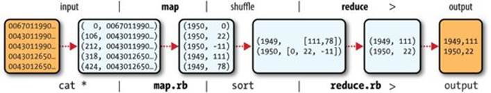
Figure 2-1. MapReduce logical data flow
Java MapReduce
Having run through how the MapReduce program works, the next step is to express it in code. We need three things: a map function, a reduce function, and some code to run the job. The map function is represented by the Mapper class, which declares an abstract map() method.Example 2-3 shows the implementation of our map function.
Example 2-3. Mapper for the maximum temperature example
import java.io.IOException;
import org.apache.hadoop.io.IntWritable;
import org.apache.hadoop.io.LongWritable;
import org.apache.hadoop.io.Text;
import org.apache.hadoop.mapreduce.Mapper;
public class MaxTemperatureMapper
extends Mapper<LongWritable, Text, Text, IntWritable> {
private static final int MISSING = 9999;
@Override
public void map(LongWritable key, Text value, Context context)
throws IOException, InterruptedException {
String line = value.toString();
String year = line.substring(15, 19);
int airTemperature;
if (line.charAt(87) == '+') { // parseInt doesn't like leading plus signs
airTemperature = Integer.parseInt(line.substring(88, 92));
} else {
airTemperature = Integer.parseInt(line.substring(87, 92));
}
String quality = line.substring(92, 93);
if (airTemperature != MISSING && quality.matches("[01459]")) {
context.write(new Text(year), new IntWritable(airTemperature));
}
}
}
The Mapper class is a generic type, with four formal type parameters that specify the input key, input value, output key, and output value types of the map function. For the present example, the input key is a long integer offset, the input value is a line of text, the output key is a year, and the output value is an air temperature (an integer). Rather than using built-in Java types, Hadoop provides its own set of basic types that are optimized for network serialization. These are found in the org.apache.hadoop.io package. Here we use LongWritable, which corresponds to a Java Long, Text (like Java String), and IntWritable (like Java Integer).
The map() method is passed a key and a value. We convert the Text value containing the line of input into a Java String, then use its substring() method to extract the columns we are interested in.
The map() method also provides an instance of Context to write the output to. In this case, we write the year as a Text object (since we are just using it as a key), and the temperature is wrapped in an IntWritable. We write an output record only if the temperature is present and the quality code indicates the temperature reading is OK.
The reduce function is similarly defined using a Reducer, as illustrated in Example 2-4.
Example 2-4. Reducer for the maximum temperature example
import java.io.IOException;
import org.apache.hadoop.io.IntWritable;
import org.apache.hadoop.io.Text;
import org.apache.hadoop.mapreduce.Reducer;
public class MaxTemperatureReducer
extends Reducer<Text, IntWritable, Text, IntWritable> {
@Override
public void reduce(Text key, Iterable<IntWritable> values, Context context)
throws IOException, InterruptedException {
int maxValue = Integer.MIN_VALUE;
for (IntWritable value : values) {
maxValue = Math.max(maxValue, value.get());
}
context.write(key, new IntWritable(maxValue));
}
}
Again, four formal type parameters are used to specify the input and output types, this time for the reduce function. The input types of the reduce function must match the output types of the map function: Text and IntWritable. And in this case, the output types of the reduce function are Text and IntWritable, for a year and its maximum temperature, which we find by iterating through the temperatures and comparing each with a record of the highest found so far.
The third piece of code runs the MapReduce job (see Example 2-5).
Example 2-5. Application to find the maximum temperature in the weather dataset
import org.apache.hadoop.fs.Path;
import org.apache.hadoop.io.IntWritable;
import org.apache.hadoop.io.Text;
import org.apache.hadoop.mapreduce.Job;
import org.apache.hadoop.mapreduce.lib.input.FileInputFormat;
import org.apache.hadoop.mapreduce.lib.output.FileOutputFormat;
public class MaxTemperature {
public static void main(String[] args) throws Exception {
if (args.length != 2) {
System.err.println("Usage: MaxTemperature <input path> <output path>");
System.exit(-1);
}
Job job = new Job();
job.setJarByClass(MaxTemperature.class);
job.setJobName("Max temperature");
FileInputFormat.addInputPath(job, new Path(args[0]));
FileOutputFormat.setOutputPath(job, new Path(args[1]));
job.setMapperClass(MaxTemperatureMapper.class);
job.setReducerClass(MaxTemperatureReducer.class);
job.setOutputKeyClass(Text.class);
job.setOutputValueClass(IntWritable.class);
System.exit(job.waitForCompletion(true) ? 0 : 1);
}
}
A Job object forms the specification of the job and gives you control over how the job is run. When we run this job on a Hadoop cluster, we will package the code into a JAR file (which Hadoop will distribute around the cluster). Rather than explicitly specifying the name of the JAR file, we can pass a class in the Job’s setJarByClass() method, which Hadoop will use to locate the relevant JAR file by looking for the JAR file containing this class.
Having constructed a Job object, we specify the input and output paths. An input path is specified by calling the static addInputPath() method on FileInputFormat, and it can be a single file, a directory (in which case, the input forms all the files in that directory), or a file pattern. As the name suggests, addInputPath() can be called more than once to use input from multiple paths.
The output path (of which there is only one) is specified by the static setOutputPath() method on FileOutputFormat. It specifies a directory where the output files from the reduce function are written. The directory shouldn’t exist before running the job because Hadoop will complain and not run the job. This precaution is to prevent data loss (it can be very annoying to accidentally overwrite the output of a long job with that of another).
Next, we specify the map and reduce types to use via the setMapperClass() and setReducerClass() methods.
The setOutputKeyClass() and setOutputValueClass() methods control the output types for the reduce function, and must match what the Reduce class produces. The map output types default to the same types, so they do not need to be set if the mapper produces the same types as the reducer (as it does in our case). However, if they are different, the map output types must be set using the setMapOutputKeyClass() and setMapOutputValueClass() methods.
The input types are controlled via the input format, which we have not explicitly set because we are using the default TextInputFormat.
After setting the classes that define the map and reduce functions, we are ready to run the job. The waitForCompletion() method on Job submits the job and waits for it to finish. The single argument to the method is a flag indicating whether verbose output is generated. When true, the job writes information about its progress to the console.
The return value of the waitForCompletion() method is a Boolean indicating success (true) or failure (false), which we translate into the program’s exit code of 0 or 1.
NOTE
The Java MapReduce API used in this section, and throughout the book, is called the “new API”; it replaces the older, functionally equivalent API. The differences between the two APIs are explained in Appendix D, along with tips on how to convert between the two APIs. You can also find the old API equivalent of the maximum temperature application there.
A test run
After writing a MapReduce job, it’s normal to try it out on a small dataset to flush out any immediate problems with the code. First, install Hadoop in standalone mode (there are instructions for how to do this in Appendix A). This is the mode in which Hadoop runs using the local filesystem with a local job runner. Then, install and compile the examples using the instructions on the book’s website.
Let’s test it on the five-line sample discussed earlier (the output has been slightly reformatted to fit the page, and some lines have been removed):
% export HADOOP_CLASSPATH=hadoop-examples.jar
% hadoop MaxTemperature input/ncdc/sample.txt output
14/09/16 09:48:39 WARN util.NativeCodeLoader: Unable to load native-hadoop
library for your platform... using builtin-java classes where applicable
14/09/16 09:48:40 WARN mapreduce.JobSubmitter: Hadoop command-line option
parsing not performed. Implement the Tool interface and execute your application
with ToolRunner to remedy this.
14/09/16 09:48:40 INFO input.FileInputFormat: Total input paths to process : 1
14/09/16 09:48:40 INFO mapreduce.JobSubmitter: number of splits:1
14/09/16 09:48:40 INFO mapreduce.JobSubmitter: Submitting tokens for job:
job_local26392882_0001
14/09/16 09:48:40 INFO mapreduce.Job: The url to track the job:
http://localhost:8080/
14/09/16 09:48:40 INFO mapreduce.Job: Running job: job_local26392882_0001
14/09/16 09:48:40 INFO mapred.LocalJobRunner: OutputCommitter set in config null
14/09/16 09:48:40 INFO mapred.LocalJobRunner: OutputCommitter is
org.apache.hadoop.mapreduce.lib.output.FileOutputCommitter
14/09/16 09:48:40 INFO mapred.LocalJobRunner: Waiting for map tasks
14/09/16 09:48:40 INFO mapred.LocalJobRunner: Starting task:
attempt_local26392882_0001_m_000000_0
14/09/16 09:48:40 INFO mapred.Task: Using ResourceCalculatorProcessTree : null
14/09/16 09:48:40 INFO mapred.LocalJobRunner:
14/09/16 09:48:40 INFO mapred.Task: Task:attempt_local26392882_0001_m_000000_0
is done. And is in the process of committing
14/09/16 09:48:40 INFO mapred.LocalJobRunner: map
14/09/16 09:48:40 INFO mapred.Task: Task 'attempt_local26392882_0001_m_000000_0'
done.
14/09/16 09:48:40 INFO mapred.LocalJobRunner: Finishing task:
attempt_local26392882_0001_m_000000_0
14/09/16 09:48:40 INFO mapred.LocalJobRunner: map task executor complete.
14/09/16 09:48:40 INFO mapred.LocalJobRunner: Waiting for reduce tasks
14/09/16 09:48:40 INFO mapred.LocalJobRunner: Starting task:
attempt_local26392882_0001_r_000000_0
14/09/16 09:48:40 INFO mapred.Task: Using ResourceCalculatorProcessTree : null
14/09/16 09:48:40 INFO mapred.LocalJobRunner: 1 / 1 copied.
14/09/16 09:48:40 INFO mapred.Merger: Merging 1 sorted segments
14/09/16 09:48:40 INFO mapred.Merger: Down to the last merge-pass, with 1
segments left of total size: 50 bytes
14/09/16 09:48:40 INFO mapred.Merger: Merging 1 sorted segments
14/09/16 09:48:40 INFO mapred.Merger: Down to the last merge-pass, with 1
segments left of total size: 50 bytes
14/09/16 09:48:40 INFO mapred.LocalJobRunner: 1 / 1 copied.
14/09/16 09:48:40 INFO mapred.Task: Task:attempt_local26392882_0001_r_000000_0
is done. And is in the process of committing
14/09/16 09:48:40 INFO mapred.LocalJobRunner: 1 / 1 copied.
14/09/16 09:48:40 INFO mapred.Task: Task attempt_local26392882_0001_r_000000_0
is allowed to commit now
14/09/16 09:48:40 INFO output.FileOutputCommitter: Saved output of task
'attempt...local26392882_0001_r_000000_0' to file:/Users/tom/book-workspace/
hadoop-book/output/_temporary/0/task_local26392882_0001_r_000000
14/09/16 09:48:40 INFO mapred.LocalJobRunner: reduce > reduce
14/09/16 09:48:40 INFO mapred.Task: Task 'attempt_local26392882_0001_r_000000_0'
done.
14/09/16 09:48:40 INFO mapred.LocalJobRunner: Finishing task:
attempt_local26392882_0001_r_000000_0
14/09/16 09:48:40 INFO mapred.LocalJobRunner: reduce task executor complete.
14/09/16 09:48:41 INFO mapreduce.Job: Job job_local26392882_0001 running in uber
mode : false
14/09/16 09:48:41 INFO mapreduce.Job: map 100% reduce 100%
14/09/16 09:48:41 INFO mapreduce.Job: Job job_local26392882_0001 completed
successfully
14/09/16 09:48:41 INFO mapreduce.Job: Counters: 30
File System Counters
FILE: Number of bytes read=377168
FILE: Number of bytes written=828464
FILE: Number of read operations=0
FILE: Number of large read operations=0
FILE: Number of write operations=0
Map-Reduce Framework
Map input records=5
Map output records=5
Map output bytes=45
Map output materialized bytes=61
Input split bytes=129
Combine input records=0
Combine output records=0
Reduce input groups=2
Reduce shuffle bytes=61
Reduce input records=5
Reduce output records=2
Spilled Records=10
Shuffled Maps =1
Failed Shuffles=0
Merged Map outputs=1
GC time elapsed (ms)=39
Total committed heap usage (bytes)=226754560
File Input Format Counters
Bytes Read=529
File Output Format Counters
Bytes Written=29
When the hadoop command is invoked with a classname as the first argument, it launches a Java virtual machine (JVM) to run the class. The hadoop command adds the Hadoop libraries (and their dependencies) to the classpath and picks up the Hadoop configuration, too. To add the application classes to the classpath, we’ve defined an environment variable called HADOOP_CLASSPATH, which the hadoop script picks up.
NOTE
When running in local (standalone) mode, the programs in this book all assume that you have set the HADOOP_CLASSPATH in this way. The commands should be run from the directory that the example code is installed in.
The output from running the job provides some useful information. For example, we can see that the job was given an ID of job_local26392882_0001, and it ran one map task and one reduce task (with the following IDs: attempt_local26392882_0001_m_000000_0 andattempt_local26392882_0001_r_000000_0). Knowing the job and task IDs can be very useful when debugging MapReduce jobs.
The last section of the output, titled “Counters,” shows the statistics that Hadoop generates for each job it runs. These are very useful for checking whether the amount of data processed is what you expected. For example, we can follow the number of records that went through the system: five map input records produced five map output records (since the mapper emitted one output record for each valid input record), then five reduce input records in two groups (one for each unique key) produced two reduce output records.
The output was written to the output directory, which contains one output file per reducer. The job had a single reducer, so we find a single file, named part-r-00000:
% cat output/part-r-00000
1949 111
1950 22
This result is the same as when we went through it by hand earlier. We interpret this as saying that the maximum temperature recorded in 1949 was 11.1°C, and in 1950 it was 2.2°C.
Scaling Out
You’ve seen how MapReduce works for small inputs; now it’s time to take a bird’s-eye view of the system and look at the data flow for large inputs. For simplicity, the examples so far have used files on the local filesystem. However, to scale out, we need to store the data in a distributed filesystem (typically HDFS, which you’ll learn about in the next chapter). This allows Hadoop to move the MapReduce computation to each machine hosting a part of the data, using Hadoop’s resource management system, called YARN (see Chapter 4). Let’s see how this works.
Data Flow
First, some terminology. A MapReduce job is a unit of work that the client wants to be performed: it consists of the input data, the MapReduce program, and configuration information. Hadoop runs the job by dividing it into tasks, of which there are two types: map tasks and reduce tasks. The tasks are scheduled using YARN and run on nodes in the cluster. If a task fails, it will be automatically rescheduled to run on a different node.
Hadoop divides the input to a MapReduce job into fixed-size pieces called input splits, or just splits. Hadoop creates one map task for each split, which runs the user-defined map function for each record in the split.
Having many splits means the time taken to process each split is small compared to the time to process the whole input. So if we are processing the splits in parallel, the processing is better load balanced when the splits are small, since a faster machine will be able to process proportionally more splits over the course of the job than a slower machine. Even if the machines are identical, failed processes or other jobs running concurrently make load balancing desirable, and the quality of the load balancing increases as the splits become more fine grained.
On the other hand, if splits are too small, the overhead of managing the splits and map task creation begins to dominate the total job execution time. For most jobs, a good split size tends to be the size of an HDFS block, which is 128 MB by default, although this can be changed for the cluster (for all newly created files) or specified when each file is created.
Hadoop does its best to run the map task on a node where the input data resides in HDFS, because it doesn’t use valuable cluster bandwidth. This is called the data locality optimization. Sometimes, however, all the nodes hosting the HDFS block replicas for a map task’s input split are running other map tasks, so the job scheduler will look for a free map slot on a node in the same rack as one of the blocks. Very occasionally even this is not possible, so an off-rack node is used, which results in an inter-rack network transfer. The three possibilities are illustrated inFigure 2-2.
It should now be clear why the optimal split size is the same as the block size: it is the largest size of input that can be guaranteed to be stored on a single node. If the split spanned two blocks, it would be unlikely that any HDFS node stored both blocks, so some of the split would have to be transferred across the network to the node running the map task, which is clearly less efficient than running the whole map task using local data.
Map tasks write their output to the local disk, not to HDFS. Why is this? Map output is intermediate output: it’s processed by reduce tasks to produce the final output, and once the job is complete, the map output can be thrown away. So, storing it in HDFS with replication would be overkill. If the node running the map task fails before the map output has been consumed by the reduce task, then Hadoop will automatically rerun the map task on another node to re-create the map output.
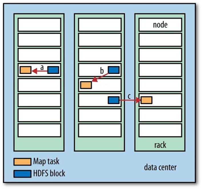
Figure 2-2. Data-local (a), rack-local (b), and off-rack (c) map tasks
Reduce tasks don’t have the advantage of data locality; the input to a single reduce task is normally the output from all mappers. In the present example, we have a single reduce task that is fed by all of the map tasks. Therefore, the sorted map outputs have to be transferred across the network to the node where the reduce task is running, where they are merged and then passed to the user-defined reduce function. The output of the reduce is normally stored in HDFS for reliability. As explained in Chapter 3, for each HDFS block of the reduce output, the first replica is stored on the local node, with other replicas being stored on off-rack nodes for reliability. Thus, writing the reduce output does consume network bandwidth, but only as much as a normal HDFS write pipeline consumes.
The whole data flow with a single reduce task is illustrated in Figure 2-3. The dotted boxes indicate nodes, the dotted arrows show data transfers on a node, and the solid arrows show data transfers between nodes.
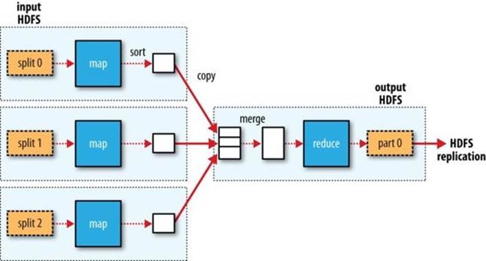
Figure 2-3. MapReduce data flow with a single reduce task
The number of reduce tasks is not governed by the size of the input, but instead is specified independently. In The Default MapReduce Job, you will see how to choose the number of reduce tasks for a given job.
When there are multiple reducers, the map tasks partition their output, each creating one partition for each reduce task. There can be many keys (and their associated values) in each partition, but the records for any given key are all in a single partition. The partitioning can be controlled by a user-defined partitioning function, but normally the default partitioner — which buckets keys using a hash function — works very well.
The data flow for the general case of multiple reduce tasks is illustrated in Figure 2-4. This diagram makes it clear why the data flow between map and reduce tasks is colloquially known as “the shuffle,” as each reduce task is fed by many map tasks. The shuffle is more complicated than this diagram suggests, and tuning it can have a big impact on job execution time, as you will see in Shuffle and Sort.
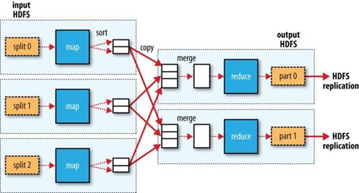
Figure 2-4. MapReduce data flow with multiple reduce tasks
Finally, it’s also possible to have zero reduce tasks. This can be appropriate when you don’t need the shuffle because the processing can be carried out entirely in parallel (a few examples are discussed in NLineInputFormat). In this case, the only off-node data transfer is when the map tasks write to HDFS (see Figure 2-5).
Combiner Functions
Many MapReduce jobs are limited by the bandwidth available on the cluster, so it pays to minimize the data transferred between map and reduce tasks. Hadoop allows the user to specify a combiner function to be run on the map output, and the combiner function’s output forms the input to the reduce function. Because the combiner function is an optimization, Hadoop does not provide a guarantee of how many times it will call it for a particular map output record, if at all. In other words, calling the combiner function zero, one, or many times should produce the same output from the reducer.
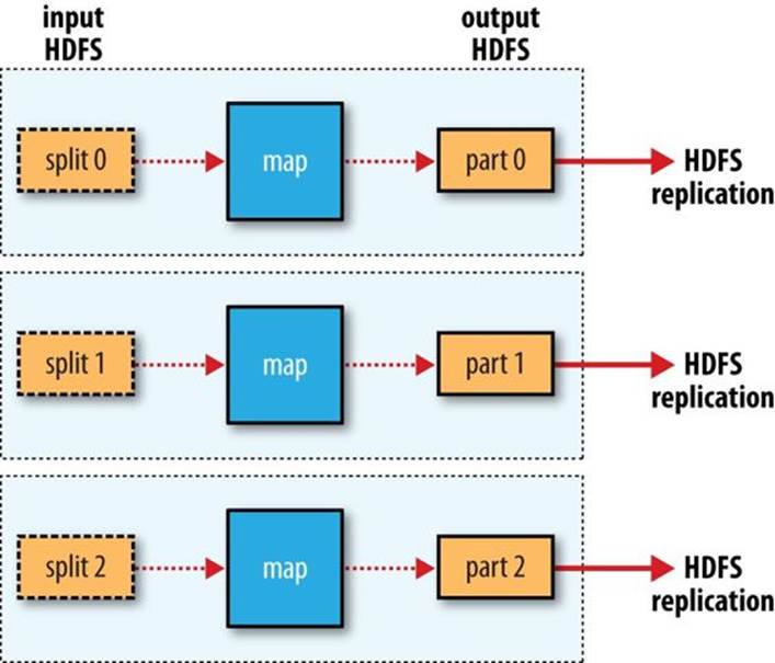
Figure 2-5. MapReduce data flow with no reduce tasks
The contract for the combiner function constrains the type of function that may be used. This is best illustrated with an example. Suppose that for the maximum temperature example, readings for the year 1950 were processed by two maps (because they were in different splits). Imagine the first map produced the output:
(1950, 0)
(1950, 20)
(1950, 10)
and the second produced:
(1950, 25)
(1950, 15)
The reduce function would be called with a list of all the values:
(1950, [0, 20, 10, 25, 15])
with output:
(1950, 25)
since 25 is the maximum value in the list. We could use a combiner function that, just like the reduce function, finds the maximum temperature for each map output. The reduce function would then be called with:
(1950, [20, 25])
and would produce the same output as before. More succinctly, we may express the function calls on the temperature values in this case as follows:
max(0, 20, 10, 25, 15) = max(max(0, 20, 10), max(25, 15)) = max(20, 25) = 25
Not all functions possess this property.[20] For example, if we were calculating mean temperatures, we couldn’t use the mean as our combiner function, because:
mean(0, 20, 10, 25, 15) = 14
but:
mean(mean(0, 20, 10), mean(25, 15)) = mean(10, 20) = 15
The combiner function doesn’t replace the reduce function. (How could it? The reduce function is still needed to process records with the same key from different maps.) But it can help cut down the amount of data shuffled between the mappers and the reducers, and for this reason alone it is always worth considering whether you can use a combiner function in your MapReduce job.
Specifying a combiner function
Going back to the Java MapReduce program, the combiner function is defined using the Reducer class, and for this application, it is the same implementation as the reduce function in MaxTemperatureReducer. The only change we need to make is to set the combiner class on the Job (seeExample 2-6).
Example 2-6. Application to find the maximum temperature, using a combiner function for efficiency
public class MaxTemperatureWithCombiner {
public static void main(String[] args) throws Exception {
if (args.length != 2) {
System.err.println("Usage: MaxTemperatureWithCombiner <input path> " +
"<output path>");
System.exit(-1);
}
Job job = new Job();
job.setJarByClass(MaxTemperatureWithCombiner.class);
job.setJobName("Max temperature");
FileInputFormat.addInputPath(job, new Path(args[0]));
FileOutputFormat.setOutputPath(job, new Path(args[1]));
job.setMapperClass(MaxTemperatureMapper.class);
job.setCombinerClass(MaxTemperatureReducer.class);
job.setReducerClass(MaxTemperatureReducer.class);
job.setOutputKeyClass(Text.class);
job.setOutputValueClass(IntWritable.class);
System.exit(job.waitForCompletion(true) ? 0 : 1);
}
}
Running a Distributed MapReduce Job
The same program will run, without alteration, on a full dataset. This is the point of MapReduce: it scales to the size of your data and the size of your hardware. Here’s one data point: on a 10-node EC2 cluster running High-CPU Extra Large instances, the program took six minutes to run.[21]
We’ll go through the mechanics of running programs on a cluster in Chapter 6.
Hadoop Streaming
Hadoop provides an API to MapReduce that allows you to write your map and reduce functions in languages other than Java. Hadoop Streaming uses Unix standard streams as the interface between Hadoop and your program, so you can use any language that can read standard input and write to standard output to write your MapReduce program.[22]
Streaming is naturally suited for text processing. Map input data is passed over standard input to your map function, which processes it line by line and writes lines to standard output. A map output key-value pair is written as a single tab-delimited line. Input to the reduce function is in the same format — a tab-separated key-value pair — passed over standard input. The reduce function reads lines from standard input, which the framework guarantees are sorted by key, and writes its results to standard output.
Let’s illustrate this by rewriting our MapReduce program for finding maximum temperatures by year in Streaming.
Ruby
The map function can be expressed in Ruby as shown in Example 2-7.
Example 2-7. Map function for maximum temperature in Ruby
#!/usr/bin/env ruby
STDIN.each_line do |line|
val = line
year, temp, q = val[15,4], val[87,5], val[92,1]
puts "#{year}\t#{temp}" if (temp != "+9999" && q =~ /[01459]/)
end
The program iterates over lines from standard input by executing a block for each line from STDIN (a global constant of type IO). The block pulls out the relevant fields from each input line and, if the temperature is valid, writes the year and the temperature separated by a tab character,\t, to standard output (using puts).
NOTE
It’s worth drawing out a design difference between Streaming and the Java MapReduce API. The Java API is geared toward processing your map function one record at a time. The framework calls the map() method on your Mapper for each record in the input, whereas with Streaming the map program can decide how to process the input — for example, it could easily read and process multiple lines at a time since it’s in control of the reading. The user’s Java map implementation is “pushed” records, but it’s still possible to consider multiple lines at a time by accumulating previous lines in an instance variable in the Mapper.[23] In this case, you need to implement the close() method so that you know when the last record has been read, so you can finish processing the last group of lines.
Because the script just operates on standard input and output, it’s trivial to test the script without using Hadoop, simply by using Unix pipes:
% cat input/ncdc/sample.txt | ch02-mr-intro/src/main/ruby/max_temperature_map.rb
1950 +0000
1950 +0022
1950 -0011
1949 +0111
1949 +0078
The reduce function shown in Example 2-8 is a little more complex.
Example 2-8. Reduce function for maximum temperature in Ruby
#!/usr/bin/env ruby
last_key, max_val = nil, -1000000
STDIN.each_line do |line|
key, val = line.split("\t")
if last_key && last_key != key
puts "#{last_key}\t#{max_val}"
last_key, max_val = key, val.to_i
else
last_key, max_val = key, [max_val, val.to_i].max
end
end
puts "#{last_key}\t#{max_val}" if last_key
Again, the program iterates over lines from standard input, but this time we have to store some state as we process each key group. In this case, the keys are the years, and we store the last key seen and the maximum temperature seen so far for that key. The MapReduce framework ensures that the keys are ordered, so we know that if a key is different from the previous one, we have moved into a new key group. In contrast to the Java API, where you are provided an iterator over each key group, in Streaming you have to find key group boundaries in your program.
For each line, we pull out the key and value. Then, if we’ve just finished a group (last_key && last_key != key), we write the key and the maximum temperature for that group, separated by a tab character, before resetting the maximum temperature for the new key. If we haven’t just finished a group, we just update the maximum temperature for the current key.
The last line of the program ensures that a line is written for the last key group in the input.
We can now simulate the whole MapReduce pipeline with a Unix pipeline (which is equivalent to the Unix pipeline shown in Figure 2-1):
% cat input/ncdc/sample.txt | \
ch02-mr-intro/src/main/ruby/max_temperature_map.rb | \
sort | ch02-mr-intro/src/main/ruby/max_temperature_reduce.rb
1949 111
1950 22
The output is the same as that of the Java program, so the next step is to run it using Hadoop itself.
The hadoop command doesn’t support a Streaming option; instead, you specify the Streaming JAR file along with the jar option. Options to the Streaming program specify the input and output paths and the map and reduce scripts. This is what it looks like:
% hadoop jar $HADOOP_HOME/share/hadoop/tools/lib/hadoop-streaming-*.jar \
-input input/ncdc/sample.txt \
-output output \
-mapper ch02-mr-intro/src/main/ruby/max_temperature_map.rb \
-reducer ch02-mr-intro/src/main/ruby/max_temperature_reduce.rb
When running on a large dataset on a cluster, we should use the -combiner option to set the combiner:
% hadoop jar $HADOOP_HOME/share/hadoop/tools/lib/hadoop-streaming-*.jar \
-files ch02-mr-intro/src/main/ruby/max_temperature_map.rb,\
ch02-mr-intro/src/main/ruby/max_temperature_reduce.rb \
-input input/ncdc/all \
-output output \
-mapper ch02-mr-intro/src/main/ruby/max_temperature_map.rb \
-combiner ch02-mr-intro/src/main/ruby/max_temperature_reduce.rb \
-reducer ch02-mr-intro/src/main/ruby/max_temperature_reduce.rb
Note also the use of -files, which we use when running Streaming programs on the cluster to ship the scripts to the cluster.
Python
Streaming supports any programming language that can read from standard input and write to standard output, so for readers more familiar with Python, here’s the same example again.[24] The map script is in Example 2-9, and the reduce script is in Example 2-10.
Example 2-9. Map function for maximum temperature in Python
#!/usr/bin/env python
import re
import sys
for line insys.stdin:
val = line.strip()
(year, temp, q) = (val[15:19], val[87:92], val[92:93])
if (temp != "+9999" andre.match("[01459]", q)):
print "%s\t%s" % (year, temp)
Example 2-10. Reduce function for maximum temperature in Python
#!/usr/bin/env python
import sys
(last_key, max_val) = (None, -sys.maxint)
for line insys.stdin:
(key, val) = line.strip().split("\t")
if last_key andlast_key != key:
print "%s\t%s" % (last_key, max_val)
(last_key, max_val) = (key, int(val))
else:
(last_key, max_val) = (key, max(max_val, int(val)))
if last_key:
print "%s\t%s" % (last_key, max_val)
We can test the programs and run the job in the same way we did in Ruby. For example, to run a test:
% cat input/ncdc/sample.txt | \
ch02-mr-intro/src/main/python/max_temperature_map.py | \
sort | ch02-mr-intro/src/main/python/max_temperature_reduce.py
1949 111
1950 22
[20] Functions with this property are called commutative and associative. They are also sometimes referred to as distributive, such as by Jim Gray et al.’s “Data Cube: A Relational Aggregation Operator Generalizing Group-By, Cross-Tab, and Sub-Totals,” February1995.
[21] This is a factor of seven faster than the serial run on one machine using awk. The main reason it wasn’t proportionately faster is because the input data wasn’t evenly partitioned. For convenience, the input files were gzipped by year, resulting in large files for later years in the dataset, when the number of weather records was much higher.
[22] Hadoop Pipes is an alternative to Streaming for C++ programmers. It uses sockets to communicate with the process running the C++ map or reduce function.
[23] Alternatively, you could use “pull”-style processing in the new MapReduce API; see Appendix D.
[24] As an alternative to Streaming, Python programmers should consider Dumbo, which makes the Streaming MapReduce interface more Pythonic and easier to use.