Professional Microsoft SQL Server 2014 Integration Services (Wrox Programmer to Programmer), 1st Edition (2014)
Chapter 4. The Data Flow
WHAT’S IN THIS CHAPTER?
· Learn about the SSIS Data Flow architecture
· Reading data out of sources
· Loading data into destinations
· Transforming data with common transformations
WROX.COM CODE DOWNLOADS FOR THIS CHAPTER
You can find the wrox.com code downloads for this chapter at www.wrox.com/go/prossis2014 on the Download Code tab.
In the last chapter you were introduced to the Control Flow tab through tasks. In this chapter, you’ll continue along those lines with an exploration of the Data Flow tab, which is where you will spend most of your time as an SSIS developer. The Data Flow Task is where the bulk of your data heavy lifting occurs in SSIS. This chapter walks you through the transformations in the Data Flow Task, demonstrating how they can help you move and clean your data. You’ll notice a few components (the CDC ones) aren’t covered in this chapter. Those needed more coverage than this chapter had room for and are covered in Chapter 11.
UNDERSTANDING THE DATA FLOW
The SSIS Data Flow is implemented as a logical pipeline, where data flows from one or more sources, through whatever transformations are needed to cleanse and reshape it for its new purpose, and into one or more destinations. The Data Flow does its work primarily in memory, which gives SSIS its strength, allowing the Data Flow to perform faster than any ELT type environment (in most cases) where the data is first loaded into a staging environment and then cleansed with a SQL statement.
One of the toughest concepts to understand for a new SSIS developer is the difference between the Control Flow and the Data Flow tabs. Chapter 2 explains this further, but just to restate a piece of that concept, the Control Flow tab controls the workflow of the package and the order in which each task will execute. Each task in the Control Flow has a user interface to configure the task, with the exception of the Data Flow Task. The Data Flow Task is configured in the Data Flow tab. Once you drag a Data Flow Task onto the Control Flow tab and double-click it to configure it, you’re immediately taken to the Data Flow tab.
The Data Flow is made up of three components that are discussed in this chapter: sources, transformations (also known as transforms), and destinations. These three components make up the fundamentals of ETL. Sources extract data out of flat files, OLE DB databases, and other locations; transformations process the data once it has been pulled out; and destinations write the data to its final location.
Much of this ETL processing is done in memory, which is what gives SSIS its speed. It is much faster to apply business rules to your data in memory using a transformation than to have to constantly update a staging table. Because of this, though, your SSIS server will potentially need a large amount of memory, depending on the size of the file you are processing.
Data flows out of a source in memory buffers that are 10 megabytes in size or 10,000 rows (whichever comes first) by default. As the first transformation is working on those 10,000 rows, the next buffer of 10,000 rows is being processed at the source. This architecture limits the consumption of memory by SSIS and, in most cases, means that if you had 5 transforms dragged over, 50,000 rows will be worked on at the same time in memory. This can change only if you have asynchronous components like the Aggregate or Sort Transforms, which cause a full block of the pipeline.
DATA VIEWERS
Data viewers are a very important feature in SSIS for debugging your Data Flow pipeline. They enable you to view data at points in time at runtime. If you place a data viewer before and after the Aggregate Transformation, for example, you can see the data flowing into the transformation at runtime and what it looks like after the transformation happens. Once you deploy your package and run it on the server as a job or with the service, the data viewers do not show because they are only a debug feature within SQL Server Data Tools (SSDT).
To place a data viewer in your pipeline, right-click one of the paths (red or blue arrows leaving a transformation or source) and select Enable Data Viewer.
Once you run the package, you’ll see the data viewers open and populate with data when the package gets to that path in the pipeline that it’s attached to. The package will not proceed until you click the green play button (>). You can also copy the data into a viewer like Excel or Notepad for further investigation by clicking Copy Data. The data viewer displays up to 10,000 rows by default, so you may have to click the > button multiple times in order to go through all the data.
After adding more and more data viewers, you may want to remove them eventually to speed up your development execution. You can remove them by right-clicking the path that has the data viewer and selecting Disable Data Viewer.
SOURCES
A source in the SSIS Data Flow is where you specify the location of your source data. Most sources will point to a Connection Manager in SSIS. By pointing to a Connection Manager, you can reuse connections throughout your package, because you need only change the connection in one place.
SOURCE ASSISTANT AND DESTINATION ASSISTANT
The Source Assistant and Destination Assistant are two components designed to remove the complexity of configuring a source or a destination in the Data Flow. The components determine what drivers you have installed and show you only the applicable drivers. It also simplifies the selection of a valid connection manager based on the database platform you select that you wish to connect to.
In the Source Assistant or Destination Assistant (the Source Assistant is shown in Figure 4-1), only the data providers that you have installed are actually shown. Once you select how you want to connect, you’ll see a list of Connection Managers on the right that you can use to connect to your selected source. You can also create a new Connection Manager from the same area on the right. If you uncheck the “Show only installed source types” option, you’ll see other providers like DB2 or Oracle for which you may not have the right software installed.
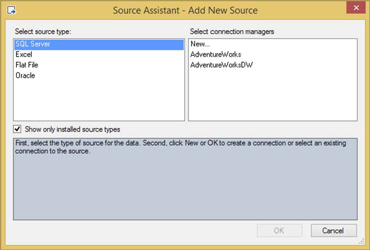
FIGURE 4-1
OLE DB Source
The OLE DB Source is the most common type of source, and it can point to any OLE DB–compliant Data Source such as SQL Server, Oracle, or DB2. To configure the OLE DB Source, double-click the source once you have added it to the design pane in the Data Flow tab. In the Connection Manager page of the OLE DB Source Editor (see Figure 4-2), select the Connection Manager of your OLE DB Source from the OLE DB Connection Manager dropdown box. You can also add a new Connection Manager in the editor by clicking the New button.
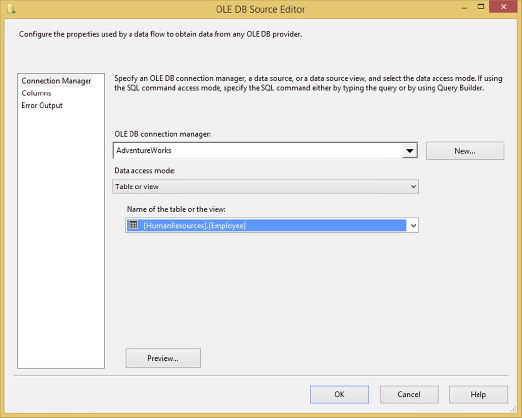
FIGURE 4-2
The “Data access mode” option specifies how you wish to retrieve the data. Your options here are Table/View or SQL Command, or you can pull either from a package variable. Once you select the data access mode, you need the table or view, or you can type a query. For multiple reasons that will be explained momentarily, it is a best practice to retrieve the data from a query. This query can also be a stored procedure. Additionally, you can pass parameters into the query by substituting a question mark (?) for where the parameter should be and then clicking the Parameters button. You’ll learn more about parameterization of your queries in Chapter 5.
As with most sources, you can go to the Columns page to set columns that you wish to output to the Data Flow, as shown in Figure 4-3. Simply check the columns you wish to output, and you can then assign the name you want to send down the Data Flow in the Output column. Select only the columns that you want to use, because the smaller the data set, the better the performance you will get.
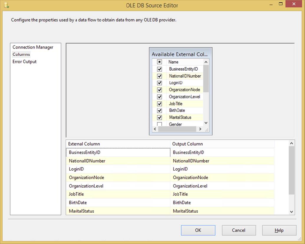
FIGURE 4-3
From a performance perspective, this is a case where it’s better to have typed the query in the Connection Manager page rather than to have selected a table. Selecting a table to pull data from essentially selects all columns and all rows from the target table, transporting all that data across the network. Then, going to the Columns page and unchecking the unnecessary columns applies a client-side filter on the data, which is not nearly as efficient as selecting only the necessary columns in the SQL query. This is also gentler on the amount of buffers you fill as well.
Optionally, you can go to the Error Output page (shown in Figure 4-4) and specify how you wish to handle rows that have errors. For example, you may wish to output any rows that have a data type conversion issue to a different path in the Data Flow. On each column, you can specify that if an error occurs, you wish the row to be ignored, be redirected, or fail. If you choose to ignore failures, the column for that row will be set to NULL. If you redirect the row, the row will be sent down the red path in the Data Flow coming out of the OLE DB Source.
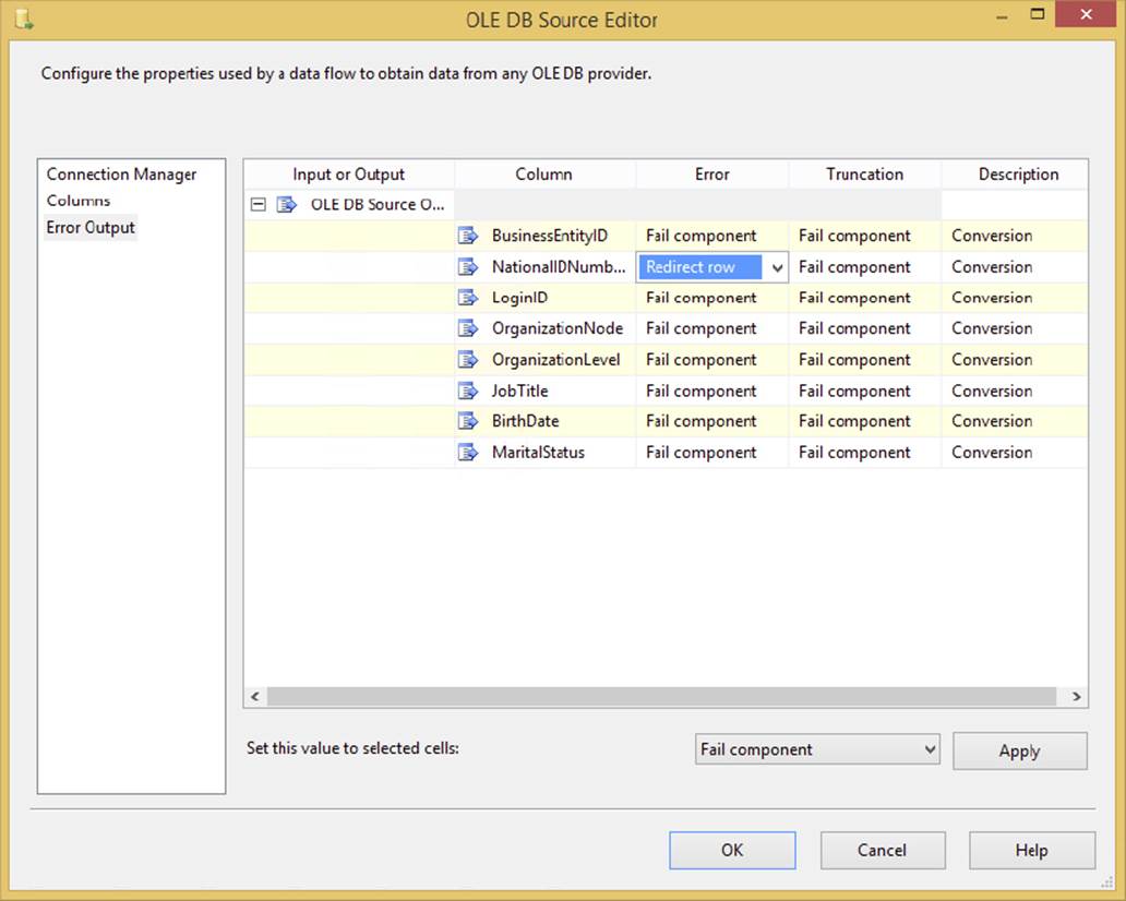
FIGURE 4-4
The Truncation column specifies what to do if data truncation occurs. A truncation error would happen, for example, if you try to place 200 characters of data into a column in the Data Flow that supports only 100. You have the same options available to you for Truncation as you do for the Error option. By default, if an error occurs with data types or truncation, an error will occur, causing the entire Data Flow to fail.
Excel Source
The Excel Source is a source component that points to an Excel spreadsheet, just like it sounds. Once you point to an Excel Connection Manager, you can select the sheet from the “Name of the Excel sheet” dropdown box, or you can run a query by changing the Data Access Mode. This source treats Excel just like a database, where an Excel sheet is the table and the workbook is the database. If you do not see a list of sheets in the dropdown box, you may have a 64-bit machine that needs the ACE driver installed or you need to run the package in 32-bit mode. How to do this is documented in the next section in this chapter.
SSIS supports Excel data types, but it may not support them the way you wish by default. For example, the default format in Excel is General. If you right-click a column and select Format Cells, you’ll find that most of the columns in your Excel spreadsheet have probably been set to General. SSIS translates this general format as a Unicode string data type. In SQL Server, Unicode translates into nvarchar, which is probably not what you want. If you have a Unicode data type in SSIS and you try to insert it into a varchar column, it will potentially fail. The solution is to place a Data Conversion Transformation between the source and the destination in order to change the Excel data types. You can read more about Data Conversion Transformations later in this chapter.
Excel 64-Bit Scenarios
If you are connecting to an Excel 2007 spreadsheet or later, ensure that you select the proper Excel version when creating the Excel Connection Manager. You will not be able to connect to an Excel 2007, Excel 2010, or Excel 2013 spreadsheet otherwise. Additionally, the default Excel driver is a 32-bit driver only, and your packages have to run in 32-bit mode when using Excel connectivity. In the designer, you would receive the following error message if you do not have the correct driver installed:
The 'Microsoft.ACE.OLEDB.12.0' provider is not registered on the local machine.
To fix this, simply locate this driver on the Microsoft site and you’ll be able to run packages with an Excel source in 64-bit.
Flat File Source
The Flat File Source provides a data source for connections such as text files or data that’s delimited. Flat File Sources are typically comma- or tab-delimited files, or they could be fixed-width or ragged-right. A fixed-width file is typically received from the mainframe or government entities and has fixed start and stop points for each column. This method enables a fast load, but it takes longer at design time for the developer to map each column. You specify a Flat File Source the same way you specify an OLE DB Source. Once you add it to your Data Flow pane, you point it to a Connection Manager connection that is a flat file or a multi-flat file. Next, from the Columns tab, you specify which columns you want to be presented to the Data Flow. All the specifications for the flat file, such as delimiter type, were previously set in the Flat File Connection Manager.
In this example, you’ll create a Connection Manager that points to a file called FactSales.csv, which you can download from this book’s website at www.wrox.com/go/prossis2014. The file has a date column, a few string columns, integer columns, and a currency column. Because of the variety of data types it includes, this example presents an interesting case study for learning how to configure a Flat File Connection Manager.
First, right-click in the Connection Manager area of the Package Designer and select New Flat File Connection Manager. This will open the Flat File Connection Manager Editor, as shown in Figure 4-5. Name the Connection Manager Fact Sales and point it to wherever you placed the FactSales.csv file. Check the “Column names in the first data row” option, which specifies that the first row of the file contains a header row with the column names.
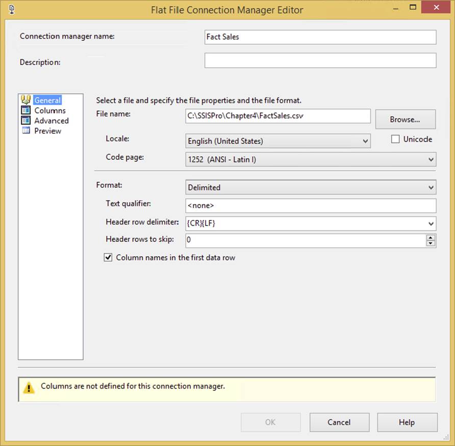
FIGURE 4-5
Another important option is the “Text qualifier” option. Although there isn’t one for this file, sometimes your comma-delimited files may require that you have a text qualifier. A text qualifier places a character around each column of data to show that any comma delimiter inside that symbol should be ignored. For example, if you had the most common text qualifier of double-quotes around your data, a row may look like the following, whereby there are only three columns even though the commas may indicate five:
"Knight,Brian", 123, "Jacksonville, FL"
In the Columns page of the Connection Manager, you can specify what will delimit each column in the flat file if you chose a delimited file. The row delimiter specifies what will indicate a new row. The default option is a carriage return followed by a line feed. The Connection Manager’s file is automatically scanned to determine the column delimiter and, as shown in Figure 4-6, use a tab delimiter for the example file.
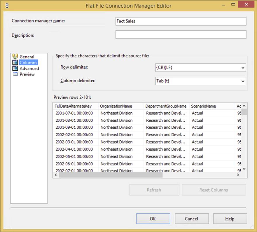
FIGURE 4-6
NOTE Often, once you make a major change to your header delimiter or your text qualifier, you’ll have to click the Reset Columns button. Doing so requeries the file in order to obtain the new column names. If you click this option, though, all your metadata in the Advanced page will be recreated as well, and you may lose a sizable amount of work.
The Advanced page of the Connection Manager is the most important feature in the Connection Manager. In this tab, you specify the data type for each column in the flat file and the name of the column, as shown in Figure 4-7. This column name and data type will be later sent to the Data Flow. If you need to change the data types or names, you can always come back to the Connection Manager, but be aware that you need to open the Flat File Source again to refresh the metadata.
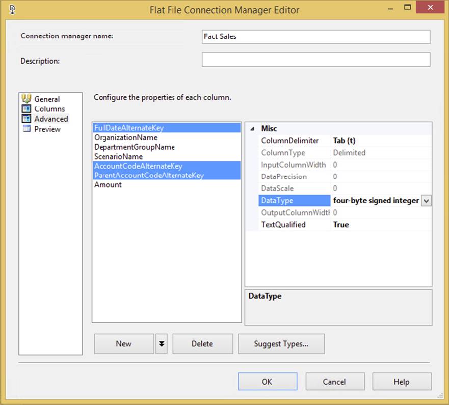
FIGURE 4-7
NOTE Making a change to the Connection Manager’s data types or columns requires that you refresh any Data Flow Task using that Connection Manager. To do so, open the Flat File Source Editor, which will prompt you to refresh the metadata of the Data Flow. Answer yes, and the metadata will be corrected throughout the Data Flow.
If you don’t want to specify the data type for each individual column, you can click the Suggest Types button on this page to have SSIS scan the first 100 records (by default) in the file to guess the appropriate data types. Generally speaking, it does a bad job at guessing, but it’s a great place to start if you have a lot of columns.
If you prefer to do this manually, select each column and then specify its data type. You can also hold down the Ctrl key or Shift key and select multiple columns at once and change the data types or column length for multiple columns at the same time.
A Flat File Connection Manager initially treats each column as a 50-character string by default. Leaving this default behavior harms performance when you have a true integer column that you’re trying to insert into SQL Server, or if your column contains more data than 50 characters of data. The settings you make in the Advanced page of the Connection Manager are the most important work you can do to ensure that all the data types for the columns are properly defined. You should also keep the data types as small as possible. For example, if you have a zip code column that’s only 9 digits in length, define it as a 9-character string. This will save an additional 41 bytes in memory multiplied by however many rows you have.
A frustrating point with SSIS sometimes is how it deals with SQL Server data types. For example, a varchar maps in SSIS to a string column. It was designed this way to translate well into the .NET development world and to provide an agnostic product. The following table contains some of the common SQL Server data types and what they are mapped into in a Flat File Connection Manager.
|
SQL SERVER DATA TYPE |
CONNECTION MANAGER DATA TYPE |
|
Bigint |
Eight-byte signed integer [DT_I8] |
|
Binary |
Byte stream [DT_BYTES] |
|
Bit |
Boolean [DT_BOOL] |
|
Tinyint |
Single-byte unsigned integer [DT_UI1] |
|
Datetime |
Database timestamp [DT_DBTIMESTAMP] |
|
Decimal |
Numeric [DT_NUMERIC] |
|
Real |
Float [DT_R4] |
|
Int |
Four-byte signed integer [DT_I4] |
|
Image |
Image [DT_IMAGE] |
|
Nvarchar or nchar |
Unicode string [DT_WSTR] |
|
Ntext |
Unicode text stream [DT_NTEXT] |
|
Numeric |
Numeric [DT_NUMERIC] |
|
Smallint |
Two-byte signed integer [DT_I2] |
|
Text |
Text stream [DT_TEXT] |
|
Timestamp |
Byte stream [DT_BYTES] |
|
Uniqueidentifier |
Unique identifier [DT_GUID] |
|
Varbinary |
Byte stream [DT_BYTES] |
|
Varchar or char |
String [DT_STR] |
|
Xml |
Unicode string [DT_WSTR] |
FastParse Option
By default, SSIS issues a contract between the Flat File Source and a Data Flow. It states that the source component must validate any numeric or date column. For example, if you have a flat file in which a given column is set to a four-byte integer, every row must first go through a short validation routine to ensure that it is truly an integer and that no character data has passed through. On date columns, a quick check is done to ensure that every date is indeed a valid in-range date.
This validation is fast but it does require approximately 20 to 30 percent more time to validate that contract. To set the FastParse property, go into the Data Flow Task for which you’re using a Flat File Source. Right-click the Flat File Source and select Show Advanced Editor. From there, select the Input and Output Properties tab, and choose any number or date column under Flat File Output ⇒ Output Columns tree. In the right pane, change the FastParse property to True, as shown in Figure 4-8.
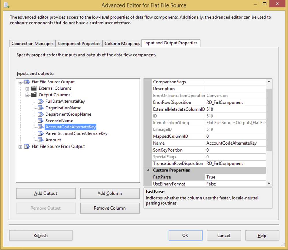
FIGURE 4-8
MultiFlatFile Connection Manager
If you know that you want to process a series of flat files in a Data Flow, or you want to refer to many files in the Control Flow, you can optionally use the MultiFlatFile or “Multiple Flat File Connection Manager.” The Multiple Flat File Connection Manager refers to a list of files for copying or moving, or it may hold a series of SQL scripts to execute, similar to the File Connection Manager. The Multiple Flat File Connection Manager gives you the same view as a Flat File Connection Manager, but it enables you to point to multiple files. In either case, you can point to a list of files by placing a vertical bar (|) between each filename:
C:\Projects\011305c.dat|C:\Projects\053105c.dat
In the Data Flow, the Multiple Flat File Connection Manager reacts by combining the total number of records from all the files that you have pointed to, appearing like a single merged file. Using this option will initiate the Data Flow process only once for the files whereas the Foreach Loop container will initiate the process once per file being processed. In either case, the metadata from the file must match in order to use them in the Data Flow. Most developers lean toward using Foreach Loop Containers because it’s easier to make them dynamic. With these Multiple File or Multiple Flat File Connection Managers, you have to parse your file list and add the vertical bar between them. If you use Foreach Loop Containers, that is taken care of for you.
Raw File Source
The Raw File Source is a specialized type of file that is optimized for reading data quickly from SSIS. A Raw File Source is created by a Raw File Destination (discussed later in this chapter). You can’t add columns to the Raw File Source, but you can remove unused columns from the source in much the same way you do in the other sources. Because the Raw File Source requires little translation, it can load data much faster than the Flat File Source, but the price of this speed is little flexibility. Typically, you see raw files used to capture data at checkpoints to be used later in case of a package failure.
These sources are typically used for cross-package or cross-Data Flow communication. For example, if you have a Data Flow that takes four hours to run, you might wish to stage the data to a raw file halfway through the processing in case a problem occurs. Then, the second Data Flow Task would continue the remaining two hours of processing.
XML Source
The XML source is a powerful SSIS source that can use a local or remote (via HTTP or UNC) XML file as the source. This source component is a bit different from the OLE DB Source in its configuration. First, you point to the XML file locally on your machine or at a UNC path. You can also point to a remote HTTP address for an XML file. This is useful for interaction with a vendor. This source is also very useful when used in conjunction with the Web Service Task or the XML Task. Once you point the data item to an XML file, you must generate an XSD (XML Schema Definition) file by clicking the Generate XSD button or point to an existing XSD file. The schema definition can also be an in-line XML file, so you don’t necessarily need an XSD file. Each of these cases may vary based on the XML that you’re trying to connect. The rest of the source resembles other sources; for example, you can filter the columns you don’t want to see down the chain.
ADO.NET Source
The ADO.NET Source enables you to make a .NET provider a source and make it available for consumption inside the package. The source uses an ADO.NET Connection Manager to connect to the provider. The Data Flow is based on OLE DB, so for best performance, using the OLE DB Source is preferred. However, some providers might require that you use the ADO.NET source. Its interface is identical in appearance to the OLE DB Source, but it does require an ADO.NET Connection Manager.
DESTINATIONS
Inside the Data Flow, destinations accept the data from the Data Sources and from the transformations. The architecture can send the data to nearly any OLE DB–compliant Data Source, a flat file, or Analysis Services, to name just a few. Like sources, destinations are managed through Connection Managers. The configuration difference between sources and destinations is that in destinations, you have a Mappings page (shown in Figure 4-9), where you specify how the inputted data from the Data Flow maps to the destination. As shown in the Mappings page in this figure, the columns are automatically mapped based on column names, but they don’t necessarily have to be exactly lined up. You can also choose to ignore given columns, such as when you’re inserting into a table that has an identity column, and you don’t want to inherit the value from the source table.
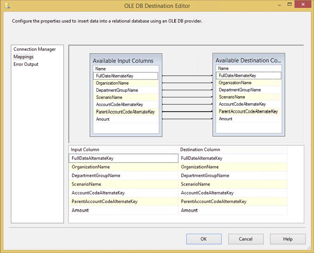
FIGURE 4-9
In SQL Server 2014, you can start by configuring the destination first, but it would lack the metadata you need. So, you will really want to connect to a Data Flow path. To do this, select the source or a transformation and drag the blue arrow to the destination. If you want to output bad data or data that has had an error to a destination, you would drag the red arrow to that destination. If you try to configure the destination before attaching it to the transformation or source, you will see the error in Figure 4-10. In SQL Server 2014, you can still proceed and edit the component, but it won’t be as meaningful without the live metadata.
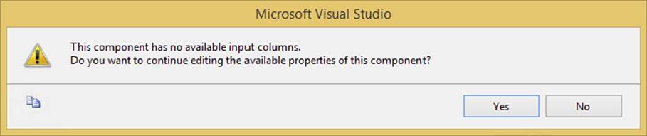
FIGURE 4-10
Excel Destination
The Excel Destination is identical to the Excel Source except that it accepts data rather than sends data. To use it, first select the Excel Connection Manager from the Connection Manager page, and then specify the worksheet into which you wish to load data.
WARNING The big caveat with the Excel Destination is that unlike the Flat File Destination, an Excel spreadsheet must already exist with the sheet into which you wish to copy data. If the spreadsheet doesn’t exist, you will receive an error. To work around this issue, you can create a blank spreadsheet to use as your template, and then use the File System Task to copy the file over.
Flat File Destination
The commonly used Flat File Destination sends data to a flat file, and it can be fixed-width or delimited based on the Connection Manager. The destination uses a Flat File Connection Manager. You can also add a custom header to the file by typing it into the Header option in the Connection Manager page. Lastly, you can specify on this page that the destination file should be overwritten each time the Data Flow is run.
OLE DB Destination
Your most commonly used destination will probably be the OLE DB Destination (see Figure 4-11). It can write data from the source or transformation to OLE DB–compliant Data Sources such as Oracle, DB2, Access, and SQL Server. It is configured like any other destination and source, using OLE DB Connection Managers. A dynamic option it has is the Data Access Mode. If you select Table or View - Fast Load, or its variable equivalent, several options will be available, such as Table Lock. This Fast Load option is available only for SQL Server database instances and turns on a bulk load option in SQL Server instead of a row-by-row operation.
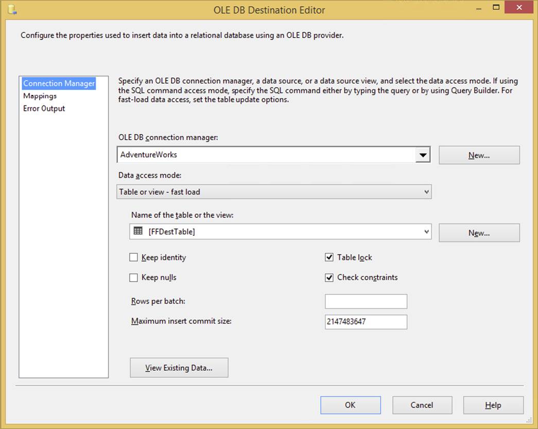
FIGURE 4-11
A few options of note here are Rows Per Batch, which specifies how many rows are in each batch sent to the destination, and Maximum Insert Commit Size, which specifies how large the batch size will be prior to issuing a commit statement. The Table Lock option places a lock on the destination table to speed up the load. As you can imagine, this causes grief for your users if they are trying to read from the table at the same time. Another important option is Keep Identity, which enables you to insert into a column that has the identity property set on it. Generally speaking, you can improve performance by setting Max Insert Commit Size to a number like 10,000, but that number will vary according to column width.
New users commonly ask what the difference is between the fast load and the normal load (table or view option) for the OLE DB Destination. The Fast Load option specifies that SSIS will load data in bulk into the OLE DB Destination’s target table. Because this is a bulk operation, error handling via a redirection or ignoring data errors is not allowed. If you require this level of error handling, you need to turn off bulk loading of the data by selecting Table or View for the Data Access Mode option. Doing so will allow you to redirect your errors down the red line, but it causes a slowdown of the load by a factor of at least four.
Raw File Destination
The Raw File Destination is an especially speedy Data Destination that does not use a Connection Manager to configure. Instead, you point to the file on the server in the editor. This destination is written to typically as an intermediate point for partially transformed data. Once written to, other packages can read the data in by using the Raw File Source. The file is written in native format, so it is very fast.
Recordset Destination
The Recordset Destination populates an ADO recordset that can be used outside the transformation. For example, you can populate the ADO recordset, and then a Script Task could read that recordset by reading a variable later in the Control Flow. This type of destination does not support an error output like some of the other destinations.
Data Mining Model Training
The Data Mining Model Training Destination can train (the process of a data mining algorithm learning the data) an Analysis Services data mining model by passing it data from the Data Flow. You can train multiple mining models from a single destination and Data Flow. To use this destination, you select an Analysis Services Connection Manager and the mining model. Analysis Services mining models are beyond the scope of this book; for more information, please see Professional SQL Server Analysis Services 2012 with MDX and DAX by Sivakumar Harinath and his coauthors (Wrox, 2012).
NOTE The data you pass into the Data Mining Model Training Destination must be presorted. To do this, you use the Sort Transformation, discussed later in this chapter.
DataReader Destination
The DataReader Destination provides a way to extend SSIS Data Flows to external packages or programs that can use the DataReader interface, such as a .NET application. When you configure this destination, ensure that its name is something that’s easy to recognize later in your program, because you will be calling that name later. After you have configured the name and basic properties, check the columns you’d like outputted to the destination in the Input Columns tab.
Dimension and Partition Processing
The Dimension Processing Destination loads and processes an Analysis Services dimension. You have the option to perform full, incremental, or update processing. To configure the destination, select the Analysis Services Connection Manager that contains the dimension you would like to process on the Connection Manager page of the Dimension Processing Destination Editor. You will then see a list of dimensions and fact tables in the box. Select the dimension you want to load and process, and from the Mappings page, map the data from the Data Flow to the selected dimension. Lastly, you can configure how you would like to handle errors, such as unknown keys, in the Advanced page. Generally, the default options are fine for this page unless you have special error-handling needs. The Partition Processing Destination has identical options, but it processes an Analysis Services partition instead of a dimension.
COMMON TRANSFORMATIONS
Transformations or transforms are key components to the Data Flow that transform the data to a desired format as you move from step to step. For example, you may want a sampling of your data to be sorted and aggregated. Three transformations can accomplish this task for you: one to take a random sampling of the data, one to sort, and another to aggregate. The nicest thing about transformations in SSIS is that they occur in-memory and no longer require elaborate scripting as in SQL Server 2000 DTS. As you add a transformation, the data is altered and passed down the path in the Data Flow. Also, because this is done in-memory, you no longer have to create staging tables to perform most functions. When dealing with very large data sets, though, you may still choose to create staging tables.
You set up the transformation by dragging it onto the Data Flow tab design area. Then, click the source or transformation you’d like to connect it to, and drag the green arrow to the target transformation or destination. If you drag the red arrow, then rows that fail to transform will be directed to that target. After you have the transformation connected, you can double-click it to configure it.
Synchronous versus Asynchronous Transformations
Transformations are divided into two main categories: synchronous and asynchronous. In SSIS, you want to ideally use all synchronous components. Synchronous transformations are components such as the Derived Column and Data Conversion Transformations, where rows flow into memory buffers in the transformation, and the same buffers come out. No rows are held, and typically these transformations perform very quickly, with minimal impact to your Data Flow.
Asynchronous transformations can cause a block in your Data Flow and slow down your runtime. There are two types of asynchronous transformations: partially blocking and fully blocking.
· Partially blocking transformations, such as the Union All, create new memory buffers for the output of the transformation.
· Fully blocking transformations, such as the Sort and Aggregate Transformations, do the same thing but cause a full block of the data. In order to sort the data, SSIS must first see every single row of the data. If you have a 100MB file, then you may require 200MB of RAM in order to process the Data Flow because of a fully blocking transformation. These fully blocking transformations represent the single largest slowdown in SSIS and should be considered carefully in terms of any architecture decisions you must make.
NOTE Chapter 16 covers these concepts in much more depth.
Aggregate
The fully blocking asynchronous Aggregate Transformation allows you to aggregate data from the Data Flow to apply certain T-SQL functions that are done in a GROUP BY statement, such as Average, Minimum, Maximum, and Count. For example, in Figure 4-12, you can see that the data is grouped together on the ProductKey column, and then the SalesAmount column is summed. Lastly, for every ProductKey, the maximum OrderDateKey is aggregated. This produces four new columns that can be consumed down the path, or future actions can be performed on them and the other columns dropped at that time.
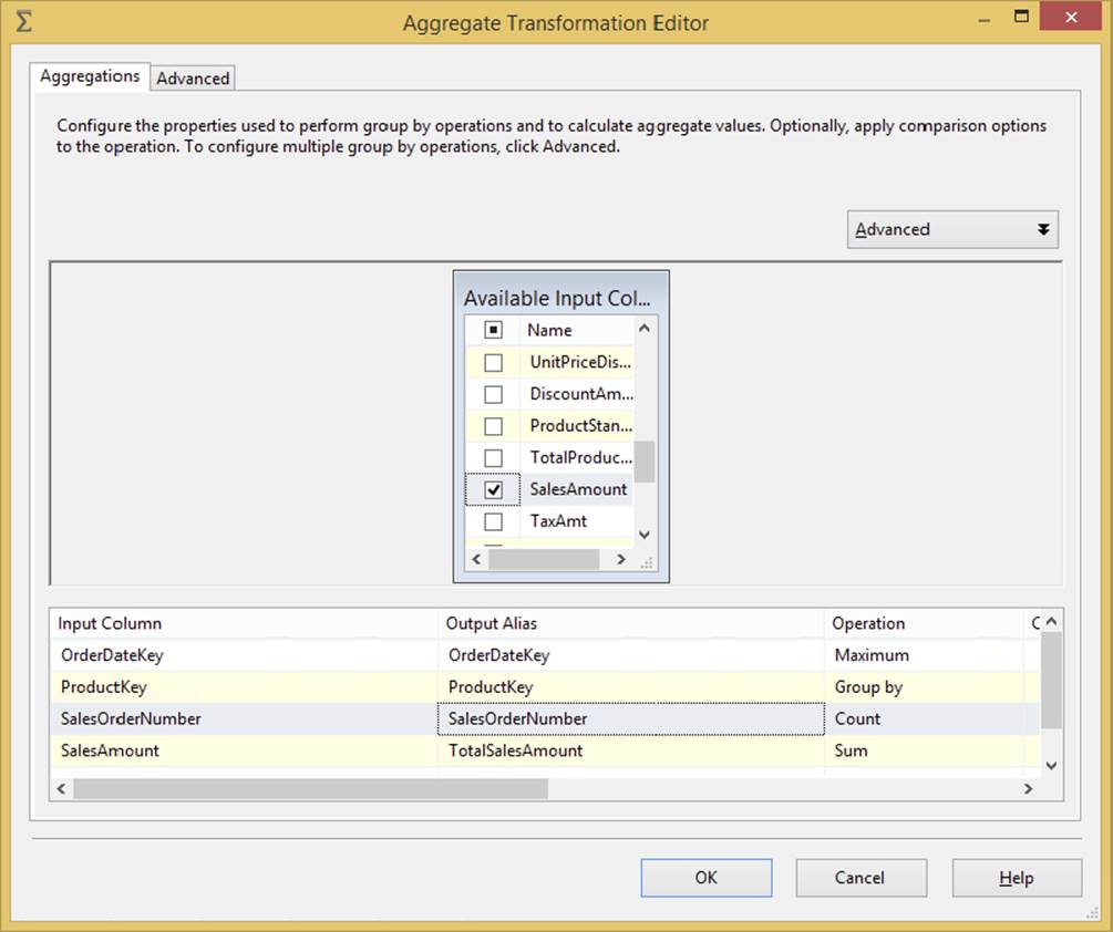
FIGURE 4-12
The Aggregate Transformation is configured in the Aggregate Transformation Editor (see Figure 4-12). To do so, first check the column on which you wish to perform the action. After checking the column, the input column will be filled below in the grid. Optionally, type an alias in the Output Alias column that you wish to give the column when it is outputted to the next transformation or destination. For example, if the column currently holds the total money per customer, you might change the name of the column that’s outputted from SalesAmount to TotalCustomerSaleAmt. This will make it easier for you to recognize what the column represents along the data path. The most important option is Operation. For this option, you can select the following:
· Group By: Breaks the data set into groups by the column you specify
· Average: Averages the selected column’s numeric data
· Count: Counts the records in a group
· Count Distinct: Counts the distinct non-NULL values in a group
· Minimum: Returns the minimum numeric value in the group
· Maximum: Returns the maximum numeric value in the group
· Sum: Returns sum of the selected column’s numeric data in the group
You can click the Advanced tab to see options that enable you to configure multiple outputs from the transformation. After you click Advanced, you can type a new Aggregation Name to create a new output. You will then be able to check the columns you’d like to aggregate again as if it were a new transformation. This can be used to roll up the same input data different ways.
In the Advanced tab, the “Key scale” option sets an approximate number of keys. The default is Unspecified, which optimizes the transformation’s cache to the appropriate level. For example, setting this to Low will optimize the transform to write 500,000 keys. Setting it to Medium will optimize it for 5,000,000 keys, and High will optimize the transform for 25,000,000 keys. You can also set the exact number of keys by using the “Number of keys” option.
The “Count distinct scale” option will optionally set the amount of distinct values that can be written by the transformation. The default value is Unspecified, but if you set it to Low, the transformation will be optimized to write 500,000 distinct values. Setting the option to Medium will set it to 5,000,000 values, and High will optimize the transformation to 25,000,000. The Auto Extend Factor specifies to what factor your memory can be extended by the transformation. The default option is 25 percent, but you can specify another setting to keep your RAM from getting away from you.
Conditional Split
The Conditional Split Transformation is a fantastic way to add complex logic to your Data Flow. This transformation enables you to send the data from a single data path to various outputs or paths based on conditions that use the SSIS expression language. For example, you could configure the transformation to send all products with sales that have a quantity greater than 500 to one path, and products that have more than 50 sales down another path. Lastly, if neither condition is met, the sales would go down a third path, called “Small Sale,” which essentially acts as an ELSE statement in T-SQL. This exact situation is shown in Figure 4-13. You can drag and drop the column or expression code snippets from the tree in the top-right panel. After you complete the condition, you need to name it something logical, rather than the default name of Case 1. You’ll use this case name later in the Data Flow. You also can configure the “Default output name,” which will output any data that does not fit any case. Each case in the transform and the default output name will show as a green line in the Data Flow and will be annotated with the name you typed in.
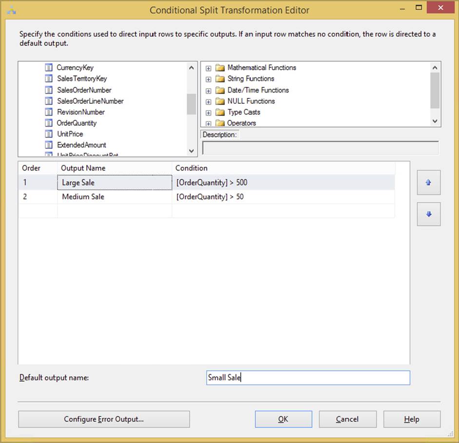
FIGURE 4-13
You can also conditionally read string data by using SSIS expressions, such as the following example, which reads the first letter of the City column:
SUBSTRING(City,1,1) == "F"
You can learn much more about the expression language in Chapter 5. Once you connect the transformation to the next transformation in the path or destination, you’ll see a pop-up dialog that lets you select which case you wish to flow down this path, as shown inFigure 4-14. In this figure, you can see three cases. The “Large Sale” condition can go down one path, “Medium Sales” down another, and the default “Small Sales” down the last path. After you complete the configuration of the first case, you can create a path for each case in the conditional split.
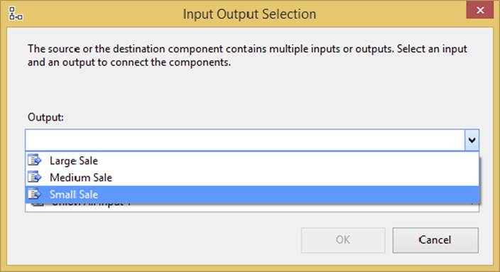
FIGURE 4-14
A much more detailed example of the Conditional Split Transformation is given in Chapter 8.
Data Conversion
The Data Conversion Transformation performs a similar function to the CONVERT or CAST functions in T-SQL. This transformation is configured in the Data Conversion Transformation Editor (see Figure 4-15), where you check each column that you wish to convert and then specify to what you wish to convert it under the Data Type column. The Output Alias is the column name you want to assign to the column after it is transformed. If you don’t assign it a new name, it will later be displayed as Data Conversion: ColumnName in the Data Flow. This same logic can also be accomplished in a Derived Column Transform, but this component provides a simpler UI.
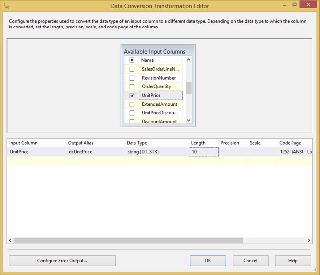
FIGURE 4-15
Derived Column
The Derived Column Transformation creates a new column that is calculated (derived) from the output of another column or set of columns. It is one of the most important transformations in your Data Flow arsenal. You may wish to use this transformation, for example, to multiply the quantity of orders by the cost of the order to derive the total cost of the order, as shown in Figure 4-16. You can also use it to find out the current date or to fill in the blanks in the data by using the ISNULL function. This is one of the top five transformations that you will find yourself using to alleviate the need for T-SQL scripting in the package.
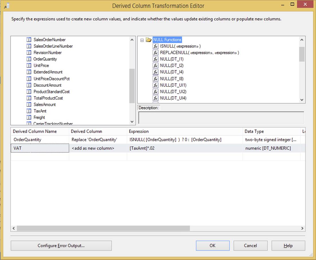
FIGURE 4-16
To configure this transformation, drag the column or variable into the Expression column, as shown in Figure 4-16. Then add any functions to it. You can find a list of functions in the top-right corner of the Derived Column Transformation Editor. You must then specify, in the Derived Column dropdown box, whether you want the output to replace an existing column in the Data Flow or create a new column. As shown in Figure 4-16, the first derived column expression is doing an in-place update of the OrderQuantity column. The expression states that if the OrderQuantity column is null, then convert it to 0; otherwise, keep the existing data in the OrderQuantity column. If you create a new column, specify the name in the Derived Column Name column, as shown in the VAT column.
You’ll find all the available functions for the expression language in the top-right pane of the editor. There are no hidden or secret expressions in this C# variant expression language. We use the expression language much more throughout this and future chapters so don’t worry too much about the details of the language yet.
Some common expressions can be found in the following table:
|
EXAMPLE EXPRESSION |
DESCRIPTION |
|
SUBSTRING(ZipCode, 1,5) |
Captures the first 5 numbers of a zip code |
|
ISNULL(Name) ? “NA” : Name |
If the Name column is NULL, replace with the value of NA. Otherwise, keep the Name column as is. |
|
UPPER(FirstName) |
Uppercases the FirstName column |
|
(DT_WSTR, 3)CompanyID + Name |
Converts the CompanyID column to a string and appends it to the Name column |
Lookup
The Lookup Transformation performs what equates to an INNER JOIN on the Data Flow and a second data set. The second data set can be an OLE DB table or a cached file, which is loaded in the Cache Transformation. After you perform the lookup, you can retrieve additional columns from the second column. If no match is found, an error occurs by default. You can later choose, using the Configure Error Output button, to ignore the failure (setting any additional columns retrieved from the reference table to NULL) or redirect the rows down the second nonmatched green path.
NOTE This is a very detailed transformation; it is covered in much more depth in Chapter 7 and again in Chapter 8.
Cache
The Cache Transformation enables you to load a cache file on disk in the Data Flow. This cache file is later used for fast lookups in a Lookup Transformation. The Cache Transformation can be used to populate a cache file in the Data Flow as a transformation, and then be immediately used, or it can be used as a destination and then used by another package or Data Flow in the same package.
The cache file that’s created enables you to perform lookups against large data sets from a raw file. It also enables you to share the same lookup cache across many Data Flows or packages.
NOTE This transformation is covered in much more detail in Chapter 7.
Row Count
The Row Count Transformation provides the capability to count rows in a stream that is directed to its input source. This transformation must place that count into a variable that could be used in the Control Flow — for insertion into an audit table, for example. This transformation is useful for tasks that require knowing “how many?” It is especially valuable because you don’t physically have to commit stream data to a physical table to retrieve the count, and it can act as a destination, terminating your data stream. If you need to know how many rows are split during the Conditional Split Transformation, direct the output of each side of the split to a separate Row Count Transformation. Each Row Count Transformation is designed for an input stream and will output a row count into a Long (integer) or compatible data type. You can then use this variable to log information into storage, to build e-mail messages, or to conditionally run steps in your packages.
For this transformation, all you really need to provide in terms of configuration is the name of the variable to store the count of the input stream. You will now simulate a row count situation in a package. You could use this type of logic to implement conditional execution of any task, but for simplicity you’ll conditionally execute a Script Task that does nothing.
1. Create an SSIS package named Row Count Example. Add a Data Flow Task to the Control Flow design surface.
2. In the Control Flow tab, add a variable named iRowCount. Ensure that the variable is package scoped and of type Int32. If you don’t know how to add a variable, select Variable from the SSIS menu and click the Add Variable button.
3. Create a Connection Manager that connects to the AdventureWorks database. Add an OLE DB Data Source to the Data Flow design surface. Configure the source to point to your AdventureWorks database’s Connection Manager and the table [ErrorLog].
4. Add a Row Count Transformation Task to the Data Flow tab. Open the Advanced Editor. Select the variable named User::iRowCount as the Variable property. Your editor should resemble Figure 4-17.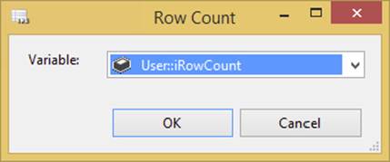
FIGURE 4-17
5. Return to the Control Flow tab and add a Script Task. This task won’t really perform any action. It will be used to show the conditional capability to perform steps based on the value returned by the Row Count Transformation.
6. Connect the Data Flow Task to the Script Task.
7. Right-click the arrow connecting the Data Flow and Script Tasks. Select the Edit menu. In the Precedence Constraint Editor, change the Evaluation Operation to Expression. Set the Expression to @iRowCount>0.
When you run the package, you’ll see that the Script Task is not executed. If you are curious, insert a row into the [ErrorLog] table and rerun the package or change the source table that has data. You’ll see that the Script Task will show a green checkmark, indicating that it was executed. An example of what your package may look like is shown in Figure 4-18. In this screenshot, no rows were transformed, so the Script Task never executed.
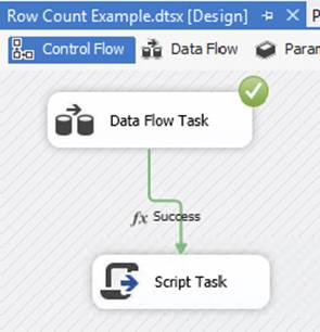
FIGURE 4-18
Script Component
The Script Component enables you to write custom .NET scripts as transformations, sources, or destinations. Once you drag the component over, it will ask you if you want it to be a source, transformation, or destination. Some of the things you can do with this transformation include the following:
· Create a custom transformation that would use a .NET assembly to validate credit card numbers or mailing addresses.
· Validate data and skip records that don’t seem reasonable. For example, you can use it in a human resource recruitment system to pull out candidates that don’t match the salary requirement at a job code level.
· Read from a proprietary system for which no standard provider exists.
· Write a custom component to integrate with a third-party vendor.
Scripts used as sources can support multiple outputs, and you have the option of precompiling the scripts for runtime efficiency.
NOTE You can learn much more about the Script Component in Chapter 9.
Slowly Changing Dimension
The Slowly Changing Dimension (SCD) Transformation provides a great head start in helping to solve a common, classic changing-dimension problem that occurs in the outer edge of your data model — the dimension or lookup tables. The changing-dimension issue in online transaction and analytical processing database designs is too big to cover in this chapter, but a brief overview should help you understand the value of service the SCD Transformation provides.
A dimension table contains a set of discrete values with a description and often other measurable attributes such as price, weight, or sales territory. The classic problem is what to do in your dimension data when an attribute in a row changes — particularly when you are loading data automatically through an ETL process. This transformation can shave days off of your development time in relation to creating the load manually through T-SQL, but it can add time because of how it queries your destination and how it updates with the OLE DB Command Transform (row by row).
NOTE Loading data warehouses is covered in Chapter 12.
Sort
The Sort Transformation is a fully blocking asynchronous transformation that enables you to sort data based on any column in the path. This is probably one of the top ten transformations you will use on a regular basis because some of the other transformations require sorted data, and you’re reading data from a system that does not allow you to perform an ORDER BY clause or is not pre-sorted. To configure it, open the Sort Transformation Editor after it is connected to the path and check the column that you wish to sort by. Then, uncheck any column you don’t want passed through to the path from the Pass Through column. By default, every column will be passed through the pipeline. You can see this in Figure 4-19, where the user is sorting by the Name column and passing all other columns in the path as output.
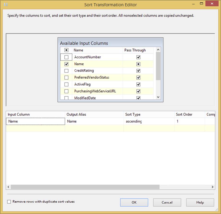
FIGURE 4-19
In the bottom grid, you can specify the alias that you wish to output and whether you want to sort in ascending or descending order. The Sort Order column shows which column will be sorted on first, second, third, and so on. You can optionally check the Remove Rows with Duplicate Sort Values option to “Remove rows that have duplicate sort values.” This is a great way to do rudimentary de-duplication of your data. If a second value comes in that matches your same sort key, it is ignored and the row is dropped.
NOTE Because this is an asynchronous transformation, it will slow down your Data Flow immensely. Use it only when you have to, and use it sparingly.
As mentioned previously, avoid using the Sort Transformation when possible, because of speed. However, some transformations, like the Merge Join and Merge, require the data to be sorted. If you place an ORDER BY statement in the OLE DB Source, SSIS is not aware of the ORDER BY statement because it could just have easily been in a stored procedure.
If you have an ORDER BY clause in your T-SQL statement in the OLE DB Source or the ADO.NET Source, you can notify SSIS that the data is already sorted, obviating the need for the Sort Transformation in the Advanced Editor. After ordering the data in your SQL statement, right-click the source and select Advanced Editor. From the Input and Output Properties tab, select OLE DB Source Output. In the Properties pane, change the IsSorted property to True.
Then, under Output Columns, select the column you are ordering on in your SQL statement, and change the SortKeyPosition to 1 if you’re sorting only by a single column ascending, as shown in Figure 4-20. If you have multiple columns, you could change this SortKeyPosition value to the column position in the ORDER BY statement starting at 1. A value of -1 will sort the data in descending order.
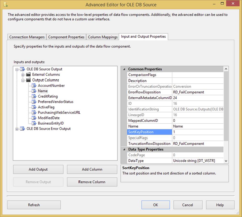
FIGURE 4-20
Union All
The Union All Transformation works much the same way as the Merge Transformation, but it does not require sorted data. It takes the outputs from multiple sources or transformations and combines them into a single result set. For example, in Figure 4-21, the user combines the data from three sources into a single output using the Union All Transformation. Notice that the City column is called something different in each source and that all are now merged in this transformation into a single column. Think of the Union All as essentially stacking the data on top of each other, much like the T-SQL UNION operator does.
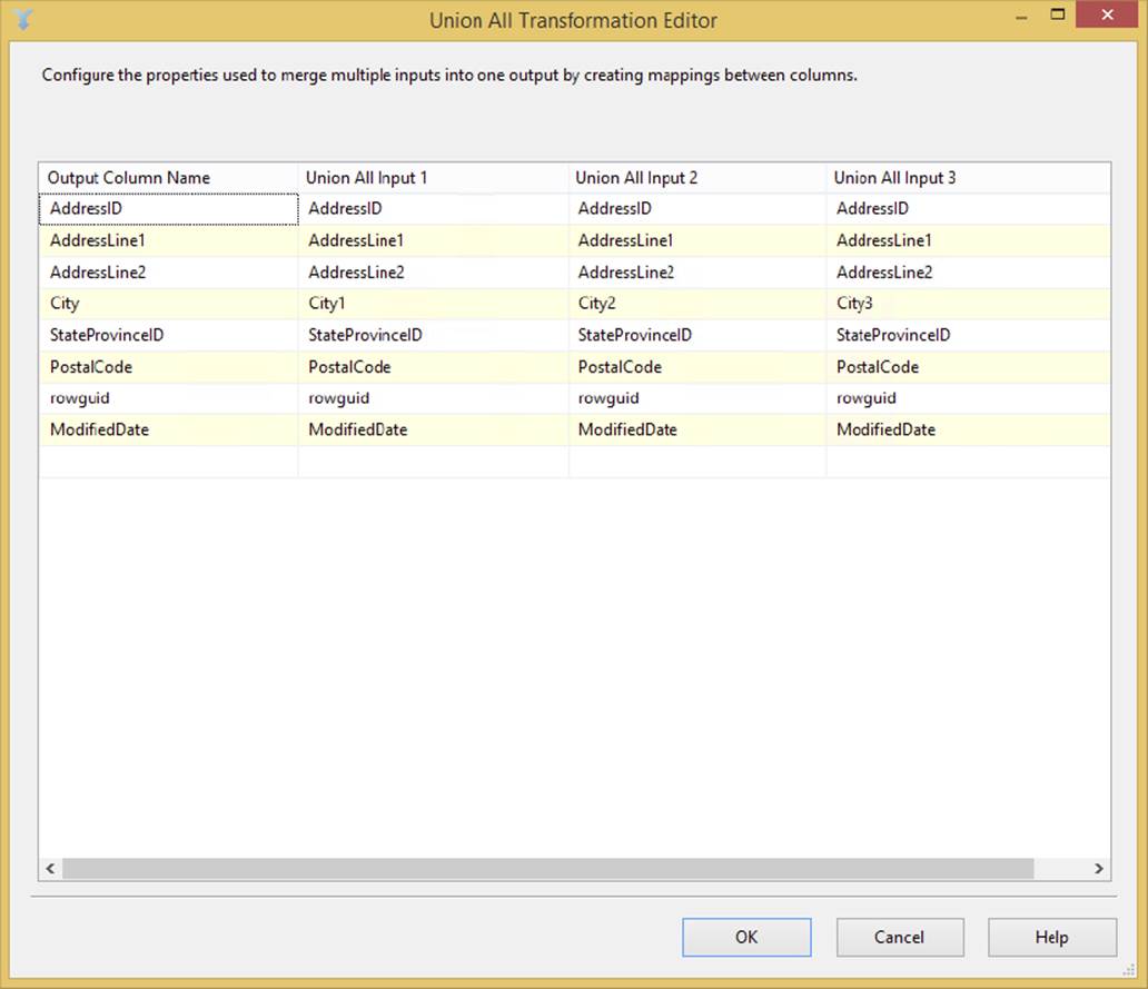
FIGURE 4-21
To configure the transformation, connect the first source or transformation to the Union All Transformation, and then continue to connect the other sources or transformations to it until you are done. You can optionally open the Union All Transformation Editor to ensure that the columns map correctly, but SSIS takes care of that for you automatically. The transformation fixes minor metadata issues. For example, if you have one input that is a 20-character string and another that is 50 characters, the output of this from the Union All Transformation will be the longer 50-character column. You need to open the Union All Transformation Editor only if the column names from one of the transformations that feed the Union All Transformation have different column names.
OTHER TRANSFORMATIONS
There are many more transformations you can use to complete your more complex Data Flow. Some of these transformations like the Audit and Case Transformations can be used in lieu of a Derived Column Transformation because they have a simpler UI. Others serve a purpose that’s specialized.
Audit
The Audit Transformation allows you to add auditing data to your Data Flow. Because of acts such as HIPPA and Sarbanes-Oxley (SOX) governing audits, you often must be able to track who inserted data into a table and when. This transformation helps you with that function. The task is easy to configure. For example, to track what task inserted data into the table, you can add those columns to the Data Flow path with this transformation. The functionality in the Audit Transformation can be achieved with a Derived Column Transformation, but the Audit Transformation provides an easier interface.
All other columns are passed through to the path as an output, and any auditing item you add will also be added to the path. Simply select the type of data you want to audit in the Audit Type column (shown in Figure 4-22), and then name the column that will be outputted to the flow. Following are some of the available options:
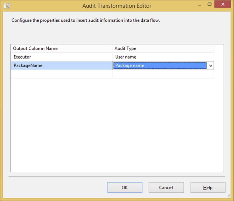
FIGURE 4-22
· Execution instance GUID: GUID that identifies the execution instance of the package
· Package ID: Unique ID for the package
· Package name: Name of the package
· Version ID: Version GUID of the package
· Execution start time: Time the package began
· Machine name: Machine on which the package ran
· User name: User who started the package
· Task name: Data Flow Task name that holds the Audit Task
· Task ID: Unique identifier for the Data Flow Task that holds the Audit Task
Character Map
The Character Map Transformation (shown in Figure 4-23) performs common character translations in the flow. This simple transformation can be configured in a single tab. To do so, check the columns you wish to transform. Then, select whether you want this modified column to be added as a new column or whether you want to update the original column. You can give the column a new name under the Output Alias column. Lastly, select the operation you wish to perform on the inputted column. The available operation types are as follows:
· Byte Reversal: Reverses the order of the bytes. For example, for the data 0x1234 0x9876, the result is 0x4321 0x6789. This uses the same behavior as LCMapString with the LCMAP_BYTEREV option.
· Full Width: Converts the half-width character type to full width
· Half Width: Converts the full-width character type to half width
· Hiragana: Converts the Katakana style of Japanese characters to Hiragana
· Katakana: Converts the Hiragana style of Japanese characters to Katakana
· Linguistic Casing: Applies the regional linguistic rules for casing
· Lowercase: Changes all letters in the input to lowercase
· Traditional Chinese: Converts the simplified Chinese characters to traditional Chinese
· Simplified Chinese: Converts the traditional Chinese characters to simplified Chinese
· Uppercase: Changes all letters in the input to uppercase
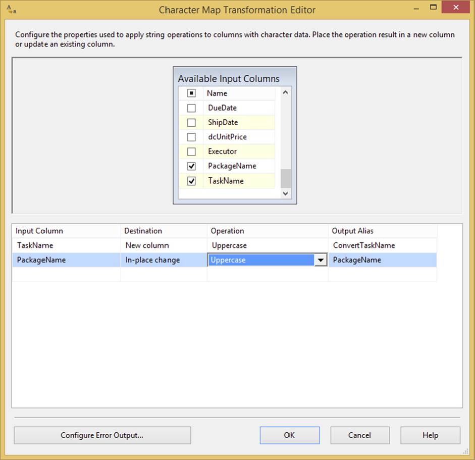
FIGURE 4-23
In Figure 4-23, you can see that two columns are being transformed — both to uppercase. For the TaskName input, a new column is added, and the original is kept. The PackageName column is replaced in-line.
Copy Column
The Copy Column Transformation is a very simple transformation that copies the output of a column to a clone of itself. This is useful if you wish to create a copy of a column before you perform some elaborate transformations. You could then keep the original value as your control subject and the copy as the modified column. To configure this transformation, go to the Copy Column Transformation Editor and check the column you want to clone. Then assign a name to the new column.
NOTE The Derived Column Transformation will allow you to transform the data from a column to a new column, but the UI in the Copy Column Transformation is simpler for some.
Data Mining Query
The Data Mining Query Transformation typically is used to fill in gaps in your data or predict a new column for your Data Flow. This transformation runs a Data Mining Extensions (DMX) query against an SSAS data-mining model, and adds the output to the Data Flow. It also can optionally add columns, such as the probability of a certain condition being true. A few great scenarios for this transformation would be the following:
· You could take columns, such as number of children, household income, and marital income, to predict a new column that states whether the person owns a house or not.
· You could predict what customers would want to buy based on their shopping cart items.
· You could fill the gaps in your data where customers didn’t enter all the fields in a questionnaire.
The possibilities are endless with this transformation.
DQS Cleansing
The Data Quality Services (DQS) Cleansing Transformation performs advanced data cleansing on data flowing through it. With this transformation, you can have your business analyst (BA) create a series of business rules that declare what good data looks like in the Data Quality Client (included in SQL Server). The BA will use a tool called the Data Quality Client to create domains that define data in your company, such as what a Company Name column should always look like. The DQS Cleansing Transformation can then use that business rule.
This transformation will score the data for you and tell you what the proper cleansed value should be. Chapter 10 covers this transformation in much more detail.
Export Column
The Export Column Transformation is a transformation that exports data to a file from the Data Flow. Unlike the other transformations, the Export Column Transformation doesn’t need a destination to create the file. To configure it, go to the Export Column Transformation Editor, shown in Figure 4-24. Select the column that contains the file from the Extract Column dropdown box. Select the column that contains the path and filename to send the files to in the File Path Column dropdown box.
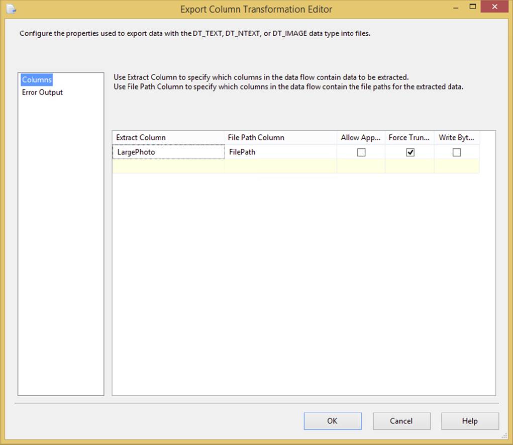
FIGURE 4-24
The other options specify where the file will be overwritten or dropped. The Allow Append checkbox specifies whether the output should be appended to the existing file, if one exists. If you check Force Truncate, the existing file will be overwritten if it exists. The Write BOM option specifies whether a byte-order mark is written to the file if it is a DT_NTEXT or DT_WSTR data type.
If you do not check the Append or Truncate options and the file exists, the package will fail if the error isn’t handled. The following error is a subset of the complete error you would receive:
Error: 0xC02090A6 at Data Flow Task, Export Column [61]: Opening the file
"wheel_small.tif" for writing failed. The file exists and cannot be
overwritten. If the AllowAppend property is FALSE and the ForceTruncate
property is set to FALSE, the existence of the file will cause this failure.
The Export Column Transformation Task is used to extract blob-type data from fields in a database and create files in their original formats to be stored in a file system or viewed by a format viewer, such as Microsoft Word or Microsoft Paint. The trick to understanding the Export Column Transformation is that it requires an input stream field that contains digitized document data, and another field that can be used for a fully qualified path. The Export Column Transformation will convert the digitized data into a physical file on the file system for each row in the input stream using the fully qualified path.
In the following example, you’ll use existing data in the AdventureWorksDW database to output some stored documents from the database back to file storage. The database has a table named DimProduct that contains a file path and a field containing an embedded Microsoft Word document. Pull these documents out of the database and save them into a directory on the file system.
1. Create a directory with an easy name like c:\ProSSIS\Chapter4\Export that you can use when exporting these pictures.
2. Create a new SSIS project and package named Export Column Example.dtsx. Add a Data Flow Task to the Control Flow design surface.
3. On the Data Flow design surface, add an OLE DB Data Source configured to the AdventureWorksDW database table DimProduct.
4. Add a Derived Column Transformation Task to the Data Flow design surface. Connect the output of the OLE DB data to the task.
5. Create a Derived Column Name named FilePath. Use the Derived Column setting of <add as new column>. To derive a new filename, just use the primary key for the filename and add your path to it. To do this, set the expression to the following:
"c:\ProSSIS\Chapter4\Export\" + (DT_WSTR,50)ProductKey + ".gif"
NOTE The \\ is required in the expressions editor instead of \ because of its use as an escape sequence.
6. Add an Export Column Transformation Task to the Data Flow design surface. Connect the output of the Derived Column Task to the Export Column Transformation Task, which will consume the input stream and separate all the fields into two usable categories: fields that can possibly be in digitized data formats, and fields that can possibly be used as filenames.
7. Set the Extract Column equal to the [LargePhoto] field, since this contains the embedded GIF image. Set the File Path Column equal to the field name [FilePath]. This field is the one that you derived in the Derived Column Task.
8. Check the Force Truncate option to rewrite the files if they exist. (This will enable you to run the package again without an error if the files already exist.)
9. Run the package and check the contents of the directory. You should see a list of image files in primary key sequence.
Fuzzy Lookup
If you have done some work in the world of extract, transfer, and load (ETL) processes, then you’ve run into the proverbial crossroads of handling bad data. The test data is staged, but all attempts to retrieve a foreign key from a dimension table result in no matches for a number of rows. This is the crossroads of bad data. At this point, you have a finite set of options. You could create a set of hand-coded complex lookup functions using SQL Sound-Ex, full-text searching, or distance-based word calculation formulas. This strategy is time-consuming to create and test, complicated to implement, and dependent on a given language, and it isn’t always consistent or reusable (not to mention that everyone after you will be scared to alter the code for fear of breaking it). You could just give up and divert the row for manual processing by subject matter experts (that’s a way to make some new friends). You could just add the new data to the lookup tables and retrieve the new keys. If you just add the data, the foreign key retrieval issue is solved, but you could be adding an entry into the dimension table that skews data-mining results downstream. This is what we like to call a lazy-add. This is a descriptive, not a technical, term. A lazy-add would import a misspelled job title like “prasedent” into the dimension table when there is already an entry of “president.” It was added, but it was lazy.
The Fuzzy Lookup and Fuzzy Grouping Transformations add one more road to take at the crossroads of bad data. These transformations allow the addition of a step to the process that is easy to use, consistent, scalable, and reusable, and they will reduce your unmatched rows significantly — maybe even altogether. If you’ve already allowed bad data in your dimension tables, or you are just starting a new ETL process, you’ll want to put the Fuzzy Grouping Transformation to work on your data to find data redundancy. This transformation can examine the contents of a suspect field in a staged or committed table and provide possible groupings of similar words based on provided tolerances. This matching information can then be used to clean up that table. Fuzzy Grouping is discussed later in this chapter.
If you are correcting data during an ETL process, use the Fuzzy Lookup Transformation — my suggestion is to do so only after attempting to perform a regular lookup on the field. This best practice is recommended because Fuzzy Lookups don’t come cheap. They build specialized indexes of the input stream and the reference data for comparison purposes. You can store them for efficiency, but these indexes can use up some disk space or take up some memory if you choose to rebuild them on each run. Storing matches made by the Fuzzy Lookups over time in a translation or pre-dimension table is a great design. Regular Lookup Transformations can first be run against this lookup table and then divert only those items in the Data Flow that can’t be matched to a Fuzzy Lookup. This technique uses Lookup Transformations and translation tables to find matches using INNER JOINs. Fuzzy Lookups whittle the remaining unknowns down if similar matches can be found with a high level of confidence. Finally, if your last resort is to have the item diverted to a subject matter expert, you can save that decision into the translation table so that the ETL process can match it next time in the first iteration.
Using the Fuzzy Lookup Transformation requires an input stream of at least one field that is a string. Internally, the transformation has to be configured to connect to a reference table that will be used for comparison. The output to this transformation will be a set of columns containing the following:
· Input and Pass-Through Field Names and Values: This column contains the name and value of the text input provided to the Fuzzy Lookup Transformation or passed through during the lookup.
· Reference Field Name and Value: This column contains the name and value(s) of the matched results from the reference table.
· Similarity: This column contains a number between 0 and 1 representing similarity to the matched row and column. Similarity is a threshold that you set when configuring the Fuzzy Lookup Task. The closer this number is to 1, the closer the two text fields must match.
· Confidence: This column contains a number between 0 and 1 representing confidence of the match relative to the set of matched results. Confidence is different from similarity, because it is not calculated by examining just one word against another but rather by comparing the chosen word match against all the other possible matches. For example, the value of Knight Brian may have a low similarity threshold but a high confidence that it matches to Brian Knight. Confidence gets better the more accurately your reference data represents your subject domain, and it can change based on the sample of the data coming into the ETL process.
The Fuzzy Lookup Transformation Editor has three configuration tabs.
· Reference Table: This tab (shown in Figure 4-25) sets up the OLE DB Connection to the source of the reference data. The Fuzzy Lookup takes this reference data and builds a token-based index (which is actually a table) out of it before it can begin to compare items. This tab contains the options to save that index or use an existing index from a previous process. There is also an option to maintain the index, which will detect changes from run to run and keep the index current. Note that if you are processing large amounts of potential data, this index table can grow large.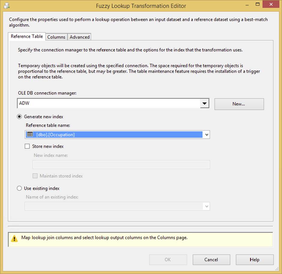
FIGURE 4-25
There are a few additional settings in this tab that are of interest. The default option to set is the “Generate new index” option. By setting this, a table will be created on the reference table’s Connection Manager each time the transformation is run, and that table will be populated with loads of data as mentioned earlier in this section. The creation and loading of the table can be an expensive process. This table is removed after the transformation is complete.
Alternatively, you can select the “Store new index” option, which will instantiate the table and not drop it. You can then reuse that table from other Data Flows or other Data Flows from other packages and over multiple days. As you can imagine, by doing this your index table becomes stale soon after its creation. There are stored procedures you can run to refresh it in SQL, or you can click the “Maintain stored index” checkbox to create a trigger on the underlying reference table to automatically maintain the index table. This is available only with SQL Server reference tables, and it may slow down your insert, update, and delete statements to that table.
· Columns: This tab allows mapping of the one text field in the input stream to the field in the reference table for comparison. Drag and drop a field from the Available Input Column onto the matching field in the Available Lookup Column. You can also click the two fields to be compared and right-click to create a relationship. Another neat feature is the capability to add the foreign key of the lookup table to the output stream. To do this, just click that field in the Available Input Columns.
· Advanced: This tab contains the settings that control the fuzzy logic algorithms. You can set the maximum number of matches to output per incoming row. The default is set to 1, which means pull the best record out of the reference table if it meets the similaritythreshold. Incrementing this setting higher than this may generate more results that you’ll have to sift through, but it may be required if there are too many closely matching strings in your domain data. A slider controls the Similarity threshold. It is recommended that you start this setting at .71 when experimenting and move up or down as you review the results. This setting is normally determined based on a businessperson’s review of the data, not the developer’s review. If a row cannot be found that’s similar enough, the columns that you checked in the Columns tab will be set to NULL. The token delimiters can also be set if, for example, you don’t want the comparison process to break incoming strings up by a period (.) or spaces. The default for this setting is all common delimiters. Figure 4-26 shows an example of an Advanced tab.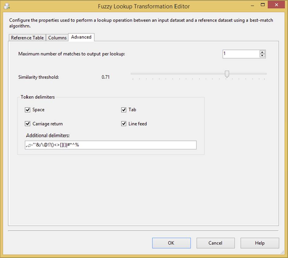
FIGURE 4-26
It’s important to not use Fuzzy Lookup as your primary Lookup Transformation for lookups because of the performance overhead; the Fuzzy Lookup transformation is significantly slower than the Lookup transformation. Always try an exact match using a Lookup Transformation and then redirect nonmatches to the Fuzzy Lookup if you need that level of lookup. Additionally, the Fuzzy Lookup Transformation does require the BI or Enterprise Edition of SQL Server.
Although this transformation neatly packages some highly complex logic in an easy-to-use component, the results won’t be perfect. You’ll need to spend some time experimenting with the configurable settings and monitoring the results. To that end, the following short example puts the Fuzzy Lookup Transformation to work by setting up a small table of occupation titles that will represent your dimension table. You will then import a set of person records that requires a lookup on the occupation to your dimension table. Not all will match, of course. The Fuzzy Lookup Transformation will be employed to find matches, and you will experiment with the settings to learn about its capabilities.
1. Use the following data (code file FuzzyExample.txt) for this next example. This file can also be downloaded from www.wrox.com/go/prossis2014 and saved to c:\ProSSIS\Chapter4\FuzzyExample.txt. The data represents employee information that you are going to import. Notice that some of the occupation titles are cut off in the text file because of the positioning within the layout. Also notice that this file has an uneven right margin. Both of these issues are typical ETL situations that are especially painful.
2. EMPID TITLE LNAME
3. 00001 EXECUTIVE VICE PRESIDEN WASHINGTON
4. 00002 EXEC VICE PRES PIZUR
5. 00003 EXECUTIVE VP BROWN
6. 00005 EXEC VP MILLER
7. 00006 EXECUTIVE VICE PRASIDENS WAMI
8. 00007 FIELDS OPERATION MGR SKY
9. 00008 FLDS OPS MGR JEAN
10. 00009 FIELDS OPS MGR GANDI
11. 00010 FIELDS OPERATIONS MANAG HINSON
12. 00011 BUSINESS OFFICE MANAGER BROWN
13. 00012 BUS OFFICE MANAGER GREEN
14. 00013 BUS OFF MANAGER GATES
15. 00014 BUS OFF MGR HALE
16. 00015 BUS OFFICE MNGR SMITH
17. 00016 BUS OFFICE MGR AI
18. 00017 X-RAY TECHNOLOGIST CHIN
19. 00018 XRAY TECHNOLOGIST ABULA
20. 00019 XRAY TECH HOGAN
00020 X-RAY TECH ROBERSON
21.Run the following SQL code (code file FuzzyExampleInsert.sql) in AdventureWorksDW or another database of your choice. This code will create your dimension table and add the accepted entries that will be used for reference purposes. Again, this file can be downloaded from www.wrox.com/go/prossis2014:
22. CREATE TABLE [Occupation](
23. [OccupationID] [smallint] IDENTITY(1,1) NOT NULL,
24. [OccupationLabel] [varchar] (50) NOT NULL
25. CONSTRAINT [PK_Occupation_OccupationID] PRIMARY KEY CLUSTERED
26. (
27. [OccupationID] ASC
28. ) ON [PRIMARY]
29. ) ON [PRIMARY]
30. GO
31. INSERT INTO [Occupation] Select 'EXEC VICE PRES'
32. INSERT INTO [Occupation] Select 'FIELDS OPS MGR'
33. INSERT INTO [Occupation] Select 'BUS OFFICE MGR'
INSERT INTO [Occupation] Select 'X-RAY TECH'
34.Create a new SSIS package and drop a Data Flow Task on the Control Flow design surface and click the Data Flow tab.
35.Add a Flat File Connection to the Connection Manager. Name it Extract, and then set the filename to c:\projects\Chapter4\fuzzyexample.txt. Set the Format property to Delimited, and set the option to pull the column names from the first data row, as shown inFigure 4-27.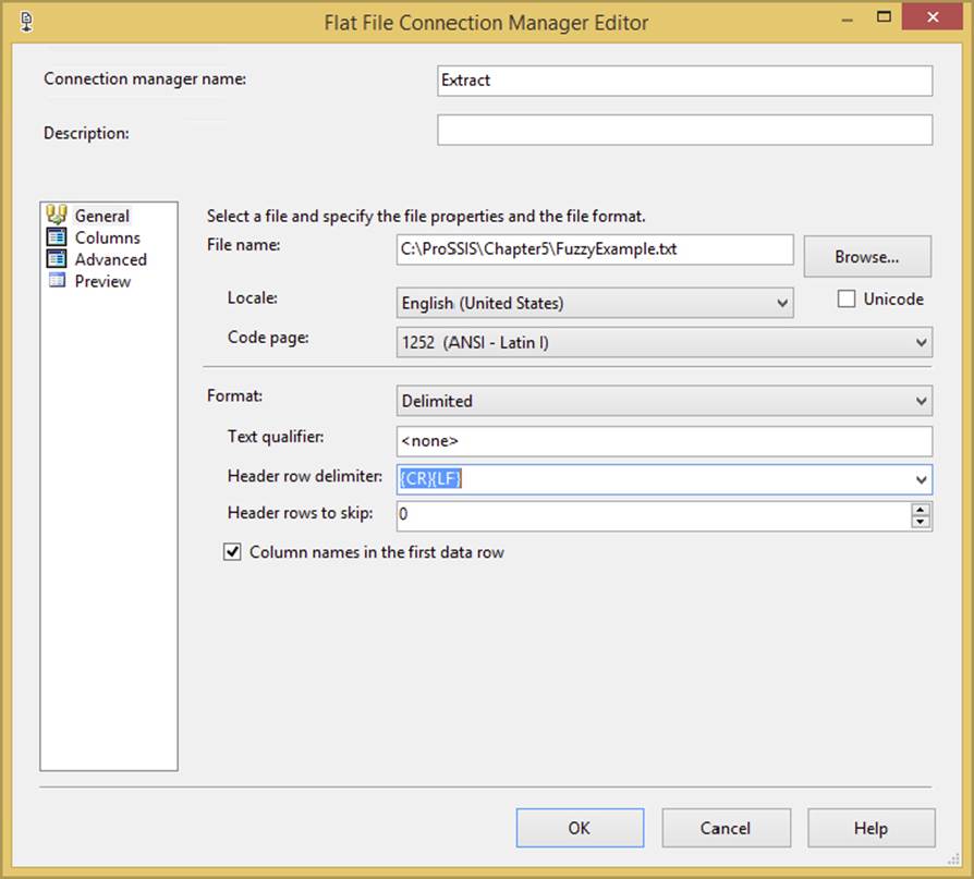
FIGURE 4-27
36.Click the Columns tab to confirm it is properly configured and showing three columns. Click the Advanced tab and ensure the OuputColumnWidth property for the TITLE field is set to 50 characters in length. Save the connection.
37.Add a Flat File Source to the Data Flow surface and configure it to use the Extract connection.
38.Add a Fuzzy Lookup Transformation to the Data Flow design surface. Connect the output of the Flat File Source to the Fuzzy Lookup, and connect the output of the Fuzzy Lookup to the OLE DB Destination.
39.Open the Fuzzy Lookup Transformation Editor. Set the OLE DB Connection Manager in the Reference tab to use the AdventureWorksDW database connection and the Occupation table. Set up the Columns tab by connecting the input to the reference table columns as in Figure 4-28, dragging the Title column to the OccupationLabel column on the right. Set up the Advanced tab with a Similarity threshold of 50 (0.50).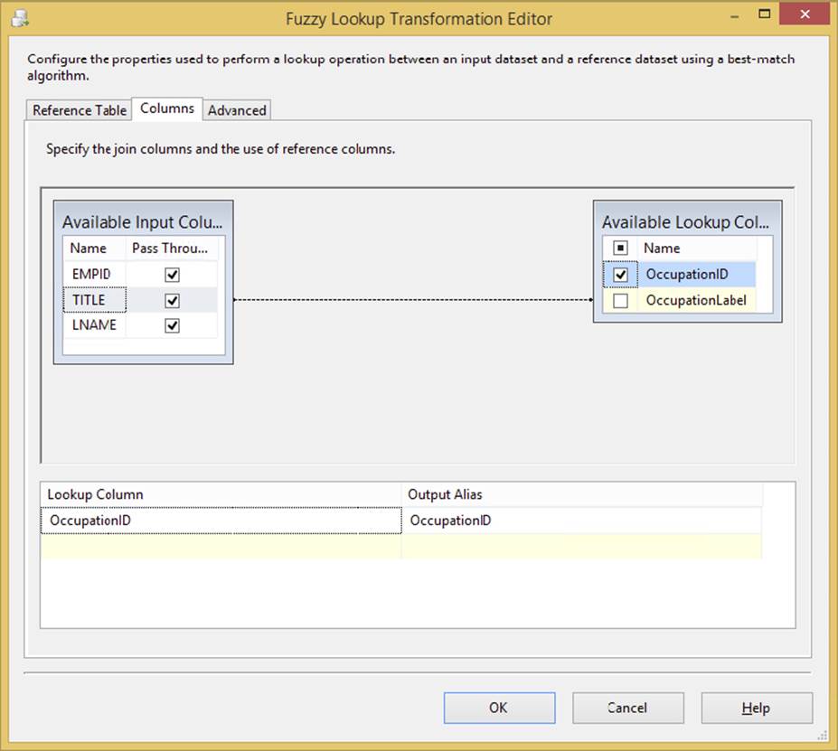
FIGURE 4-28
40.Open the editor for the OLE DB Destination. Set the OLE DB connection to the AdventureWorksDW database. Click New to create a new table to store the results. Change the table name in the DDL statement that is presented to you to create the [FuzzyResults] table. Click the Mappings tab, accept the defaults, and save.
41.Add a Data Viewer of type grid to the Data Flow between the Fuzzy Lookup and the OLE DB Destination.
Run the package. Your results at the Data View should resemble those in Figure 4-29. Notice that the logic has matched most of the items at a 50 percent similarity threshold — and you have the foreign key OccupationID added to your input for free! Had you used a strict INNER JOIN or Lookup Transformation, you would have made only three matches, a dismal hit ratio. These items can be seen in the Fuzzy Lookup output, where the values are 1 for similarity and confidence. A few of the columns are set to NULL now, because the row like Executive VP wasn’t 50 percent similar to the Exec Vice Pres value. You would typically send those NULL records with a conditional split to a table for manual inspection.
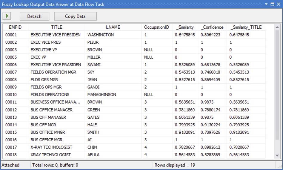
FIGURE 4-29
Fuzzy Grouping
In the previous section, you learned about situations where bad data creeps into your dimension tables. The blame was placed on the “lazy-add” ETL processes that add data to dimension tables to avoid rejecting rows when there are no natural key matches. Processes like these are responsible for state abbreviations like “XX” and entries that look to the human eye like duplicates but are stored as two separate entries. The occupation titles “X-Ray Tech” and “XRay Tech” are good examples of duplicates that humans can recognize but computers have a harder time with.
The Fuzzy Grouping Transformation can look through a list of similar text and group the results using the same logic as the Fuzzy Lookup. You can use these groupings in a transformation table to clean up source and destination data or to crunch fact tables into more meaningful results without altering the underlying data. The Fuzzy Group Transformation also expects an input stream of text, and it requires a connection to an OLE DB Data Source because it creates in that source a set of structures to use during analysis of the input stream.
The Fuzzy Lookup Editor has three configuration tabs:
· Connection Manager: This tab sets the OLE DB connection that the transform will use to write the storage tables that it needs.
· Columns: This tab displays the Available Input Columns and allows the selection of any or all input columns for fuzzy grouping analysis. Figure 4-30 shows a completed Columns tab.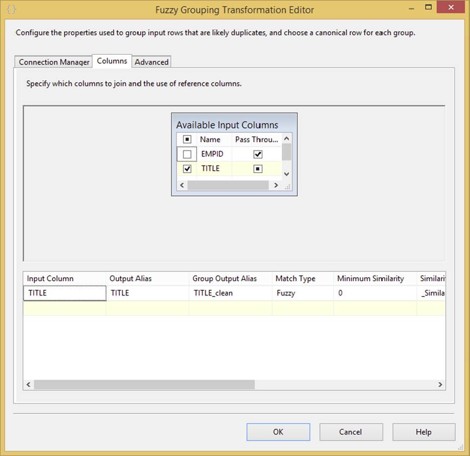
FIGURE 4-30
Each column selected is analyzed and grouped into logical matches, resulting in a new column representing that group match for each data row. Each column can also be selected for Pass-Through — meaning the data is not analyzed, but it is available in the output stream. You can choose the names of any of the output columns: Group Output Alias, Output Alias, Clean Match, and Similarity Alias Score column.
The minimum similarity evaluation is available at the column level if you select more than one column.
The numerals option (which is not visible in Figure 4-30 but can be found by scrolling to the right) enables configuration of the significance of numbers in the input stream when grouping text logically. The options are leading numbers, trailing numbers, leading and trailing numbers, or neither leading nor trailing numbers. This option needs to be considered when comparing addresses or similar types of information.
Comparison flags provide the same options to ignore or pay attention to case, kana type, nonspacing characters, character width, symbols, and punctuation.
· Advanced: This tab contains the settings controlling the fuzzy logic algorithms that assign groupings to text in the input stream. You can set the names of the three additional fields that are added automatically to the output of this transformation. These fields are named _key_in, _key_out, and _score by default. A slider controls the Similarity threshold. The recommended initial setting for this transformation is 0.5, which can be adjusted up or down as you review the results. The token delimiters can also be set if, for example, you don’t want the comparison process to break incoming strings up by a period (.) or spaces. The default for this setting is all common delimiters. Figure 4-31 shows a completed Advanced tab.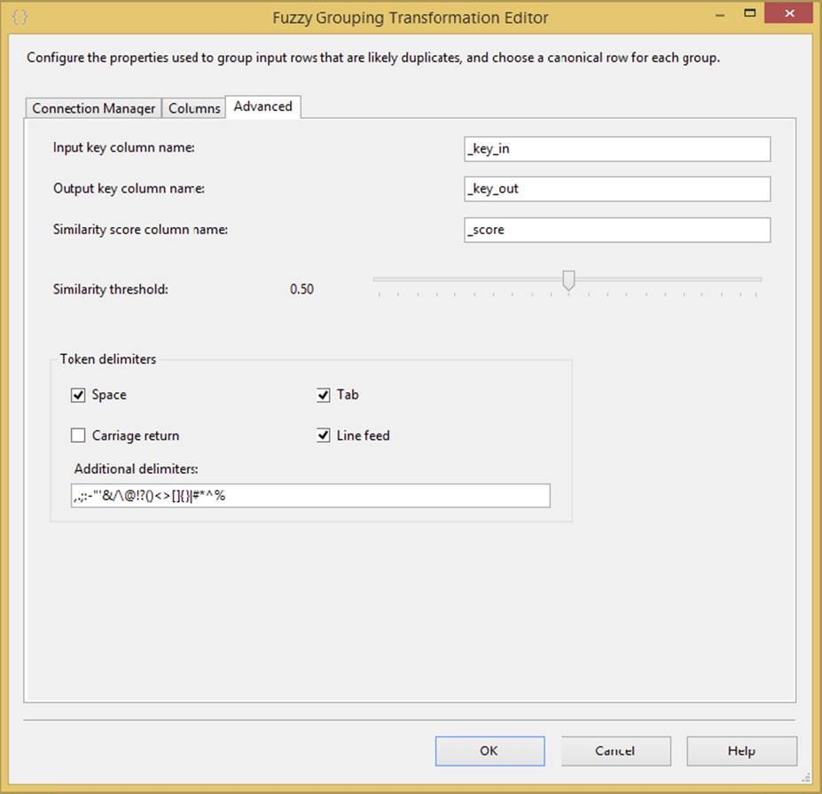
FIGURE 4-31
Suppose you are tasked with creating a brand-new occupations table using the employee occupations text file you imported in the Fuzzy Lookup example. Using only this data, you need to create a new employee occupations table with occupation titles that can serve as natural keys and that best represent this sample. You can use the Fuzzy Grouping Transformation to develop the groupings for the dimension table, like this:
1. Create a new SSIS project named Fuzzy Grouping Example. Drop a Data Flow Task on the Control Flow design surface and click the Data Flow tab.
2. Add a Flat File Connection to the Connection Manager. Name it Extract. Set the filename to c:\ProSSIS\Chapter4\FuzzyExample.txt. (Use the FuzzyExample.txt file from the Fuzzy Lookup example with the same configuration.) Save the connection.
3. Add a Flat File Source to the Data Flow surface and configure it to use the Employee Data connection.
4. Add a Fuzzy Grouping Transformation to the Data Flow design surface. Connect the output of the Flat File Source to the Fuzzy Lookup.
5. Open the Fuzzy Grouping Editor and set the OLE DB Connection Manager to a new AdventureWorksDW connection.
6. In the Columns tab, select the Title column in the Available Input Columns. Accept the other defaults.
7. In the Advanced tab, set the Similarity threshold to 0.50. This will be your starting point for similarity comparisons.
8. Add an OLE DB Destination to the Data Flow design surface. Configure the destination to use the AdventureWorksDW database or another database of your choice. For the Name of Table or View, click the New button. Change the name of the table in the CREATE table statement to [FuzzyGroupingResults]. Click the Mappings tab to complete the task and then save it.
9. Add a Data Viewer in the pipe between the Fuzzy Grouping Transformation and the OLE DB Destination. Set the type to grid so that you can review the data at this point. Run the package. The output shown at various similarity thresholds would look similar toFigure 4-32.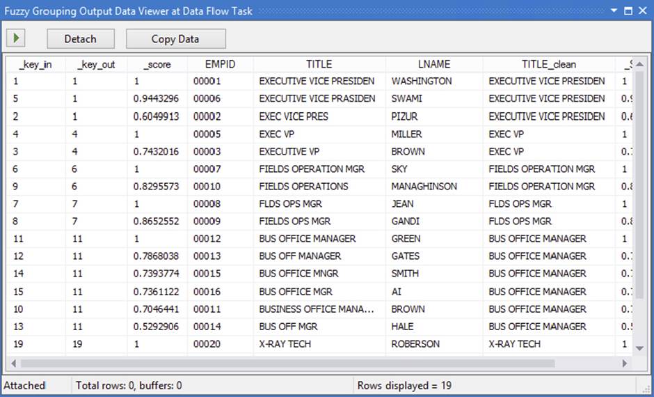
FIGURE 4-32
Now you can look at these results and see more logical groupings and a few issues even at the lowest level of similarity. The title of “X-Ray Tech” is similar to the title “X-Ray Technologist.” The title “Executive Vice Presiden” isn’t a complete title, and really should be grouped with “Exec VP,” but this is pretty good for about five minutes of work.
To build a dimension table from this output, look at the two fields in the Data View named _key_in and _key_out. If these two values match, then the grouped value is the “best” representative candidate for the natural key in a dimension table. Separate the rows in the stream using a Conditional Split Transformation where these two values match, and use an OLE Command Transformation to insert the values in the dimension table. Remember that the more data, the better the grouping.
The output of the Fuzzy Grouping Transformation is also a good basis for a translation table in your ETL processes. By saving both the original value and the Fuzzy Grouping value — with a little subject matter expert editing — you can use a Lookup Transformation and this table to provide much better foreign key lookup results. You’ll be able to improve on this with the Slowly Changing Dimension Transformation later in the chapter.
Import Column
The Import Column Transformation is a partner to the Export Column Transformation. These transformations do the work of translating physical files from system file storage paths into database blob-type fields, and vice versa. The trick to understanding the Import Column Transformation is knowing that its input source requires at least one column that is the fully qualified path to the file you are going to store in the database, and you need a destination column name for the output of the resulting blob and file path string. This transformation also has to be configured using the Advanced Editor. The Advanced Editor is not intuitive, or wizard-like in appearance — hence the name “Advanced” (which, incidentally, you will be once you figure it out). In the editor, you won’t be able to merge two incoming column sources into the full file path; therefore, if your source data for the file paths have the filename separate from the file path, you should use the Merge Transformations to concatenate the columns before connecting that stream to the Import Column Transformation.
In the following example, you’ll import some images into your AdventureWorksDW database. Create a new SSIS package. Transformations live in the Data Flow tab, so add a Data Flow Task to the Control Flow, and then add an Import Column Transformation to the Data Flow surface. To keep this easy, you will complete the following short tasks:
1. Find a small GIF file and copy it three times into c:\ProSSIS\Chapter4\import (or just copy and paste the files from the Export Column example). Change the filenames to 1.gif, 2.gif, and 3.gif.
2. Create a text file with the following content and save it in c:\ProSSIS\Chapter4 as filelist.txt:
3. C:\import\1.Gif
4. C:\import\2.Gif
C:\import\3.Gif
5. Run the following SQL script in AdventureWorks to create a storage location for the image files:
6. CREATE TABLE dbo.tblmyImages
7. (
8. [StoredFilePath] [varchar](50) NOT NULL,
9. [ProdPicture] image
)
10.You are going to use the filelist.txt file as your input stream for the files that you need to load into your database, so add a Flat File Source to your Data Flow surface and configure it to read one column from your filelist.txt flat file. Rename this columnImageFilePath.
Take advantage of the opportunity to open the Advanced Editor on the Flat File Source by clicking the Show Advanced Editor link in the property window or by right-clicking the transformation and selecting Advanced Editor, which looks quite a bit different from the Advanced Editor for a source. Note the difference between this editor and the normal Flat File Editor. The Advanced Editor is stripped down to the core of the Data Flow component — no custom wizards, just an interface sitting directly over the object properties themselves. It is possible to mess these properties up beyond recognition, but even in the worst case you can just drop and recreate the component. Look particularly at the Input and Output Properties of the Advanced Editor.
You didn’t have to use the Advanced Editor to set up the import of the filelist.txt file. However, looking at how the Advanced Editor displays the information will be very helpful when you configure the Import Column Transformation. Notice that you have an External Columns (Input) and Output Columns collection, with one node in each collection named ImageFilePath. This reflects the fact that your connection describes a field called ImageFilePath and that this transformation simply outputs data with the same field name.
Connect the Flat File Source to the Import Column Transformation. Open the Advanced Editor for the Import Column Transformation and click the Input Columns tab. The input stream for this task is the output stream for the flat file. Select the one available column, move to the Input and Output Properties tab, and expand these nodes. This time you don’t have much help. An example of this editor is shown in Figure 4-33.
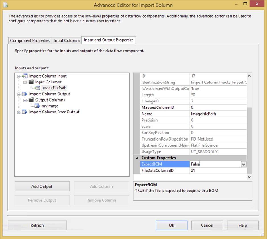
FIGURE 4-33
The Input Columns collection has a column named ImageFilePath, but there are no output columns. On the Flat File Source, you could ignore some of the inputs. In the Import Column Transformation, all inputs have to be re-output. In fact, if you don’t map an output, you’ll get the following error:
Validation error. Data Flow Task: Import Column [1]: The "input column
"ImageFilePath" (164)" references output column ID 0, and that column is not
found on the output.
Add an output column by clicking the Output Columns folder icon and click the Add Column button. Name the column myImage. Notice that the DataType property is [DT_IMAGE] by default. That is because this transformation produces image outputs. You can also pass DT_TEXT, DT_NTEXT, or DT_IMAGE types as outputs from this task. Your last task is to connect the input to the output. Note the output column’s ID property for myImage. This ID needs to be updated in the FileDataColumnID property of the input column ImageFilePath. If you fail to link the output column, you’ll get the following error:
Validation error. Data Flow Task: Import Column [1]: The "output column
"myImage" (207)" is not referenced by any input column. Each output column
must be referenced by exactly one input column.
The Advanced Editor for each of the different transformations has a similar layout but may have other properties available. Another property of interest in this task is Expect BOM, which you would set to True if you expect a byte-order mark at the beginning of the file path (not for this example). A completed editor resembles Figure 4-33.
Complete this example by adding an OLE Destination to the Data Flow design surface. Connect the data from the Import Column to the OLE Destination. Configure the OLE Destination to the AdventureWorksDW database and to the tblmyImages structure that was created for database storage. Click the Mappings setting. Notice that you have two available input columns from the Import Column Task. One is the full path and the other will be the file as type DT_IMAGE. Connect the input and destination columns to complete the transform. Go ahead and run it.
Take a look at the destination table to see the results:
FullFileName Document
---------------------- ------------------------
C:\import\images\1.JPG 0xFFD8FFE120EE45786966000049492A00...
C:\import\images\2.JPG 0xFFD8FFE125FE45786966000049492A00...
C:\import\images\3.JPG 0xFFD8FFE1269B45786966000049492A00...
(3 row(s) affected)
Merge
The Merge Transformation can merge data from two paths into a single output. This transformation is useful when you wish to break out your Data Flow into a path that handles certain errors and then merge it back into the main Data Flow downstream after the errors have been handled. It’s also useful if you wish to merge data from two Data Sources.
This transformation is similar to the Union All Transformation, but the Merge Transformation has some restrictions that may cause you to lean toward using Union All:
· The data must be sorted before the Merge Transformation. You can do this by using the Sort Transformation prior to the merge or by specifying an ORDER BY clause in the source connection.
· The metadata must be the same between both paths. For example, the CustomerID column can’t be a numeric column in one path and a character column in another path.
· If you have more than two paths, you should choose the Union All Transformation.
To configure the transformation, ensure that the data is sorted exactly the same on both paths and drag the path onto the transform. You’ll be asked if the path you want to merge is Merge Input 1 or 2. If this is the first path you’re connecting to the transformation, select Merge Input 1. Next, connect the second path into the transformation. The transformation will automatically configure itself. Essentially, it maps each of the columns to the column from the other path, and you have the option to ignore a certain column’s data.
Merge Join
One of the overriding themes of SSIS is that you shouldn’t have to write any code to create your transformation. This transformation will merge the output of two inputs and perform an INNER or OUTER join on the data. An example of when this would be useful is if you have a front-end web system in one data stream that has a review of a product in it, and you have an inventory product system in another data stream with the product data. You could merge join the two data inputs and output the review and product information into a single path.
NOTE If both inputs are in the same database, then it would be faster to perform a join at the OLE DB Source level, rather than use a transformation through T-SQL. This transformation is useful when you have two different Data Sources you wish to merge, or when you don’t want to write your own join code.
To configure the Merge Join Transformation, connect your two inputs into the Merge Join Transformation, and then select what represents the right and left join as you connect each input. Open the Merge Join Transformation Editor and verify the linkage between the two tables. You can see an example of this in Figure 4-34. You can right-click the arrow to delete a linkage or drag a column from the left input onto the right input to create a new linkage if one is missing. Lastly, check each of the columns you want to be passed as output to the path and select the type of join you wish to make (LEFT, INNER, or FULL).
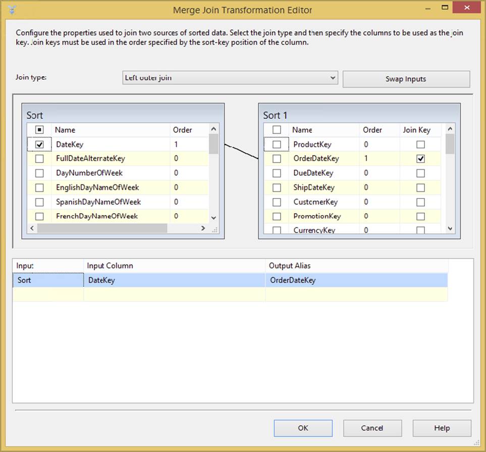
FIGURE 4-34
Multicast
The Multicast Transformation, as the name implies, can send a single data input to multiple output paths easily. You may want to use this transformation to send a path to multiple destinations sliced in different ways. To configure this transformation, simply connect it to your input, and then drag the output path from the Multicast Transformation onto your next destination or transformation. After you connect the Multicast Transformation to your first destination or transformation, you can keep connecting it to other transformations or destinations. There is nothing to configure in the Multicast Transformation Editor other than the names of the outputs.
NOTE The Multicast Transformation is similar to the Conditional Split Transformation in that both transformations send data to multiple outputs. The Multicast will send all the rows down every output path, whereas the Conditional Split will conditionally send each row down exactly one output path.
OLE DB Command
The OLE DB Command Transformation is a component designed to execute a SQL statement for each row in an input stream. This task is analogous to an ADO Command object being created, prepared, and executed for each row of a result set. The input stream provides the data for parameters that can be set into the SQL statement, which is either an in-line statement or a stored procedure call. If you’re like us, just hearing the words “for each row” in the context of SQL makes us think of two other words: performance degradation. This involves firing an update, insert, or delete statement, prepared or unprepared some unknown number of times.
This doesn’t mean there are no good reasons to use this transformation — you’ll actually be doing a few in this chapter. Just understand the impact and think about your use of this transformation. Pay specific attention to the volume of input rows that will be fed into it. Weigh the performance and scalability aspects during your design phases against a solution that would cache the stream into a temporary table and use set-based logic instead.
To use the OLE DB Command Transformation, you basically need to determine how to set up the connection where the SQL statement will be run, provide the SQL statement to be executed, and configure the mapping of any parameters in the input stream to the SQL statement. Take a look at the settings for the OLE DB Command Transformation by opening its editor. The OLE DB Command Transformation is another component that uses the Advanced Editor. There are four tabs in the editor:
· Connection Manager: Allows the selection of an OLE DB Connection. This connection is where the SQL statement will be executed. This doesn’t have to be the same connection that is used to provide the input stream.
· Component Properties: Here you can set the SQL Command statement to be executed in the SQLCommand property, and set the amount of time to allow for a timeout in the CommandTimeout property, in seconds. The property works the same way as the ADO Command object. The value for the CommandTimeout of 0 indicates no timeout. You can also name the task and provide a description in this tab.
· Column Mappings: This tab displays columns available in the input stream and the destination columns, which will be the parameters available in the SQL command. You can map the columns by clicking a column in the input columns and dragging it onto the matching destination parameter. It is a one-to-one mapping, so if you need to use a value for two parameters, you need use a Derived Column Transformation to duplicate the column in the input stream prior to configuring the columns in this transformation.
· Input and Output Properties: Most of the time you’ll be able to map your parameters in the Column Mappings tab. However, if the OLE DB provider doesn’t provide support for deriving parameter information (parameter refreshing), you have to come here to manually set up your output columns using specific parameter names and DBParamInfoFlags.
This transformation should be avoided whenever possible. It’s a better practice to land the data into a staging table using an OLE DB Destination and perform an update with a set-based process in the Control Flow with an Execute SQL Task. The Execute SQL Task’s statement would look something like this if you loaded a table called stg_TransactionHistoryUpdate and were trying to do a bulk update:
BEGIN TRAN
update CDCTransactionHistory
SET TransactionDate = b.TransactionDate,
ActualCost = b.ActualCost
FROM CDCTransactionHistory CDC
INNER JOIN [stg_TransactionHistoryUpdate] b
ON CDC.TransactionID = b.TransactionID
GO
TRUNCATE TABLE [stg_TransactionHistoryUpdate]
COMMIT
If you have 2,000 rows running through the transformation, the stored procedure or command will be executed 2,000 times. It might be more efficient to process these transactions in a SQL batch, but then you would have to stage the data and code the batch transaction. The main problem with this transformation is performance.
Percentage and Row Sampling
The Percentage Sampling and Row Sampling Transformations enable you to take the data from the source and randomly select a subset of data. The transformation produces two outputs that you can select. One output is the data that was randomly selected, and the other is the data that was not selected. You can use this to send a subset of data to a development or test server. The most useful application of this transformation is to train a data-mining model. You can use one output path to train your data-mining model, and the sampling to validate the model.
To configure the transformation, select the percentage or number of rows you wish to be sampled. As you can guess, the Percentage Sampling Transformation enables you to select the percentage of rows, and the Row Sampling Transformation enables you to specify how many rows you wish to be outputted randomly. Next, you can optionally name each of the outputs from the transformation. The last option is to specify the seed that will randomize the data. If you select a seed and run the transformation multiple times, the same data will be outputted to the destination. If you uncheck this option, which is the default, the seed will be automatically incremented by one at runtime, and you will see random data each time.
Pivot Transform
Do you ever get the feeling that pivot tables are the modern-day Rosetta Stone for translating data to your business owners? You store it relationally, but they ask for it in a format that requires you to write a complex case statement to generate. Well, not anymore. Now you can use an SSIS transformation to generate the results. A pivot table is a result of cross-tabulated columns generated by summarizing data from a row format.
Typically, a Pivot Transformation is generated using the following input columns:
· Pivot Key: A pivot column is the element of input data to “pivot.” The word “pivot” is another way of saying “to create a column for each unique instance of.” However, this data must be under control. Think about creating columns in a table. You wouldn’t create 1,000 uniquely named columns in a table, so for best results when choosing a data element to pivot, pick an element that can be run through a GROUP BY statement that will generate 15 or fewer columns. If you are dealing with dates, use something like a DATENAMEfunction to convert to the month or day of the year.
· Set Key: Set key creates one column and places all the unique values for all rows into this column. Just like any GROUP BY statement, some of the data is needed to define the group (row), whereas other data is just along for the ride.
· Pivot Value: These columns are aggregations for data that provide the results in the matrix between the row columns and the pivot columns.
The Pivot Transformation can accept an input stream, use your definitions of the preceding columns, and generate a pivot table output. It helps if you are familiar with your input needs and format your data prior to this transformation. Aggregate the data using GROUP BY statements. Pay special attention to sorting by row columns — this can significantly alter your results.
To set your expectations properly, you have to define each of your literal pivot columns. A common misconception, and source of confusion, is approaching the Pivot Transformation with the idea that you can simply set the pivot column to pivot by the month of the purchase date column, and the transformation should automatically build 12 pivot columns with the month of the year for you. It will not. It is your task to create an output column for each month of the year. If you are using colors as your pivot column, you need to add an output column for every possible color. For example, if columns are set up for blue, green, and yellow, and the color red appears in the input source, then the Pivot Transformation will fail. Therefore, plan ahead and know the possible pivots that can result from your choice of a pivot column or provide for an error output for data that doesn’t match your expected pivot values.
In this example, you’ll use some of the AdventureWorks product and transactional history to generate a quick pivot table to show product quantities sold by month. This is a typical upper-management request, and you can cover all the options with this example. AdventureWorks Management wants a listing of each product with the total quantity of transactions by month for the year 2003.
First identify the pivot column. The month of the year looks like the data that is driving the creation of the pivot columns. The row data columns will be the product name and the product number. The value field will be the total number of transactions for the product in a matrix by month. Now you are ready to set up the Pivot Transformation:
1. Create a new SSIS project named Pivot Example. Add a Data Flow Task to the Control Flow design surface.
2. Add an OLE DB Source to the Data Flow design surface. Configure the connection to the AdventureWorks database. Set the Data Access Mode to SQL Command. Add the following SQL statement (code file PivotExample.sql) to the SQL Command text box:
3. SELECT p.[Name] as ProductName, p.ProductNumber,
4. datename(mm, t.TransactionDate) as TransMonth,
5. sum(t.quantity) as TotQuantity
6. FROM production.product p
7. INNER JOIN production.transactionhistory t
8. ON t.productid = p.productid
9. WHERE t.transactiondate between '01/01/03' and '12/31/03'
10. GROUP BY p.[name], p.productnumber, datename(mm,t.transactiondate)
ORDER BY productname, datename(mm, t.transactiondate)
11.Add the Pivot Transformation and connect the output of the OLE DB Source to the input of the transformation. Open the transformation to edit it.
12.Select TransMonth for the Pivot Key. This is the column that represents your columns. Change the Set Key property to ProductName. This is the column that will show on the rows, and your earlier query must be sorting by this column. Lastly, type the values of [December],[November],[October],[September] in the “Generate pivot output columns from values” area and check the Ignore option above this text box. Once complete, click the Generate Columns Now button. The final screen looks like Figure 4-35.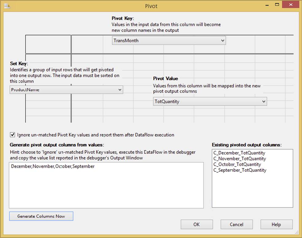
FIGURE 4-35
NOTE The output columns are generated in exactly the same order that they appear on the output columns collection.
13.To finish the example, add an OLE DB Destination. Configure to the AdventureWorks connection. Connect the Pivot Default Output to the input of the OLE DB Destination. Click the New button to alter the CREATE TABLE statement to build a table named PivotTable.
14.Add a Data Viewer in the pipe between the PIVOT and the OLE DB destination and run the package. You’ll see the data in a pivot table in the Data Viewer, as shown in the partial results in Figure 4-36.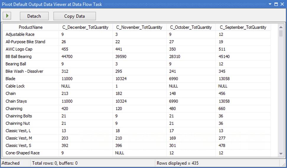
FIGURE 4-36
Unpivot
As you know, mainframe screens rarely conform to any normalized form. For example, a screen may show a Bill To Customer, a Ship To Customer, and a Dedicated To Customer field. Typically, the Data Source would store these three fields as three columns in a file (such as a virtual storage access system, or VSAM). Therefore, when you receive an extract from the mainframe you may have three columns, as shown in Figure 4-37.
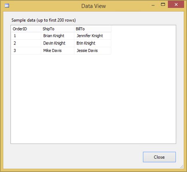
FIGURE 4-37
Your goal is to load this file into a Customer table in SQL Server. You want a row for each customer in each column, for a total of six rows in the Customer table, as shown in the CustomerName and OrderID columns in Figure 4-38.
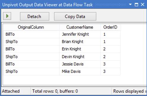
FIGURE 4-38
The Unpivot Transformation is a way to accomplish this business requirement. In this example, you’ll be shown how to use the Unpivot Transformation to create rows in the Data Flow from columns and shown how it is the opposite of the Pivot Transformation.
Your first step is to create a new package and drag a new Data Flow Task onto the Control Flow. From the Data Flow tab, configure the task. For this example, create a Flat File Connection Manager that points to UnPivotExample.csv, which looks like Figure 4-39 and can be downloaded from www.wrox.com/go/prossis2014. Name the Connection Manager FF Extract, and make the first row a header row. The file is comma-delimited, so you will want to specify the delimiter on the Columns page.
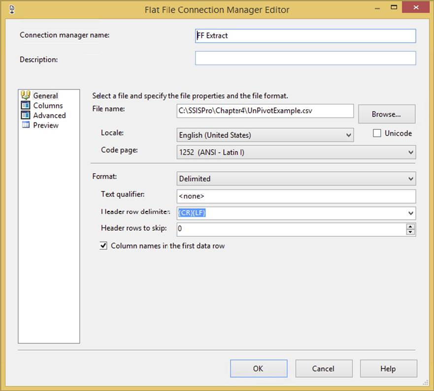
FIGURE 4-39
Once the Connection Manager is created, add a new Flat File Source and rename it “Mainframe Data.” Point the connection to the Pivot Source Connection Manager. Ensure that all the columns are checked in the Columns page on the source and click OK to go back to the Data Flow.
The next step is the most important step. You need to unpivot the data and make each column into a row in the Data Flow. You can do this by dragging an Unpivot Transformation onto the Data Flow and connecting it to the source. In this example, you want to unpivot the BillTo and ShipTo columns, and the OrderID column will just be passed through for each row. To do this, check each column you wish to unpivot, as shown in Figure 4-40, and check Pass Through for the OrderID column.
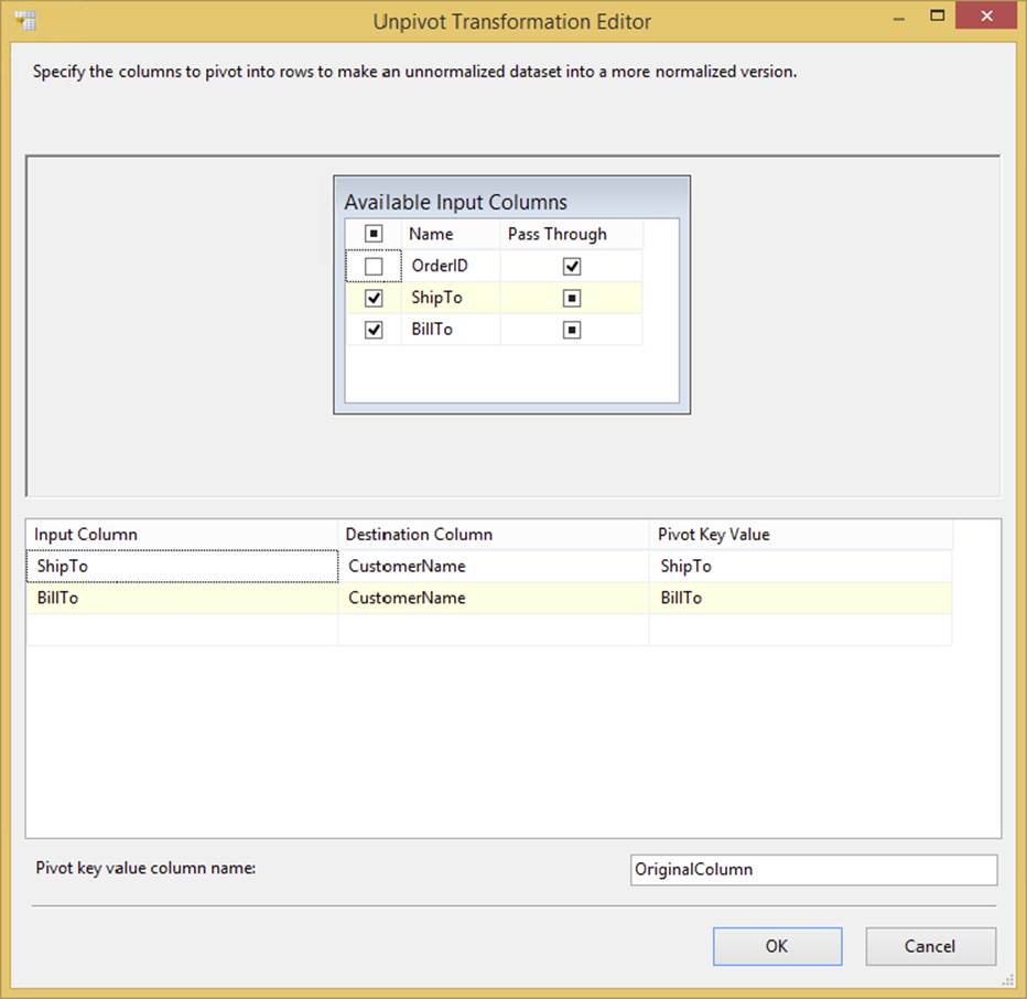
FIGURE 4-40
As you check each column that you wish to unpivot on, the column will be added to the grid below (shown in Figure 4-40). You’ll then need to type CustomerName for the Destination Column property for each row in the grid. This will write the data from each of the two columns into a single column called CustomerName. Optionally, you can also type Original Column for the Pivot Key Column Name property. By doing this, each row that’s written by the transformation will have an additional column called Original Column. This new column will state where the data came from.
The Pivot Transformation will take care of columns that have NULL values. For example, if your ShipTo column for OrderID 1 had a NULL value, that column will not be written as a row. You may wish to handle empty string values though, which will create blank rows in the Data Flow. To throw these records out, you can use a Conditional Split Transformation. In this transformation, you can create one condition for your good data that you wish to keep with the following code, which accepts only rows with actual data:
ISNULL(CustomerName) == FALSE && TRIM(CustomerName) != ""
The default (else) condition handles empty strings and NULL customers and in this example is called NULL Customer. After this, you’re ready to send the data to the destination of your choice. The simplest example is to send the data to a new SQL Server table in the AdventureWorks database.
Execute the package. You’ll see that the Valid Customer output goes to the customer table, and the NULL data condition is just thrown out. You could also place a data viewer prior to the OLE DB Destination to see the data interactively.
Term Extraction
If you have ever done some word and phrase analysis on websites for better search engine placement, you are familiar with the job that this transformation performs. The Term Extraction Transformation is a tool to mine free-flowing text for English word and phrase frequency. You can feed any text-based input stream into the transformation and it will output two columns: a text phrase and a statistical value for the phrase relative to the total input stream. The statistical values or scores that can be calculated can be as simple as a count of the frequency of the words and phrases, or they can be a little more complicated, such as the result of a formula named the TFIDF score. The TFIDF acronym stands for Term Frequency and Inverse Document Frequency, and it is a formula designed to balance the frequency of the distinct words and phrases relative to the total text sampled. If you’re interested, here’s the formula:
TDIDF (of term or phrase) = (frequency of term) * log((# rows in sample)/ (#
rows with term or phrase))
The results generated by the Term Extraction Transformation are based on internal algorithms and statistical models that are encapsulated in the component. You can’t alter or gain any insight into this logic by examining the code. However, some of the core rules about how the logic breaks apart the text to determine word and phrase boundaries are documented in Books Online. What you can do is tweak some external settings and make adjustments to the extraction behavior by examining the resulting output. Because text extraction is domain-specific, the transformation also provides the capability to store terms and phrases that you have predetermined are noisy or insignificant in your final results. You can then automatically remove these items from future extractions. Within just a few testing iterations, you can have the transformation producing meaningful results.
Before you write this transformation off as a cool utility that you’ll never use, consider this: How useful would it be to query into something like a customer service memo field stored in your data warehouse and generate some statistics about the comments being made? This is the type of usage for which the Term Extraction Transformation is perfectly suited. The trick to understanding how to use the component is to remember that it has one input. That input must be either a NULL-terminated ANSI (DT_WSTR) or a Unicode (DT_NTEXT) string. If your input stream is not one of these two types, you can use the Data Conversion Transformation to convert it. Because this transformation can best be learned by playing around with all the settings, the next example puts this transformation to work doing exactly what was proposed earlier — mining some customer service memo fields.
Assume you have a set of comment fields from a customer service database for an appliance manufacturer. In this field, the customer service representative records a note that summarizes his or her contact with the customer. For simplicity’s sake, you’ll create these comment fields in a text file and analyze them in the Term Extraction Transformation.
1. Create the customer service text file using the following text (you can download the code file custsvc.txt from www.wrox.com/go/prossis2014). Save it as c:\ProSSIS\Chapter4\custsvc.txt.
2. Ice maker in freezer stopped working model XX-YY3
3. Door to refrigerator is coming off model XX-1
4. Ice maker is making a funny noise XX-YY3
5. Handle on fridge falling off model XX-Z1
6. Freezer is not getting cold enough XX-1
7. Ice maker grinding sound fridge XX-YY3
8. Customer asking how to get the ice maker to work model XX-YY3
9. Customer complaining about dent in side panel model XX-Z1
10. Dent in model XX-Z1
11. Customer wants to exchange model XX-Z1 because of dent in door
Handle is wiggling model XX-Z1
12.Create a new SSIS package named TermExtractionExample. Add a Data Flow Task to the Control Flow design surface.
13.Create a Flat File connection to c:\ProSSIS\Chapter4\custsvc.txt. Uncheck “Column names in first data row”. Change the output column named in the Advanced tab to CustSvcNote. Change OutputColumnWidth to 100 to account for the length of the field. Change the data type to DT_WSTR.
14.Add a Flat File Source to the Data Flow design surface. Configure the source to use the Flat File connection.
15.Add a Term Extraction Transformation to the Data Flow design surface. Connect the output of the Flat File Source to its input. Open the Term Extraction Transformation Editor. Figure 4-41 shows the available input columns from the input stream and the two default-named output columns. You can change the named output columns if you wish. Only one input column can be chosen. Click the column CustSvcNote, as this is the column that is converted to a Unicode string. If you click the unconverted column, you’ll see a validation error like the following: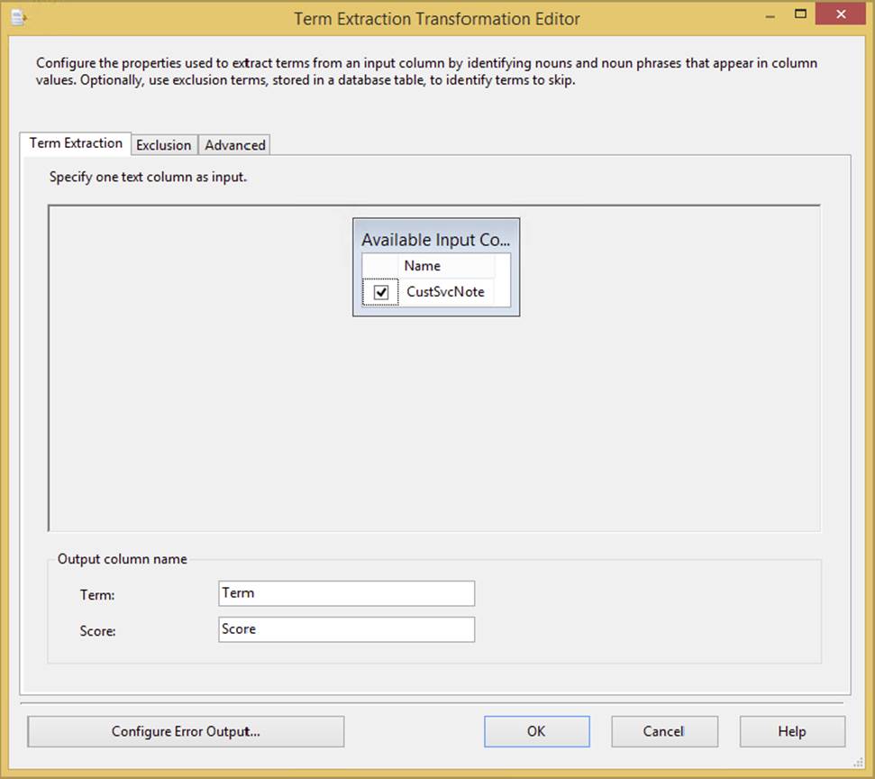
FIGURE 4-41
The input column can only have DT_WSTR or DT_NTEXT as its data type.
16.Even though we’re not going to set these tabs, the Exclusion tab enables you to specify noise words for the Term Extraction to ignore. The Advanced tab enables you to control how many times the word must appear before you output it as evidence. Close the Term Extraction Transformation Editor. Ignore the cautionary warnings about rows sent to error outputs. You didn’t configure an error location where bad rows should be saved, but it’s not necessary for this example.
17.Add an OLE DB Destination to the Data Flow. Connect the output of the Term Extraction Task to the OLE DB Destination. Configure the OLE DB Destination to use your AdventureWorks connection.
18.Click the New button to configure the Name of Table or View property. A window will come up with a CREATE TABLE DDL statement. Notice that the data types are a Unicode text field and a double. Alter the statement to read as follows:
19. CREATE TABLE TermResults (
20. [Term] NVARCHAR(128),
21. [Score] DOUBLE PRECISION
)
22.When you click OK, the new table TermResults will be created in the AdventureWorks database. Click the Mappings tab to confirm the mapping between the Term Extraction outputs of Term and Score to the table TermResults.
23.Add a data viewer by right-clicking the Data Flow between the Term Extraction Transformation and the OLE DB Destination. Set the type to grid and accept the defaults.
24.Run the package.
The package will stop on the data viewer that is shown in Figure 4-42 to enable you to view the results of the Term Extraction Transformation. You should see a list of terms and an associated score for each word. Because you accepted all of the Term Extraction settings, the default score is a simple count of frequency. Stop the package, open the Term Extraction Transformation Editor, and view the Advanced tab.
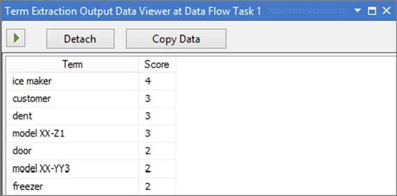
FIGURE 4-42
The Advanced tab, which allows for some configuration of the task, is divided into four categories:
· Term Type: Settings that control how the input stream should be broken into bits called tokens. The Noun Term Type focuses the transformation on nouns only, Noun Phrases extracts noun phrases, and Noun and Noun Phrases extracts both.
· Score Type: Choose to analyze words either by frequency or by a weighted frequency.
· Parameters: Frequency threshold is the minimum number of times a word or phrase must appear in tokens. Maximum length of term is the maximum number of words that should be combined together for evaluation.
· Options: Check this option to consider case sensitivity or leave it unchecked to disregard.
This is where the work really starts. How you set the transformation up greatly affects the results you’ll see. Figure 4-43 shows an example of the results using each of the different Term Type (noun) settings combined with the different score types [Tascam Digital Interface (TDIF)].
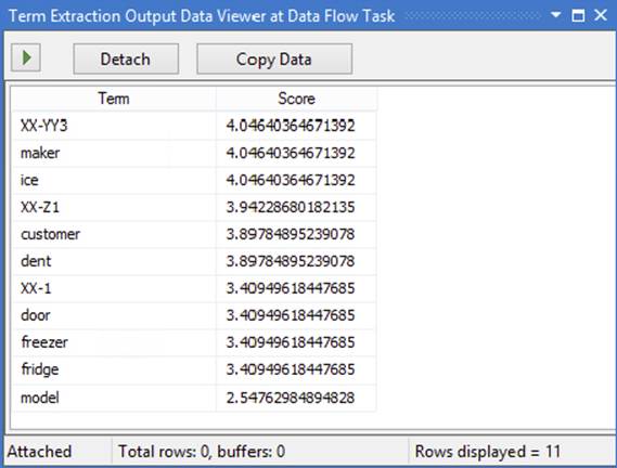
FIGURE 4-43
Currently, using a combination of these statistics, you can report that customer service is logging a high percentage of calls concerning the terms “model,” “model XX-Z1,” “model XX-YY3,” “ice maker,” “dent,” and “customer.” From this, one can assume that there may be some issues with models XX-Z1 and XX-YY3 that your client needs to look into.
In evaluating this data, you might determine that over time some words are just not relevant to the analysis. In this example, the words “model” and “customer” serve no purpose and only dampen the scores for other words. To remove these words from your analysis, take advantage of the exclusion features in the Term Extraction Transformation by adding these words to a table.
To really make sense of that word list, you need to add some human intervention and the next transformation — Term Lookup.
Term Lookup
The Term Lookup Transformation uses the same algorithms and statistical models as the Term Extraction Transformation to break up an incoming stream into noun or noun phrase tokens, but it is designed to compare those tokens to a stored word list and output a matching list of terms and phrases with simple frequency counts. Now a strategy for working with both term-based transformations should become clear. Periodically use the Term Extraction Transformation to mine the text data and generate lists of statistical phrases. Store these phrases in a word list, along with phrases that you think the term extraction process should identify. Remove any phrases that you don’t want identified. Use the Term Lookup Transformation to reprocess the text input to generate your final statistics. This way, you are generating statistics on known phrases of importance. A real-world application of this would be to pull out all the customer service notes that had a given set of terms or that mention a competitor’s name.
You can use results from the Term Extraction example by removing the word “model” from the [TermExclusions] table for future Term Extractions. You would then want to review all the terms stored in the [TermResults] table, sort them out, remove the duplicates, and add back terms that make sense to your subject matter experts reading the text. Because you want to generate some statistics about which model numbers are causing customer service calls but you don’t want to restrict your extractions to only occurrences of the model number in conjunction with the word “model,” remove phrases combining the word “model” and the model number. The final [TermResults] table looks like a dictionary, resembling something like the following:
term
--------
dent
door
freezer
ice
ice maker
maker
XX-1
XX-YY3
XX-Z1
Using a copy of the package you built in the Extraction example, exchange the Term Extraction Transformation for a Term Lookup Transformation and change the OLE DB Destination to output to a table [TermReport].
Open the Term Lookup Transformation Editor. It should look similar to Figure 4-44. In the Reference Table tab, change the Reference Table Name option to TermResults. In the Term Lookup tab, map the ConvCustSvrNote column to the Term column on the right. Check the ConvCustSvrNote as a pass-through column. Three basic tabs are used to set up this task (in the Term Lookup Transformation Editor):
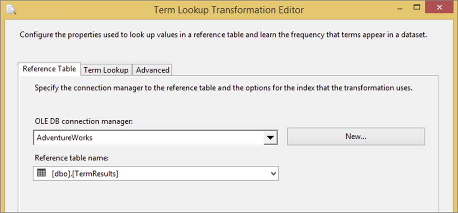
FIGURE 4-44
· Reference Table: This is where you configure the connection to the reference table. The Term Lookup Task should be used to validate each tokenized term that it finds in the input stream.
· Term Lookup: After selecting the lookup table, you map the field from the input stream to the reference table for matching.
· Advanced: This tab has one setting to check whether the matching is case sensitive.
The result of running this package is a list of phrases that you are expecting from your stored word list. A sample of the first six rows is displayed in the following code. Notice that this result set doesn’t summarize the findings. You are just given a blow-by-blow report on the number of terms in the word list that were found for each row of the customer service notes. In this text sample, it is just a coincidence that each term appears only once in each note.
term Frequency ConvCustSvcNote
----- --------- ------------------------------------------
freezer 1 ice maker in freezer stopped working model XX-YY3
ice maker 1 ice maker in freezer stopped working model XX-YY3
XX-YY3 1 ice maker in freezer stopped working model XX-YY3
Door 1 door to refrigerator is coming off model XX-1
XX-1 1 door to refrigerator is coming off model XX-1
ice maker 1 ice maker is making a funny noise XX-YY3
(Only first six rows of resultset are displayed)
To complete the report, you could add an Aggregate Transformation between the Term Lookup Transformation and the OLE DB Destination. Set up the Aggregate Transformation to ignore the ConvCustSvcNote column, group by the Term column, and summarize the Frequency Column. Connect the Aggregate Transformation to the OLE DB Destination and remap the columns in the OLE DB Destination.
Although this is a very rudimentary example, you can start to see the possibilities of using SSIS for very raw and unstructured Data Sources like this customer service comment data. In a short period of time, you have pulled some meaningful results from the data. Already you can provide the intelligence that model XX-Z1 is generating 45 percent of your sample calls and that 36 percent of your customer calls are related to the ice maker. Pretty cool results from what is considered unstructured data. This transformation is often used for advanced text mining.
DATA FLOW EXAMPLE
Now you can practice what you have learned in this chapter, pulling together some of the transformations and connections to create a small ETL process. This process will pull transactional data from the AdventureWorks database and then massage the data by aggregating, sorting, and calculating new columns. This extract may be used by another vendor or an internal organization.
Please note that this example uses a Sort and Aggregate Transformation. In reality it would be better to use T-SQL to replace that functionality.
1. Create a new package and rename it AdventureWorksExtract.dtsx. Start by dragging a Data Flow Task onto the Control Flow. Double-click the task to open the Data Flow tab.
2. In the Data Flow tab, drag an OLE DB Source onto the design pane. Right-click the source and rename it TransactionHistory. Double-click it to open the editor. Click the New button next to the OLE DB Connection Manager dropdown box. The connection to the AdventureWorks database may already be in the Data Connections list on the left. If it is, select it and click OK. Otherwise, click New to add a new connection to the AdventureWorks database on any server.
3. When you click OK, you’ll be taken back to the OLE DB Source Editor. Ensure that the Data Access Mode option is set to SQL Command. Type the following query for the command, as shown in Figure 4-45 or as follows: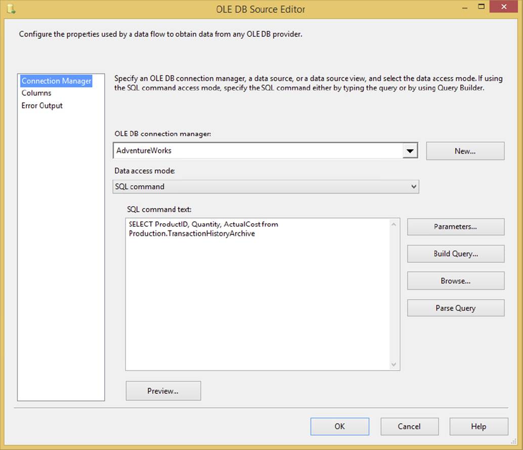
FIGURE 4-45
SELECT ProductID, Quantity, ActualCost from
Production.TransactionHistoryArchive
4. Drag a Derived Column Transformation onto the Data Flow, right-click it, and select Rename. Rename the transform Calculate Total Cost. Click the TransactionHistory OLE DB Source and drag the green arrow (the data path) onto the Derived Column Transformation.
5. Double-click the Derived Column Transformation to open the editor (shown in Figure 4-46). For the Expression column, type the following code or drag and drop the column names from the upper-left box: [Quantity]∗[ActualCost]. The Derived Column should have the <add as a new column> option selected, and type TotalCost for the Derived Column Name option. Click OK to exit the editor.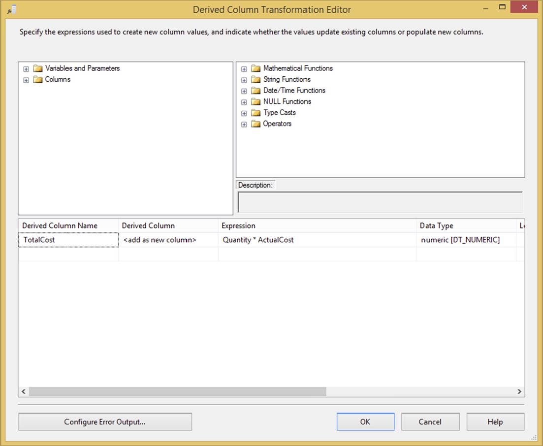
FIGURE 4-46
6. Drag an Aggregate Transformation onto the Data Flow and rename it Aggregate Data. Drag the blue arrow from the Derived Column Transformation onto this transformation. Double-click the Aggregate Transformation to open its editor (shown in Figure 4-47). Select the ProductID column and note that it is transposed into the bottom section. The ProductID column should have Group By for the Operation column. Next, check the Quantity and TotalCost columns and set the operation of both of these columns to Sum. Click OK to exit the editor.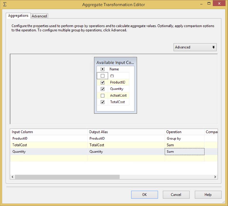
FIGURE 4-47
7. Drag a Sort Transformation onto the Data Flow and rename it Sort by Quantity. Connect the Aggregate Transformation to this transformation by the blue arrow as in the preceding step. Double-click the Sort Transformation to configure it in the editor. You can sort by the most popular products by checking the Quantity column and selecting Descending for the Sort Type dropdown box. Click OK to exit the editor.
8. You have now done enough massaging of the data and are ready to export the data to a flat file that can be consumed by another vendor. Drag a Flat File Destination onto the Data Flow. Connect it to the Sort Transformation by using the blue arrow as shown in the last few steps. Rename the Flat File Destination Vendor Extract.
9. Double-click the destination to open the Flat File Destination Editor. You’re going to output the data to a new Connection Manager, so click New. When prompted for the Flat File Format, select Delimited. Name the Connection Manager Vendor Extract also, and type whatever description you’d like. If you have the directory, point the File Name option to C:\ProSSIS\Chapter4\VendorExtract.csv (make sure this directory is created before proceeding). Check the “Column names in the first data row” option. Your final screen should look like Figure 4-48. Click OK to go back to the Flat File Destination Editor.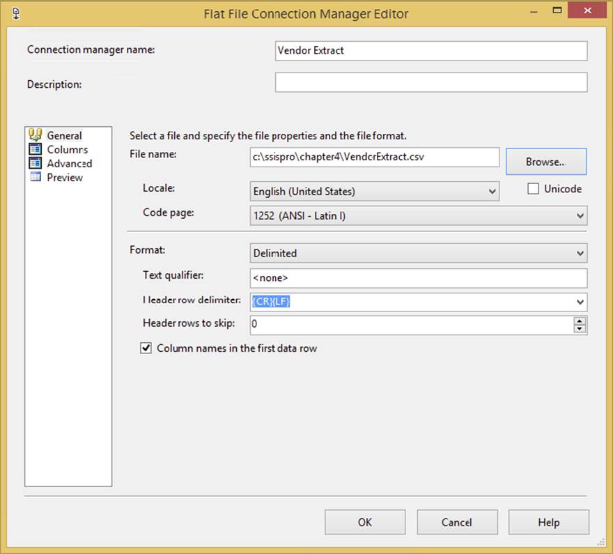
FIGURE 4-48
10.From the Mappings page, ensure that each column in the Inputs table is mapped to the Destination table. Click OK to exit the editor and go back to the Data Flow.
Now your first larger ETL package is complete! This package is very typical of what you’ll be doing daily inside of SSIS, and you will see this expanded on greatly, in Chapter 8. Execute the package. You should see the rows flow through the Data Flow, as shown inFigure 4-49. Note that as the data flows from transformation to transformation, you can see how many records were passed through.
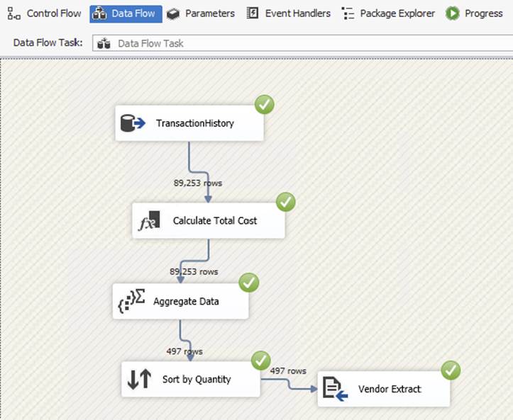
FIGURE 4-49
SUMMARY
The SSIS Data Flow moves data from a variety of sources and then transforms the data in memory prior to landing the data into a destination. Because it is in memory, it has superior speed to loading data into a table and performing a number of T-SQL transformations. In this chapter you learned about the common sources, destinations, and transformations used in the SSIS Data Flow. In the next chapter, you learn how to make SSIS dynamic by using variables and expressions.
All materials on the site are licensed Creative Commons Attribution-Sharealike 3.0 Unported CC BY-SA 3.0 & GNU Free Documentation License (GFDL)
If you are the copyright holder of any material contained on our site and intend to remove it, please contact our site administrator for approval.
© 2016-2026 All site design rights belong to S.Y.A.