MySQL Stored Procedure Programming (2009)
Part IV. Optimizing Stored Programs
Chapter 21. Advanced SQL Tuning
In the last chapter, we emphasized that high-performance stored programs require optimized SQL statements. We then reviewed the basic elements of SQL tuning — namely, how to optimize single-table accesses and simple joins. These operations form the building blocks for more complex SQL operations.
In this chapter, we will look at optimizing such SQL operations as:
§ Subqueries using the IN and EXISTS operators
§ "Anti-joins" using NOT IN or NOT EXISTS
§ "Unamed" views in FROM clauses
§ Named or permanent views
§ DML statements (INSERT, UPDATE, and DELETE)
Tuning Subqueries
A subquery is a SQL statement that is embedded within the WHERE clause of another statement. For instance, Example 21-1 uses a subquery to determine the number of customers who are also employees.
Example 21-1. SELECT statement with a subquery
SELECT COUNT(*)
FROM customers
WHERE (contact_surname, contact_firstname,date_of_birth)
IN (select surname,firstname,date_of_birth
FROM employees)
We can identify the subquery through the DEPENDENT SUBQUERY tag in the Select type column of the EXPLAIN statement output, as shown here:
Explain plan
------------
ID=1 Table=customers Select type=PRIMARY Access type=ALL
Rows=100459
Key= (Possible= )
Ref= Extra=Using where
ID=2 Table=employees Select type=DEPENDENT SUBQUERY Access type=ALL
Rows=1889
Key= (Possible= )
Ref= Extra=Using where
The same query can also be rewritten as an EXISTS subquery, as in Example 21-2.
Example 21-2. SELECT statement with an EXISTS subquery
SELECT count(*)
FROM customers
WHERE EXISTS (SELECT 'anything'
FROM employees
where surname=customers.contact_surname
AND firstname=customers.contact_firstname
AND date_of_birth=customers.date_of_birth)
Short Explain
-------------
1 PRIMARY select(ALL) on customers using no key
Using where
2 DEPENDENT SUBQUERY select(ALL) on employees using no key
Note that the EXPLAIN output for the EXISTS subquery is identical to that of the IN subquery. This is because MySQL rewrites IN-based subqueries as EXISTS-based syntax before execution. The performance of subqueries will, therefore, be the same, regardless of whether you use theEXISTS or the IN operator.
Optimizing Subqueries
When MySQL executes a statement that contains a subquery in the WHERE clause, it will execute the subquery once for every row returned by the main or "outer" SQL statement. It therefore follows that the subquery had better execute very efficiently: it is potentially going to be executed many times. The most obvious way to make a subquery run fast is to ensure that it is supported by an index. Ideally, we should create a concatenated index that includes every column referenced within the subquery.
For our example query in the previous example, we should create an index on all the employees columns referenced in the subquery:
CREATE INDEX i_customers_name ON customers
(contact_surname, contact_firstname, date_of_birth)
We can see from the following EXPLAIN output that MySQL makes use of the index to resolve the subquery. The output also includes the Using index clause, indicating that only the index is used—the most desirable execution plan for a subquery.
Short Explain
-------------
1 PRIMARY select(ALL) on employees using no key
Using where
2 DEPENDENT SUBQUERY select(index_subquery) on customers
using i_customers_name
Using index; Using where
Figure 21-1 shows the relative performance of both the EXISTS and IN subqueries with and without an index.
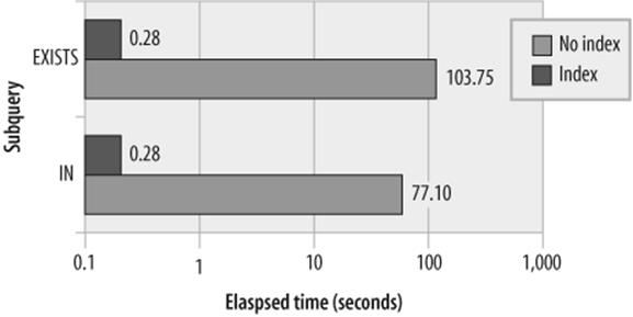
Figure 21-1. Subquery performance with and without an index
Not only will an indexed subquery outperform a nonindexed subquery, but the un-indexed subquery will also degrade exponentially as the number of rows in each of the tables increases. (The response time will actually be proportional to the number of rows returned by the outer query times the number of rows accessed in the subquery.) Figure 21-2 shows this exponential degradation.
Tip
Subqueries should be optimized by creating an index on all of the columns referenced in the subquery. SQL statements containing subqueries that are not supported by an index can show exponential degradation as table row counts increase.
Rewriting a Subquery as a Join
Many subqueries can be rewritten as joins. For instance, our example subquery could have been expressed as a join, as shown in Example 21-3.
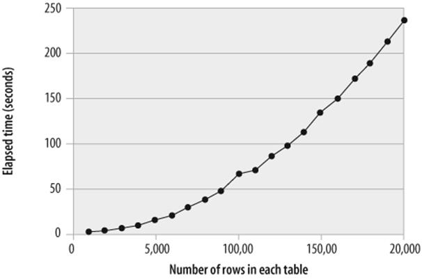
Figure 21-2. Exponential degradation in nonindexed subqueries
Example 21-3. Subquery rewritten as a join
SELECT count(*)
FROM customers JOIN employees
ON (employees.surname=customers.contact_surname
AND employees.firstname=customers.contact_firstname
AND employees.date_of_birth=customers.date_of_birth)
Subqueries sometimes result in queries that are easier to understand, and when the subquery is indexed, the performance of both types of subqueries and the join is virtually identical, although, as described in the previous section, EXISTS has a small advantage over IN. Figure 21-3 compares the three solutions for various sizes of tables.
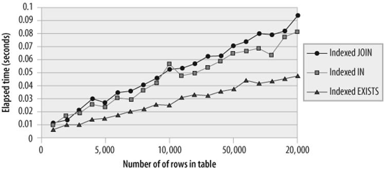
Figure 21-3. IN, EXISTS, and JOIN solution scalability (indexed query)
However, when no index exists to support the subquery or the join, then the join will outperform both IN and EXISTS subqueries. It will also degrade less rapidly as the number of rows to be processed increases. This is because of the MySQL join optimizations. Figure 21-4 shows the performance characteristics of the three solutions where no index exists.
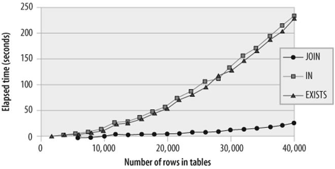
Figure 21-4. Comparison of nonindexed JOIN, IN, and EXISTS performance
Tip
A join will usually outperform an equivalent SQL with a subquery—and will show superior scalability—if there is no index to support either the join or the subquery. If there are supporting indexes, the performance differences among the three solutions are negligible.
Using Subqueries in Complex Joins
Although a subquery, in general, will not outperform an equivalent join, there are occasions when you can use subqueries to obtain more favorable execution plans for complex joins —especially when index merge operations are concerned.
Let's look at an example. You have an application that from time to time is asked to report on the quantity of sales made to a particular customer by a particular sales rep. The SQL might look like Example 21-4.
Example 21-4. Complex join SQL
SELECT COUNT(*), SUM(sales.quantity), SUM(sales.sale_value)
FROM sales
JOIN customers ON (sales.customer_id=customers.customer_id)
JOIN employees ON (sales.sales_rep_id=employees.employee_id)
JOIN products ON (sales.product_id=products.product_id)
WHERE customers.customer_name='INVITRO INTERNATIONAL'
AND employees.surname='GRIGSBY'
AND employees.firstname='RAY'
AND products.product_description='SLX';
We already have an index on the primary key columns for customers, employees, and products, so MySQL uses these indexes to join the appropriate rows from these tables to the sales table. In the process, it eliminates all of the rows except those that match the WHERE clause condition:
Short Explain
-------------
1 SIMPLE select(ALL) on sales using no key
1 SIMPLE select(eq_ref) on employees using PRIMARY
Using where
1 SIMPLE select(eq_ref) on customers using PRIMARY
Using where
1 SIMPLE select(eq_ref) on products using PRIMARY
Using where
This turns out to be a fairly expensive query, because we have to perform a full scan of the large sales table. What we probably want to do is to retrieve the appropriate primary keys from products, customers, and employees using the WHERE clause conditions, and then look up those keys (quickly) in the sales table. To allow us to quickly find these primary keys, we would create the following indexes:
CREATE INDEX i_customer_name ON customers(customer_name);
CREATE INDEX i_product_description ON products(product_description);
CREATE INDEX i_employee_name ON employees(surname, firstname);
To enable a rapid sales table lookup, we would create the following index:
CREATE INDEX i_sales_cust_prod_rep ON sales(customer_id,product_id,sales_rep_id);
Once we do this, our execution plan looks like this:
Short Explain
-------------
1 SIMPLE select(ref) on customers using i_customer_name
Using where; Using index
1 SIMPLE select(ref) on employees using i_employee_name
Using where; Using index
1 SIMPLE select(ref) on products using i_product_description
Using where; Using index
1 SIMPLE select(ref) on sales using i_sales_cust_prod_rep
Using where
Each step is now based on an index lookup, and the sales lookup is optimized through a fast concatenated index. The execution time reduces from about 25 seconds (almost half a minute) to about 0.01 second (almost instantaneous).
Tip
To optimize a join, create indexes to support all of the conditions in the WHERE clause and create concatenated indexes to support all of the join conditions.
As we noted in the previous chapter, we can't always create all of the concatenated indexes that we might need to support all possible queries on a table. In this case, we may want to perform an "index merge" of multiple single-column indexes. However, MySQL will not normally perform an index merge when optimizing a join.
In this case, to get an index merge join, we can try to rewrite the join using subqueries, as shown in Example 21-5.
Example 21-5. Complex join SQL rewritten to support index merge
SELECT COUNT(*), SUM(sales.quantity), SUM(sales.sale_value)
FROM sales
WHERE product_id= (SELECT product_id
FROM products
WHERE product_description='SLX')
AND sales_rep_id=(SELECT employee_id
FROM employees
WHERE surname='GRIGSBY'
AND firstname='RAY')
AND customer_id= (SELECT customer_id
FROM customers
WHERE customer_name='INVITRO INTERNATIONAL');
The EXPLAIN output shows that an index merge will now occur, as shown in Example 21-6.
Example 21-6. EXPLAIN output for an index merge SQL
Short Explain
-------------
1 PRIMARY select(index_merge) on sales using i_sales_rep,i_sales_cust
Using intersect(i_sales_rep,i_sales_cust); Using where
4 SUBQUERY select(ref) on customers using i_customer_name
3 SUBQUERY select(ref) on employees using i_employee_name
2 SUBQUERY select(ref) on products using i_product_description
The performance of the index merge solution is about 0.025 second—slower than the concatenated index but still about 1,000 times faster than the initial join performance. This is an especially useful technique if you have a STAR schema (one very large table that contains the "facts," with foreign keys pointing to other, smaller "dimension" tables).
Figure 21-5 compares the performance of the three approaches. Although an index merge is not quite as efficient as a concatenated index, you can often satisfy a wider range of queries using an index merge, since this way you need only create indexes on each column, not concatenated indexes on every possible combination of columns.
Tip
Rewriting a join with subqueries can improve join performance, especially if you need to perform an index merge join—consider this technique for STAR joins.
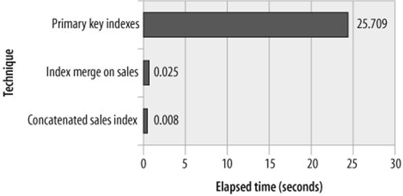
Figure 21-5. Optimizing a complex join with subqueries and index merge
Tuning "Anti-Joins" Using Subqueries
With an anti-join, we retrieve all rows from one table for which there is no matching row in another table. There are a number of ways of expressing anti-joins in MySQL.
Perhaps the most natural way of writing an anti-join is to express it as a NOT IN subquery. For instance, Example 21-7 returns all of the customers who are not employees.
Example 21-7. Example of an anti-join using NOT IN
SELECT count(*)
FROM customers
WHERE (contact_surname,contact_firstname, date_of_birth)
NOT IN (SELECT surname,firstname, date_of_birth
FROM employees)
Short Explain
-------------
1 PRIMARY select(ALL) on customers using no key
Using where
2 DEPENDENT SUBQUERY select(ALL) on employees using no key
Using where
Another way to express this query is to use a NOT EXISTS subquery. Just as MySQL will rewrite IN subqueries to use the EXISTS clause, so too will MySQL rewrite a NOT IN subquery as a NOT EXISTS. So, from MySQL's perspective, Example 21-7 and Example 21-8 are equivalent.
Example 21-8. Example of an anti-join using NOT EXISTS
SELECT count(*)
FROM customers
WHERE NOT EXISTS (SELECT *
FROM employees
WHERE surname=customers.contact_surname
AND firstname=customers.contact_firstname
AND date_of_birth=customers.date_of_birth)
Short Explain
-------------
1 PRIMARY select(ALL) on customers using no key
Using where
2 DEPENDENT SUBQUERY select(ALL) on employees using no key
Using where
A third but somewhat less natural way to express this query is to use a LEFT JOIN. This is a join in which all rows from the first table are returned even if there is no matching row in the second table. NULLs are returned for columns from the second table that do not have a matching row.
In Example 21-9 we join customers to employees and return NULL values for all of the employees who are not also customers. We can use this characteristic to eliminate the customers who are not also employees by testing for a NULL in a normally NOT NULL customer column.
Example 21-9. Example of an anti-join using LEFT JOIN
SELECT count(*)
FROM customers
LEFT JOIN employees
ON (customers.contact_surname=employees.surname
and customers.contact_firstname=employees.firstname
and customers.date_of_birth=employees.date_of_birth)
WHERE employees.surname IS NULL
Short Explain
-------------
1 SIMPLE select(ALL) on customers using no key
1 SIMPLE select(ALL) on employees using no key
Using where; Not exists
Optimizing an Anti-Join
The guidelines for optimizing anti-joins using subqueries or left joins are identical to the guidelines for optimizing normal subqueries or joins. Scalability and good performance will be achieved only if we create an index to optimize the subquery or the join. For the previous examples, this would mean creating an index on customer names as follows:[*]
CREATE INDEX i_customers_name ON employees(surname,firstname,date_of_birth);
Figure 21-6 shows the massive performance improvements that result when we create a supporting index for an anti-join.
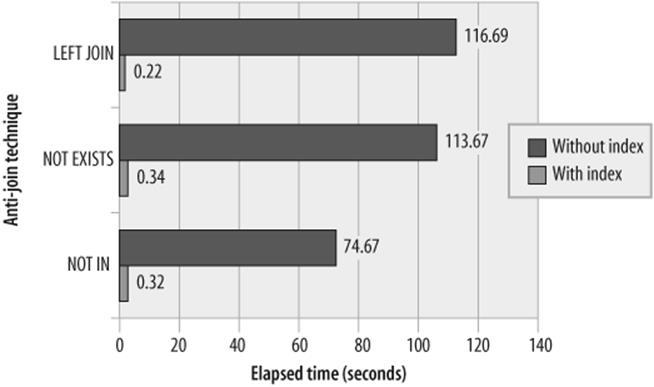
Figure 21-6. Comparison of anti-join techniques
Figure 21-6 also shows a substantial performance advantage for the NOT IN subquery over NOT EXISTS or LEFT JOIN when there is no index to support the anti-join. We noted earlier that MySQL rewrites the NOT IN-based statement to a NOT EXISTS, so it is at first surprising that there should be a performance difference. However, examination of the NOT IN rewrite reveals a number of undocumented compiler directives within the rewritten SQL that appear to give NOT IN a substantial performance advantage in the absence of an index.
Not only is the LEFT JOIN technique slower than NOT IN or NOT EXISTS, but it degrades much faster as the quantity of data to be processed increases. Figure 21-7 shows that the LEFT JOIN version of the anti-join degrades much more rapidly as the size of the tables being joined increases—this is the opposite of the effect shown for normal subqueries, where the join solution was found to be more scalable than the subquery solution (refer to Figure 21-3).
Tip
To optimize an anti-join, create indexes to support the subquery or right hand table of a LEFT JOIN. If you cannot support the subquery with an index, use NOT IN in preference to NOT EXISTS or LEFT JOIN.
[*] It might occur to you that creating an index on customers would produce a better join than the index on employees. However, LEFT JOINs can only be performed with the table that will return all rows as the first table in the join—this means that the join order can only be customersto employees, and therefore the index to support the join must be on employees.
Tuning Subqueries in the FROM Clause
It is possible to include subqueries within the FROM clause of a SQL statement. Such subqueries are sometimes called unnamed views , derived tables , or inline views .
For instance, consider the query in Example 21-10, which retrieves a list of employees and department details for employees older than 55 years.
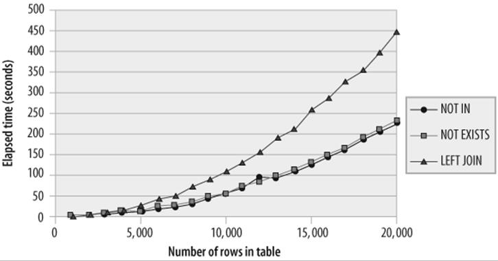
Figure 21-7. Scalability of various anti-join techniques (no index)
Example 21-10. Example SQL suitable for rewrite with an inline view
SELECT departments.department_name,employee_id,surname,firstname
FROM departments
JOIN employees
USING (department_id)
WHERE employees.date_of_birth<date_sub(curdate( ),interval 55 year)
Short Explain
1 SIMPLE select(range) on employees using i_employee_dob
Using where
1 SIMPLE select(eq_ref) on departments using PRIMARY
Using where
This query is well optimized—an index on date of birth finds the customers, and the primary key index is used to find the department name on the departments table. However, we could write this query using inline views in the FROM clause, as shown in Example 21-11.
Example 21-11. SQL rewritten with an inline view
SELECT departments.department_name,employee_id,surname,firstname
FROM (SELECT * FROM departments ) departments
JOIN (SELECT * FROM employees) employees
USING (department_id)
WHERE employees.date_of_birth<DATE_SUB(curdate( ), INTERVAL 55 YEAR)
Explain plan
1 PRIMARY select(ALL) on <derived2> using no key
1 PRIMARY select(ALL) on <derived3> using no key
Using where
3 DERIVED select(ALL) on employees using no key
2 DERIVED select(ALL) on departments using no key
This execution plan is somewhat different from those we have looked at in previous examples, and it warrants some explanation. The first two steps indicate that a join was performed between two "derived" tables—our subqueries inside the FROM clause. The next two steps show how each of the derived tables was created. Note that the name of the table—<derived2>, for instance—indicates the ID of the step that created it. So we can see from the plan that <derived2> was created from a full table scan of departments.
Derived tables are effectively temporary tables created by executing the SQL inside the subquery. You can imagine that something like the following SQL is being executed to create the <derived2> table:
CREATE TEMPORARY TABLE derived2 AS
SELECT * FROM departments
Simply by using subqueries in the FROM clause, we have substantially weakened MySQL's chances of implementing an efficient join. MySQL must first execute the subqueries' statements to create the derived tables and then join those two derived tables. Derived tables have no indexes, so this particular rewrite could not take advantage of the indexes that were so effective in our original query (shown in Example 21-10). In this case, both the index to support the WHERE clause and the index supporting the join were unusable.
We could improve the query by moving the WHERE clause condition on employees into the subquery, as shown in Example 21-12.
Example 21-12. Rewritten SQL using an inline view
SELECT departments.department_name,employee_id,surname,firstname
FROM (SELECT * FROM departments ) departments
JOIN (SELECT * FROM employees
WHERE employees.date_of_birth
<DATE_SUB(curdate( ),INTERVAL 55 YEAR)) employees
USING (department_id)
Explain plan
------------
1 PRIMARY select(system) on <derived3> using no key
1 PRIMARY select(ALL) on <derived2> using no key
Using where
3 DERIVED select(range) on employees using i_employee_dob
Using where
4 DERIVED select(ALL) on departments using no key
This plan at least allows us to use an index to find the relevant customers, but still prevents the use of an index to join those rows to the appropriate department.
Tip
In general, avoid using derived tables (subqueries in the FROM clause), because the resulting temporary tables have no indexes and cannot be effectively joined or searched. If you must use derived tables, try to move all WHERE clause conditions inside of the subqueries.
Using Views
A view can be thought of as a "stored query". A view definition essentially creates a named definition for a SQL statement that can then be referenced as a table in other SQL statements. For instance, we could create a view on the sales table that returns only sales for the year 2004, as shown in Example 21-13.
Example 21-13. View to return sales table data for 2004
CREATE OR REPLACE VIEW v_sales_2004
(sales_id,customer_id,product_id,sale_date,
quantity,sale_value,department_id,sales_rep_id,gst_flag) AS
SELECT sales_id,customer_id,product_id,sale_date,
quantity,sale_value,department_id,sales_rep_id,gst_flag
FROM sales
WHERE sale_date BETWEEN '2004-01-01' AND '2004-12-31'
The CREATE VIEW syntax includes an ALGORITHM clause, which defines how the view will be processed at runtime:
CREATE [ALGORITHM = {UNDEFINED | MERGE
| TEMPTABLE}] VIEWviewname
The view algorithm may be set to one of the following:
TEMPTABLE
MySQL will process the view in very much the same way as a derived table—it will create a temporary table using the SQL associated with the view, and then use that temporary table wherever the view name is referenced in the original query.
MERGE
MySQL will attempt to merge the view SQL into the original query in an efficient manner.
UNDEFINED
Allows MySQL to choose the algorithm, which results in MySQL using the MERGE technique when possible.
Because the TEMPTABLE algorithm uses temporary tables—which will not have associated indexes—its performance will often be inferior to native SQL or to SQL that uses a view defined with the MERGE algorithm.
Consider the SQL query shown in Example 21-14; it uses the view definition from Example 21-13 and adds some additional WHERE clause conditions. The view WHERE clause, as well as the additional WHERE clauses in the SQL, is supported by the index i_sales_date_prod_cust, which includes the columns customer_id, product_id, and sale_date.
Example 21-14. SQL statement that references a view
SELECT SUM(quantity),SUM(sale_value)
FROM v_sales_2004_merge
WHERE customer_id=1
AND product_id=1;
This query could have been written in standard SQL, as shown in Example 21-15.
Example 21-15. Equivalent SQL statement without a view
SELECT SUM(quantity),SUM(sale_value)
FROM sales
WHERE sale_date BETWEEN '2004-01-01' and '2004-12-31'
AND customer_id=1
AND product_id=1
Alternately, we could have written the SQL using a derived table approach, as shown in Example 21-16.
Example 21-16. Equivalent SQL statement using derived tables
SELECT SUM(quantity),SUM(sale_value)
from (SELECT *
FROM sales
WHERE sale_date BETWEEN '2004-01-01' AND '2004-12-31') sales
WHERE customer_id=1
AND product_id=1;
We now have four ways to resolve the query—using a MERGE algorithm view, using a TEMPTABLE view, using a derived table, and using a plain old SQL statement. So which approach will result in the best performance?
Based on our understanding of the TEMPTABLE and MERGE algorithms, we would predict that a MERGE view would behave very similarly to the plain old SQL statement, while the TEMPTABLE algorithm would behave similarly to the derived table approach. Furthermore, we would predict that neither the TEMPTABLE nor the derived table approach would be able to leverage our index on product_id, customer_id, and sale_date, and so both will be substantially slower.
Our predictions were confirmed. The SQLs that used the TEMPTABLE and the derived table approaches generated very similar EXPLAIN output, as shown in Example 21-17. In each case, MySQL performed a full scan of the sales table in order to create a temporary "derived" table containing data for 2004 only, and then performed a full scan of that derived table to retrieve rows for the appropriate product and customer.
Example 21-17. Execution plan for the derived table and TEMPTABLE view approaches
Short Explain
-------------
1 PRIMARY select(ALL) on <derived2> using no key
Using where
2 DERIVED select(ALL) on sales using no key
Using where
An EXPLAIN EXTENDED revealed that the MERGE view approach resulted in a rewrite against the sales table, as shown in Example 21-18.
Example 21-18. How MySQL rewrote the SQL to "merge" the view definition
SELECT sum('prod'.'sales'.'QUANTITY') AS 'SUM(quantity)',
sum('prod'.'sales'.'SALE_VALUE') AS 'SUM(sale_value)'
FROM 'prod'.'sales'
WHERE (('prod'.'sales'.'CUSTOMER_ID' = 1)
AND ('prod'.'sales'.'PRODUCT_ID' = 1)
AND ('prod'.'sales'.'SALE_DATE' between 20040101000000 and 20041231000000))
Short Explain
-------------
1 PRIMARY select(range) on sales using i_sales_cust_prod_date
Using where
Figure 21-8 shows the performance of the four approaches. As expected, the MERGE view gave equivalent performance to native SQL and was superior to both the TEMPTABLE and the derived table approaches.
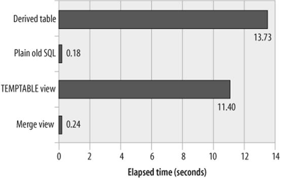
Figure 21-8. Comparison of view algorithm performance
Not all views can be resolved by a MERGE algorithm. In particular, views that include GROUP BY or other aggregate conditions (DISTINCT, SUM, etc.) must be resolved through a temporary table. It is also possible that in some cases the "merged" SQL generated by MySQL might be hard to optimize and that a temporary table approach might lead to better performance.
Tip
Views created with the TEMPTABLE algorithm may be unable to take advantage of indexes that are available to views created with the MERGE algorithm. Avoid using views that employ the TEMPTABLE algorithm unless you find that the "merged" SQL cannot be effectively optimized.
Tuning ORDER and GROUP BY
GROUP BY, ORDER BY, and certain group functions (MAX, MIN, etc.) may require that data be sorted before being returned to the user. You can detect that a sort is required from the Using filesort tag in the Extra column of the EXPLAIN statement output, as shown in Example 21-19.
Example 21-19. Simple SQL that performs a sort
SELECT *
FROM customers
ORDER BY contact_surname, contact_firstname
Explain plan
------------
ID=1 Table=customers Select type=SIMPLE Access type=ALL
Rows=101999
Key= (Possible= )
Ref= Extra=Using filesort
If there is sufficient memory, the sort can be performed without having to write intermediate results to disk. However, without sufficient memory, the overhead of the disk-based sort will often dominate the overall performance of the query.
There are two ways to avoid a disk-based sort:
§ Create an index on the columns to be sorted. MySQL can then use the index to retrieve the rows in sorted order.
§ Allocate more memory to the sort.
These approaches are described in the following sections.
Creating an Index to Avoid a Sort
If an index exists on the columns to be sorted, MySQL can use the index to avoid a sort. For instance, suppose that the following index exists:
CREATE INDEX i_customer_name ON customers(contact_surname, contact_firstname)
MYSQL can use that index to avoid the sort operation shown in Example 21-19. Example 21-20 shows the output when the index exists; note the absence of the Using filesort tag and that the i_customer_name index is used, even though there are no WHERE clause conditions that would suggest that the index was necessary.
Example 21-20. Using an index to avoid a sort
SELECT * from customers
ORDER BY contact_surname, contact_firstname
Explain plan
------------
ID=1 Table=customers Select type=SIMPLE
Access type=index Rows=101489
Key=i_customer_name (Possible= )
Ref= Extra=
Reducing Sort Overhead by Increasing Sort Memory
When MySQL performs a sort, it first sorts rows within an area of memory defined by the parameter SORT_BUFFER_SIZE. If the memory is exhausted, it writes the contents of the buffer to disk and reads more data into the buffer. This process is continued until all the rows are processed; then, the contents of the disk files are merged and the sorted results are returned to the query. The larger the size of the sort buffer, the fewer the disk files that need to be created and then merged. If the sort buffer is large enough, then the sort can complete entirely in memory.
You can allocate more memory to the sort by issuing a SET SORT_BUFFER_SIZE statement. For instance, the following allocates 10,485,760 bytes (10M) to the sort:
SET SORT_BUFFER_SIZE=10485760;
You can determine the current value of SORT_BUFFER_SIZE by issuing the following statement:
SHOW VARIABLES LIKE 'sort_buffer_size';
As you allocate more memory to the sort, performance will initially improve up to the point at which the sort can complete within a single "merge run." After that point, adding more memory appears to have no effect, until the point at which the sort can complete entirely in memory. After this point, adding more memory will not further improve sort performance. Figure 21-9 shows where these two plateaus of improvement occurred for the example above. It also shows the effect of creating an index to avoid the sort altogether.
To find out how many sort merge runs were required to process our SQL, we can examine the value for the status variable SORT_MERGE_PASSES from the SHOW STATUS statement before and after our SQL executes.
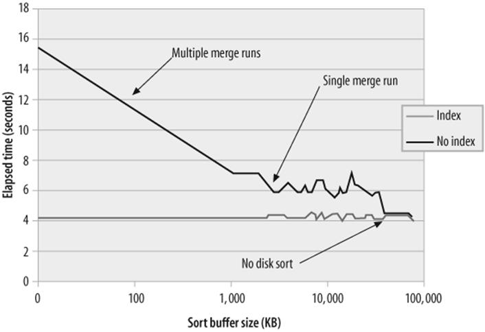
Figure 21-9. Optimizing ORDER BY through increasing sort buffer size or creating an index
Tip
To optimize SQL that must perform a sort (ORDER BY, GROUP BY), consider increasing the value of SORT_BUFFER_SIZE or create an index on the columns being sorted.
Tuning DML (INSERT, UPDATE, DELETE)
The first principle for optimizing UPDATE, DELETE, and INSERT statements is to optimize any WHERE clause conditions used to find the rows to be manipulated or inserted. The DELETE and UPDATE statements may contain WHERE clauses, and the INSERT statement may contain SQL that defines the data to be inserted. Ensure that these WHERE clauses are efficient—perhaps by creating appropriate concatenated indexes .
The second principle for optimizing DML performance is to avoid creating too many indexes. Whenever a row is inserted or deleted, updates must occur to every index that exists against the table. These indexes exist to improve query performance, but bear in mind that each index also results in overhead when the row is created or deleted. For updates, only the indexes that reference the specific columns being modified need to be updated.
Batching Inserts
The MySQL language allows more than one row to be inserted in a single INSERT operation. For instance, the statement in Example 21-21 inserts five rows into the clickstream_log table in a single call.
Example 21-21. Batch INSERT statement
INSERT INTO clickstream_log (url,timestamp,source_ip)
values
('http://dev.mysql.com/downloads/mysql/5.0.html',
'2005-02-10 11:46:23','192.168.34.87') ,
('http://dev.mysql.com/downloads/mysql/4.1.html',
'2005-02-10 11:46:24','192.168.35.78'),
('http://dev.mysql.com',
'2005-02-10 11:46:24','192.168.35.90'),
('http://www.mysql.com/bugs',
'2005-02-10 11:46:25','192.168.36.07'),
('http://dev.mysql.com/downloads/mysql/5.1.html',
'2005-02-10 11:46:25','192.168.36.12')
Batching INSERT operations in this way can radically improve performance. Figure 21-10 shows how the time taken to insert 10,000 rows into the table decreases as we increase the number of rows included within each INSERT statement. Inserting one row at a time, it took about 384 seconds to insert the rows. When inserting 100 rows at a time, we were able to add the same number of rows in only 7 seconds.
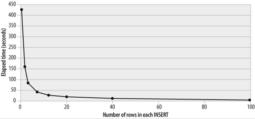
Figure 21-10. Performance improvement from multirow inserts
Tip
Whenever possible, use MySQL's multirow insert feature to speed up the bulk loading of records.
Optimizing DML by Reducing Commit Frequency
If we are using a transactional storage engine—for instance, if our tables are using the InnoDB engine—we should make sure that we are committing changes to the database only when necessary. Excessive commits will degrade performance.
By default, MySQL will issue an implicit commit after every SQL statement. When a commit occurs, a storage engine like InnoDB will write a record to its transaction log on disk to ensure that the transaction is persistent (i.e., to ensure that the transaction will not be lost if MySQL or our program crashes). These transaction log writes involve a physical I/O to the disk and therefore always add to our response time.
We can prevent this automatic commit behavior by issuing the SET AUTOCOMMIT=0 statement and/or by issuing a START TRANSACTION statement before issuing our statements. We can then issue a COMMIT statement at regular intervals, reducing the number of writes to the transaction log that will be required. (Note, though, that MySQL will occasionally write to the transaction log anyway when memory buffers require flushing.)
Usually, the frequency with which we commit is driven by our application logic rather than by performance. For instance, if a user clicks a Save button in our application, he is going to expect that the information will be permanently saved to the database, and so we will be required to issue aCOMMIT as a result. However, in batch applications, we can often choose to commit at relatively infrequent intervals. Reducing the commit frequency can have a huge effect on DML performance.
In Figure 21-11, we see how reducing the commit frequency affected the time taken to insert 10,000 rows into the database. At the default settings, it took about 850 seconds (about 14 minutes) to insert the 10,000 rows. If we commit only after every 100 rows have been inserted, the time taken is reduced to only 8 seconds.
In these tests, the InnoDB transaction log was on the same disk as the InnoDB tablespace files, which magnified the degradation caused by transaction log writes. Moving the transaction log to a dedicated disk can reduce—although not eliminate—the transaction log overhead.
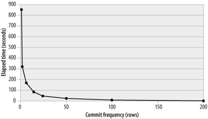
Figure 21-11. How commit frequency affects DML performance
Tip
When you are using a transactional storage engine (such as InnoDB) in situations where your application logic permits (batch applications, for instance), reducing the frequency at which you commit work can massively improve the performance of INSERTs, UPDATEs, andDELETEs.
We looked at how you can manipulate commit frequency in stored programs in Chapter 8.
Triggers and DML Performance
Because trigger code will be invoked for every row affected by the relevant DML operation, poorly performing triggers can have a very significant effect on DML performance . If our DML performance is a concern and there are triggers on the tables involved, we may want to determine the overhead of our triggers by measuring performance with and without the triggers.
We provide some more advice on trigger tuning in Chapter 22.
Conclusion
In this chapter, we looked at some more advanced SQL tuning scenarios.
We first looked at simple subqueries using the IN and EXISTS operators. As with joins and simple single-table queries, the most important factor in improving subquery performance is to create indexes that allow the subqueries to execute quickly. We also saw that when an appropriate index is not available, rewriting the subquery as a join can significantly improve performance.
The anti-join is a type of SQL operation that returns all rows from a table that do not have a matching row in a second table. These can be performed using NOT IN, NOT EXISTS, or LEFT JOIN operations. As with other subqueries, creating an index to support the subquery is the most important optimization. If no index exists to support the anti-join, then a NOT IN subquery will be more efficient than a NOT EXISTS or a LEFT JOIN.
We can also place subqueries in the FROM clause—these are sometimes referred to as inline views, unnamed views, or derived tables. Generally speaking, we should avoid this practice because the resulting "derived" tables will have no indexes and will perform poorly if they are joined to another table or if there are associated selection criteria in the WHERE clause. Named views are a much better option, since MySQL can "merge" the view definition into the calling query, which will allow the use of indexes if appropriate. However, views created with the TEMPTABLE option, or views that cannot take advantage of the MERGE algorithm (such as GROUP BY views), will exhibit similar performance to derived table queries.
When our SQL has an ORDER BY or GROUP BY condition, MySQL might need to sort the resulting data. We can tell if there has been a sort by the Using filesort tag in the Extra column of the EXPLAIN statement output. Large sorts can have a diabolical effect on our query performance, although we can improve performance by increasing the amount of memory available to the sort (by increasing SORT_BUFFER_SIZE). Alternately, we can create an index on the columns to be sorted. MySQL can then use that index to avoid the sort and thus improve performance.
We can achieve substantial improvements in performance by inserting multiple rows with each INSERT statement. If we are using a transactional storage engine such as InnoDB, we can improve the performance of any DML operations by reducing the frequency with which we commit data. However, we should never modify commit frequency at the expense of transactional integrity.
Most of our stored programs will perform only as well as the SQL that they contain. In the next chapter we will look at how to go the "last mile" by tuning the stored program code itself.
All materials on the site are licensed Creative Commons Attribution-Sharealike 3.0 Unported CC BY-SA 3.0 & GNU Free Documentation License (GFDL)
If you are the copyright holder of any material contained on our site and intend to remove it, please contact our site administrator for approval.
© 2016-2026 All site design rights belong to S.Y.A.