Foundations of Coding: Compression, Encryption, Error Correction (2015)
Chapter 2. Information Theory and Compression
2.2 Statistical Encoding
Statistical encoding schemes use the frequency of each character of the source for compression and, by encoding the most frequent characters with the shortest codewords, put themselves close to the entropy.
2.2.1 Huffman's Algorithm
These schemes enable one to find the best encoding for a source without memory ![]() . The code alphabet is V of size q. For the optimal nature of the result, one must check that
. The code alphabet is V of size q. For the optimal nature of the result, one must check that ![]() divides
divides ![]() (in order to obtain a locally complete tree). Otherwise, one can easily add some symbols in S, with probability of occurrence equal to zero, until
(in order to obtain a locally complete tree). Otherwise, one can easily add some symbols in S, with probability of occurrence equal to zero, until ![]() divides
divides ![]() . The related codewords (the longest ones) will not be used.
. The related codewords (the longest ones) will not be used.
|
Algorithm 2.1 Description of Huffman's Algorithm |
|
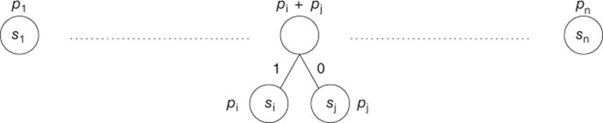
Using the source alphabet S, one builds a set of isolated nodes associated to the probabilities of |
|
Figure 2.1 Huffman encoding: beginning of the algorithm |
|
Let |
|
Figure 2.2 Huffman's encoding: first step ( |
|
One then restarts with the q lowest values among the nodes of highest level (the roots), until one obtains a single tree (at each step, the number of nodes of highest level is decreased by |

The idea of the method is given in Algorithm 2.1.
Example
Source Coding
One wishes to encode the following source over ![]() :
:
The successive steps of the algorithm are given in Figure 2.3.
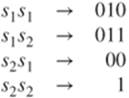
Then, one builds the following Huffman code:
Exercise 2.3 This exercise introduces some theoretical elements concerning the efficiency of the code generated by the Huffman algorithm. Let ![]() be the source with
be the source with ![]() , and
, and ![]() .
.
1. Compute the entropy of ![]() .
.
2. Give the code generated by the Huffman algorithm over the third extension ![]() . What is its compression rate?
. What is its compression rate?
3. What can you say about the efficiency of the Huffman algorithm when comparing the compression rates obtained here with those of Exercise 1.33? Does it comply with Shannon's theorem?
Solution on page 295.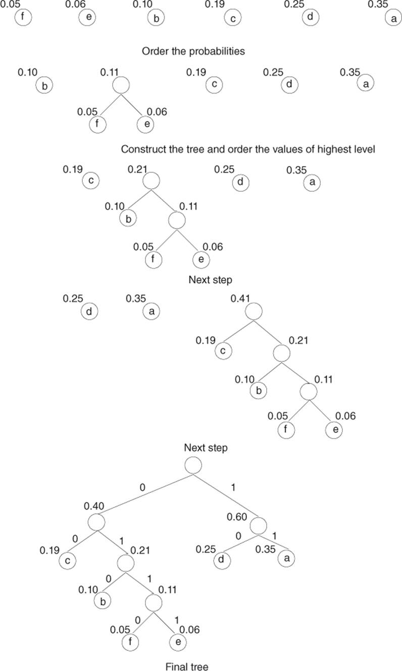
Figure 2.3 Example of a construction of the Huffman code
Exercise 2.4 (Heads or Tails to Play 421 Game)
One wishes to play with a die, while having only a coin. Therefore, the exercise concerns encoding a six-face fair die with a two-face fair coin.
1. What is the entropy of a die?
2. 2. Propose an encoding algorithm.
3. Compute the average length of this code.
4. Is this encoding optimal?
Solution on page 296.
2.2.1.1 Huffman's Algorithm is Optimal
23
Theorem 23
A code generated by the Huffman algorithm is optimal among all instantaneous codes in ![]() over V.
over V.
Proof
In order to simplify the notation in this proof, we suppose that ![]() . However, the results can be generalized at each step.
. However, the results can be generalized at each step.
One knows that an instantaneous code can be represented with the Huffman tree. Let A be the tree representing an optimal code, and let H be the tree representing a code generated by the Huffman algorithm.
One notices that in A, there does not exists a node with a single child whose leaves contain codewords (indeed, such a node can be replaced with its child in order to obtain a better code).
Moreover, if the respective probabilities of occurrence ![]() for two codewords
for two codewords ![]() in A satisfy
in A satisfy ![]() , then the respective depth of the leaves representing
, then the respective depth of the leaves representing ![]() —satisfy
—satisfy ![]() (indeed, otherwise one replaces
(indeed, otherwise one replaces ![]() with
with ![]() in the tree to get a better code).
in the tree to get a better code).
Thus, one can assume that A represents an optimal code for which the two words of lowest probabilities are two “sister” leaves (they have the same father node).
Then, one thinks inductively on the number n of leaves in A. For ![]() , the result is obvious. For any
, the result is obvious. For any ![]() , one considers the two “sister” leaves corresponding to the words
, one considers the two “sister” leaves corresponding to the words ![]() of lowest probability of occurrence
of lowest probability of occurrence ![]() in A. According to the Huffman construction principle,
in A. According to the Huffman construction principle, ![]() and
and ![]() are “sister” leaves in H. Then, one defines
are “sister” leaves in H. Then, one defines ![]() . This is the Huffman encoding scheme for the code
. This is the Huffman encoding scheme for the code ![]() , c being a word of probability of occurrence
, c being a word of probability of occurrence ![]() . According to the recursive principle,
. According to the recursive principle, ![]() represents the best instantaneous code over
represents the best instantaneous code over ![]() ; thus its average length is lower than that of
; thus its average length is lower than that of ![]() . Therefore, and according to the preliminary remarks, the average length H is lower than the average length of A.
. Therefore, and according to the preliminary remarks, the average length H is lower than the average length of A.
One must understand the true meaning of this theorem: it does not say that the Huffman algorithm is the best one for encoding information in all cases, but rather that when fixing the model of a source ![]() without memory over some alphabet V, there is no code more efficient than this one having the prefix property.
without memory over some alphabet V, there is no code more efficient than this one having the prefix property.
In practice (see the end of this chapter), one chooses a model for the source that is adapted to the code. In particular, one can obtain more efficient codes from the extensions of the source, as we can notice in the following example.
Let ![]() . The Huffman code for
. The Huffman code for ![]() gives immediately
gives immediately ![]() and
and ![]() , and its average length is 1. The Huffman code for
, and its average length is 1. The Huffman code for ![]() gives
gives
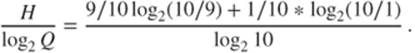
and its average length is ![]() . Therefore, the average length of this code is
. Therefore, the average length of this code is ![]() and, when compared to the code over
and, when compared to the code over ![]() (codewords in
(codewords in ![]() have length 2),
have length 2), ![]() , which is better than the code over the original source.
, which is better than the code over the original source.
One can still improve this encoding scheme considering the source ![]() . It is also possible to refine the encoding with a better model for the source: often the occurrence of some symbol is not independent of the previous symbols issued by the source (e.g., as for a text). In that case, the probabilities of occurrence are conditional and there exist some models (in particular the Markov model) that enable a better encoding. Nevertheless, such processes do not lead to infinite improvements. Entropy remains a threshold for the average length, under which there is no code.
. It is also possible to refine the encoding with a better model for the source: often the occurrence of some symbol is not independent of the previous symbols issued by the source (e.g., as for a text). In that case, the probabilities of occurrence are conditional and there exist some models (in particular the Markov model) that enable a better encoding. Nevertheless, such processes do not lead to infinite improvements. Entropy remains a threshold for the average length, under which there is no code.
Exercise 2.5 One wishes to encode successive throws (one assumes these are infinite) of an unfair die. The symbols of the source are denoted by (1,2,3,4,5,6), and they follow the probability law of occurrence (0.12, 0.15, 0.16, 0.17, 0.18, 0.22).
1. What is the entropy of this source?
2. Propose a ternary code (over some alphabet with three digits) generated by the Huffman algorithm for this source. What is its average length? What minimum average length can we expect for such a ternary code?
3. Same question for a binary code.
Solution on page 296.
Exercise 2.6 (Sequel of the previous exercise)
The Huffman algorithm builds a code in which source words of fixed length are encoded with codewords of varying lengths. The organization of the memory in which the code is stored sometimes imposes a fixed length for codewords. Thus, one encodes sequences of digits of varying length from the source to meet this constraint.
Tunstall codes are optimal codes following this principle. Here is the construction method for the case of a binary alphabet. If the chosen length for codewords is k, one has to find the ![]() sequences of digits from the source one wishes to encode. At the beginning, the set of candidates is the set of words of length 1 (here, {1,2,3,4,5,6}). Let us consider—in this set—the most probable word (here, 6). One builds all possible sequences when adding a digit to this word, and this word is replaced by these sequences in the set of candidates (here, one gets {1,2,3,4,5,61,62,63,64,65,66}). Then, one restarts this operation while having the size of the set strictly lower than
sequences of digits from the source one wishes to encode. At the beginning, the set of candidates is the set of words of length 1 (here, {1,2,3,4,5,6}). Let us consider—in this set—the most probable word (here, 6). One builds all possible sequences when adding a digit to this word, and this word is replaced by these sequences in the set of candidates (here, one gets {1,2,3,4,5,61,62,63,64,65,66}). Then, one restarts this operation while having the size of the set strictly lower than ![]() (one stops before rising above this value).
(one stops before rising above this value).
1. Over some binary alphabet, build the Tunstall code for the die, for codewords of length ![]() .
.
2. 2. What is the codeword associated to the sequence “6664” with the Tunstall? with the Huffman?
3. For each codeword, compute the number of necessary bits of code per character of the source. Deduce the average length per bit of the source of the Tunstall code.
Solution on page 297.
2.2.2 Arithmetic Encoding
Arithmetic encoding is a statistical method that is often better than the Huffman encoding! Yet, we have seen that the Huffman code is optimal, so what kind of optimization is possible? In arithmetic encoding, each character can be encoded on a noninteger number of bits: entire strings of characters of various sizes are encoded on a single integer or a computer real number. For instance, if some character appears with a probability 0.9, the optimal size of the encoding of this character should be
Thus the optimal encoding is around ![]() bits per character, whereas an algorithm such as Huffman's would certainly use an entire bit. Thus, we are going to see how arithmetic encoding enables one to do better.
bits per character, whereas an algorithm such as Huffman's would certainly use an entire bit. Thus, we are going to see how arithmetic encoding enables one to do better.
2.2.2.1 Floating Point Arithmetics
The idea of arithmetic encoding is to encode the characters using intervals. The output of an arithmetic code is a simple real number between 0 and 1 that is built the in following way: to each symbol is associated a subdivision of the interval ![]() whose size is equal to its probability of occurrence. The order of the association does not matter, provided that it is the same for encoding and decoding. For example, a source and the associated intervals are given in the following table.
whose size is equal to its probability of occurrence. The order of the association does not matter, provided that it is the same for encoding and decoding. For example, a source and the associated intervals are given in the following table.
A message will be encoded with a number chosen in the interval whose bounds contain the information of the message. For each character of the message, one refines the interval by allocating the subdivision corresponding to this character. For instance, if the current interval is ![]() and one encodes the character b, then one allocates the subdivision
and one encodes the character b, then one allocates the subdivision ![]() related to
related to ![]() ; hence,
; hence, ![]() .
.
If the message one wishes to encode is “bebecafdead,” then one obtains the real interval ![]() . The steps in the calculation are presented in Table 2.1. Let us choose, for example, “0.15633504500.” The encoding process is very simple, and it can be explained in broad outline in Algorithm 2.2.
. The steps in the calculation are presented in Table 2.1. Let us choose, for example, “0.15633504500.” The encoding process is very simple, and it can be explained in broad outline in Algorithm 2.2.
Table 2.1 Arithmetic Encoding of “bebecafdead”
|
Symbol |
Lower bound |
Upper bound |
|
b |
0.1 |
0.2 |
|
e |
0.15 |
0.19 |
|
b |
0.154 |
0.158 |
|
e |
0.1560 |
0.1576 |
|
c |
0.15632 |
0.15648 |
|
a |
0.156320 |
0.156336 |
|
f |
0.1563344 |
0.1563360 |
|
d |
0.15633488 |
0.15633520 |
|
e |
0.156335040 |
0.156335168 |
|
a |
0.156335040 |
0.1563350528 |
|
d |
0.15633504384 |
0.15633504640 |
For decoding, it is sufficient to locate the interval in which lies “0.15633504500”: namely, ![]() . Thus, the first letter is a “b.”
. Thus, the first letter is a “b.”
Table 2.2 Arithmetic Decoding of “0.15633504500”
|
Real number |
Interval |
Symbol |
Size |
|
0.15633504500 |
[0.1,0.2[ |
b |
0.1 |
|
0.5633504500 |
[0.5,0.9[ |
e |
0.4 |
|
0.158376125 |
[0.1,0.2[ |
b |
0.1 |
|
0.58376125 |
[0.5,0.9[ |
e |
0.4 |
|
0.209403125 |
[0.2,0.3[ |
c |
0.1 |
|
0.09403125 |
[0.0,0.1[ |
a |
0.1 |
|
0.9403125 |
[0.9,1.0[ |
f |
0.1 |
|
0.403125 |
[0.3,0.5[ |
d |
0.2 |
|
0.515625 |
[0.5,0.9[ |
e |
0.4 |
|
0.0390625 |
[0.0,0.1[ |
a |
0.1 |
|
0.390625 |
[0.3,0.5[ |
d |
0.2 |
Then, one has to consider the next interval by subtracting the lowest value and dividing by the size of the interval containing “b,” namely, ![]() . This new number indicates that the next value is a “e.” The sequel of the decoding process is presented in Table 2.2, and the program is described in Algorithm 2.3.
. This new number indicates that the next value is a “e.” The sequel of the decoding process is presented in Table 2.2, and the program is described in Algorithm 2.3.
Remark 2.13
Note that the stopping criterion ![]() of Algorithm 2.3 is valid only if the input number is the lower bound of the interval obtained during encoding. Otherwise, any element of the interval is returned, as in the previous example, another stopping criterion must be provided to the decoding process. This could be, for instance,
of Algorithm 2.3 is valid only if the input number is the lower bound of the interval obtained during encoding. Otherwise, any element of the interval is returned, as in the previous example, another stopping criterion must be provided to the decoding process. This could be, for instance,
· the exact number of symbols to be decoded (this could typically be given as a header in the compressed file).
· another possibility is to use a special character (such as EOF) added to the end of the message to be encoded. This special character could be assigned to the lowest probability.
In summary, encoding progressively reduces the interval proportionately to the probabilities of the characters. Decoding performs the inverse operation, increasing the size of this interval.
2.2.2.2 Integer Arithmetics
The previous encoding depends on the size of the mantissa in the computer representation of real numbers; thus it might not be completely portable. Therefore, it is not used, as it is with floating point arithmetics. Decimal numbers are rather issued one by one in a way that fits the number of bits of the computer word. Integer arithmetics is then more natural than floating point arithmetics: instead of a floating point interval [0,1), an integer interval of the type [00000,99999] is used. Then, encoding is the same. For example, a first occurrence of “b” (using the frequencies in Table 2.1) gives [10000,19999], then “e” would give [15000,18999].
Then one can notice that as soon as the most significant number is identical in the two bounds of the interval, it does not change anymore. Thus it can be printed on the output and subtracted in the integer numbers representing the bounds. This enables one to manipulate only quite small numbers for the bounds. For the message “bebecafdead,” the first occurrence of “b” gives [10000,19999], one prints “1” and subtracts it; hence, the interval becomes [00000,99999]. Then, the “e” gives [50000,89999]; the sequel is given in Table 2.3. The result is 156335043840.
Table 2.3 Integer Arithmetic Encoding of “bebecafdead”
|
Symbol |
Lower bound |
Upper bound |
Output |
|
b |
10000 |
19999 |
|
|
Shift 1 |
00000 |
99999 |
1 |
|
e |
50000 |
89999 |
|
|
b |
54000 |
57999 |
|
|
Shift 5 |
40000 |
79999 |
5 |
|
e |
60000 |
75999 |
|
|
c |
63200 |
64799 |
|
|
Shift 6 |
32000 |
47999 |
6 |
|
a |
32000 |
33599 |
|
|
Shift 3 |
20000 |
35999 |
3 |
|
f |
34400 |
35999 |
|
|
Shift 3 |
44000 |
59999 |
3 |
|
d |
48800 |
51999 |
|
|
e |
50400 |
51679 |
|
|
Shift 5 |
04000 |
16799 |
5 |
|
a |
04000 |
05279 |
|
|
Shift 0 |
40000 |
52799 |
0 |
|
d |
43840 |
46399 |
|
|
43840 |
Decoding almost follows the same procedure by only reading a fixed number of digits at the same time: at each step, one finds the interval (and thus the character) containing the current integer. Then if the most significant digit is identical for both the current integer and the bounds, one shifts the whole set of values as presented in Table 2.4.
Table 2.4 Integer Arithmetic Decoding of “156335043840”
|
Shift |
Integer |
Lower bound |
Upper bound |
Output |
|
15633 |
|
|
b |
|
|
1 |
56335 |
00000 |
99999 |
|
|
56335 |
|
|
e |
|
|
56335 |
|
|
b |
|
|
5 |
63350 |
40000 |
79999 |
|
|
63350 |
|
|
e |
|
|
63350 |
|
|
c |
|
|
6 |
33504 |
32000 |
47999 |
|
|
33504 |
|
|
a |
|
|
3 |
35043 |
20000 |
35999 |
|
|
35043 |
|
|
f |
|
|
3 |
50438 |
44000 |
59999 |
|
|
50438 |
|
|
d |
|
|
50438 |
|
|
e |
|
|
5 |
04384 |
04000 |
16799 |
|
|
04384 |
|
|
a |
|
|
0 |
43840 |
40000 |
52799 |
|
|
43840 |
|
|
d |
2.2.2.3 In Practice
This encoding scheme encounters problems if the two most significant digits do not become equal throughout the encoding. The size of the integers bounding the interval increases, but it can not increase endlessly because of the limitations in any machine. One confronts this issue if he/she gets an interval such as ![]() . After a few additonal iterations, the interval converges toward
. After a few additonal iterations, the interval converges toward ![]() and nothing else is printed!
and nothing else is printed!
To overcome this problem, one has to compare the most significant digits and also the next ones if the latters differ only by 1. Then, if the next ones are 9 and 0, one has to shift them and remember that the shift occurred at the second most significant digit. For example, ![]() is shifted into
is shifted into ![]() ; index 1 meaning that the shift occured at the second digit. Then, when the most significant digits become equal (after k shifts of 0 and 9), one will have to print this number, followed by k 0's or k 9's. In decimal or hexadecimal format, one has to store an additional bit indicating whether the convergence is upwards or downwards; in binary format, this information can be immediately deduced.
; index 1 meaning that the shift occured at the second digit. Then, when the most significant digits become equal (after k shifts of 0 and 9), one will have to print this number, followed by k 0's or k 9's. In decimal or hexadecimal format, one has to store an additional bit indicating whether the convergence is upwards or downwards; in binary format, this information can be immediately deduced.
Exercise 2.7 With the probabilities (“a”: ![]() ; “b”:
; “b”: ![]() ; “c”:
; “c”: ![]() ), the encoding of the string “bbbbba” is given as follows:
), the encoding of the string “bbbbba” is given as follows:
Using the same probabilities, decode the string ![]() . Solution on page 297.
. Solution on page 297.
2.2.3 Adaptive Codes
The encoding scheme represented by the Huffman tree (when considering source extensions) or arithmetic encoding are statistical encodings working on the source model introduced in Chapter 1. Namely, these are based on the knowledge a priori of the frequency of the characters in the file. Moreover, these encoding schemes require a lookup table (or a tree) correlating the source words and the codewords to be able to decompress. This table might become very large when considering source extensions.
Exercise 2.8 Let us consider an alphabet of four characters (“a”,“b”,“c”,“d”) of probability law (1/2,1/6,1/6,1/6).
1. Give the lookup table of the static Huffman algorithm for this source.
2. Assuming that characters a, b, c, and d are written in ASCII (8 bits), what is the minimum memory space required to store this table?
3. What would be the memory space required in order to store the lookup table of the extension of the source on three characters?
4. What is the size of the ASCII file containing the plaintext sequence “aaa aaa aaa bcd bcd bcd”?
5. Compress this sequence with the static Huffman code. Give the overall size of the compressed file. Is it interesting to use an extension of the source?
Solution on page 297.
In practice, there exists dynamic variants (on-the-fly) enabling one to avoid the precomputation of both frequencies and lookup tables. These variants are often used in compression. They use character frequencies, and they calculate them as the symbols occur.
2.2.3.1 Dynamic Huffman's Algorithm—pack
The dynamic Huffman algorithm enables one to compress a stream on-the-fly performing a single reading of the input; contrary to the static Huffman algorithm, this method avoids performing two scans of an input file (one for the computation of the frequencies and the other for the encoding). The frequency table is built as the reading of the file goes on; hence, the Huffman tree is modified each time one reads a character.
The Unix “ pack” command implements this dynamic algorithm.
2.2.3.2 Dynamic Compression
Compression is described in Algorithm 2.4. One assumes that the file to be encoded contains binary symbols, which are read on-the-fly on the form of blocks of k bits (k is often a parameter); therefore, such a block is called a character”. At the initialization phase, one defines a symbolic character (denoted by ![]() in the sequel) initially encoded with a predefined symbol (e.g., the symbolic 257th character in the ASCII code). During the encoding, each time one meets a new unknown character, one encodes it on the output with the code of
in the sequel) initially encoded with a predefined symbol (e.g., the symbolic 257th character in the ASCII code). During the encoding, each time one meets a new unknown character, one encodes it on the output with the code of ![]() followed by the k bits of the new character. The new character is then introduced in the Huffman tree.
followed by the k bits of the new character. The new character is then introduced in the Huffman tree.
In order to build the Huffman tree and update it, one enumerates the number of occurrences of each character as well as the number of characters already read in the file; therefore, one knows, at each reading of a character, the frequency of each character from the beginning of the file to the current character; thus the frequencies are dynamically computed.
After having written a code (either the code of ![]() , or the code of an already known character, or the k uncompressed bits of a new character), one increases by 1 the number of occurrences of the character that has just been written. Taking the frequency modifications into account, one updates the Huffman tree at each step.
, or the code of an already known character, or the k uncompressed bits of a new character), one increases by 1 the number of occurrences of the character that has just been written. Taking the frequency modifications into account, one updates the Huffman tree at each step.
Therefore, the tree exists for compression (and decompression), but there is no need to send it to the decoder.
Possibly there are several choices for the number of occurrences of ![]() : in Algorithm 2.4, it is the number of distinct characters (this enables one to have few bits for
: in Algorithm 2.4, it is the number of distinct characters (this enables one to have few bits for ![]() at the beginning), but it is also possible to provide it, for example, with a constant value close to zero (in that case, the number of bits for
at the beginning), but it is also possible to provide it, for example, with a constant value close to zero (in that case, the number of bits for ![]() evolves according to the depth of the Huffman tree that lets the most frequent characters have the shortest codes).
evolves according to the depth of the Huffman tree that lets the most frequent characters have the shortest codes).
2.2.3.3 Dynamic Decompression
Dynamic decompression is described in Algorithm 2.5. At the initialization, the decoder knows one single code, that of ![]() (e.g., 0). First it reads 0 which we suppose to be the code associated to
(e.g., 0). First it reads 0 which we suppose to be the code associated to ![]() . It deduces that the next k bits contain a new character. It prints thesek bits on its output and updates the Huffman tree, which already contains
. It deduces that the next k bits contain a new character. It prints thesek bits on its output and updates the Huffman tree, which already contains ![]() , with this new character.
, with this new character.
Notice that the coder and the decoder maintain their own Huffman's trees, but they both use the same algorithm in order to update it from the occurrences (frequencies) of the characters that have already been read. Hence, the Huffman trees computed separately by the coder and the decoder are exactly the same.
Then, the decoder reads the next codeword and decodes it using its Huffman's tree. If the codeword represents symbol ![]() , it reads the k bits corresponding to a new character, writes them on its output, and introduces the new character in its Huffman's tree (from now on, the new character is associated with some code). Otherwise, the codeword represents an already known character; using its Huffman's tree, it recovers the k bits of the character associated with the codeword and writes them on its output. Then it increases by 1 the number of occurrences of the character it has just written (and of
, it reads the k bits corresponding to a new character, writes them on its output, and introduces the new character in its Huffman's tree (from now on, the new character is associated with some code). Otherwise, the codeword represents an already known character; using its Huffman's tree, it recovers the k bits of the character associated with the codeword and writes them on its output. Then it increases by 1 the number of occurrences of the character it has just written (and of ![]() in case of a new character) and updates the Huffman tree.
in case of a new character) and updates the Huffman tree.
This dynamic method is a little bit less efficient than the static method for estimating the frequencies. The encoded message is likely to be a little bit longer. However, it avoids the storage of both the tree and the frequency table, which often make the final result shorter. This explains why it is used in practice in common compression utilities.
Exercise 2.9 (Once again, one considers the sequence “aaa aaa aaa bcd bcd bcd”)
1. What would be the dynamic Huffman code of this sequence?
2. What would be the dynamic Huffman code of the extension on three characters of this sequence?
Solution on page 298.
2.2.3.4 Adaptive Arithmetic Encoding
The general idea of the adaptive encoding that has just been developed for the Huffman algorithm is the following:
· At each step, the current code corresponds to the static code one would have obtained using the occurrences already known to compute the frequencies.
· After each step, the encoder updates its occurrence table with the new character it has just received and builds a new static code corresponding to this table. This must always be done in the same way, so that the decoder is able to do the same when its turn comes.
This idea can also be easily implemented dealing with arithmetic encoding: the code is mainly built on the same model as arithmetic encoding, except that the probability distribution is computed on-the-fly by the encoder on the symbols that have already been handled. The decoder is able to perform the same computations, hence, to remain synchronized. An adaptive arithmetic encoder works on floating point arithmetic: at the first iteration, the interval ![]() is divided into segments of same size.
is divided into segments of same size.
Each time a symbol is received, the algorithm computes the new probability distribution and the segment of the symbol is divided into new segments. But the lengths of these new segments now correspond to the updated probabilities of the symbols. The more the symbols are received, the closer the computed probability is to the real probability. As in the case of the dynamic Huffman encoding, there is no overhead because of the preliminary sending of the frequency table and, for variable sources, the encoder is able to dynamically adapt to the variations in the probabilities.
Possibly not only does arithmetic encoding often offer a better compression, but one should also notice that although the static Huffman implementations are faster than the static arithmetic encoding implementations, in general, it is the contrary in the adaptive arithmetic case.
All materials on the site are licensed Creative Commons Attribution-Sharealike 3.0 Unported CC BY-SA 3.0 & GNU Free Documentation License (GFDL)
If you are the copyright holder of any material contained on our site and intend to remove it, please contact our site administrator for approval.
© 2016-2026 All site design rights belong to S.Y.A.