OpenGL SuperBible: Comprehensive Tutorial and Reference, Sixth Edition (2013)

Part I: Foundations

Chapter 3. Following the Pipeline

What You’ll Learn in This Chapter

• What each of the stages in the OpenGL pipeline does

• How to connect your shaders to the fixed-function pipeline stages

• How to create a program that uses every stage of the graphics pipeline simultaneously

In this chapter, we will walk all the way along the OpenGL pipeline from start to finish, providing insight into each of the stages, which include fixed-function blocks and programmable shader blocks. You have already read a whirlwind introduction to the vertex and fragment shader stages. However, the application that you constructed simply drew a single triangle at a fixed position. If we want to render anything interesting with OpenGL, we’re going to have to learn a lot more about the pipeline and all of the things you can do with it. This chapter introduces every part of the pipeline, hooks them up to each other, and provides an example shader for each stage.

Passing Data to the Vertex Shader

The vertex shader is the first programmable stage in the OpenGL pipeline and has the distinction of being the only mandatory stage in the pipeline. However, before the vertex shader runs, a fixed-function stage known as vertex fetching, or sometimes vertex pulling, is run. This automatically provides inputs to the vertex shader.

Vertex Attributes

In GLSL, the mechanism for getting data in and out of shaders is to declare global variables with the in and out storage qualifiers. You were briefly introduced to the out qualifier back in Chapter 2 when Listing 2.4 used it to output a color from the fragment shader. At the start of the OpenGL pipeline, we use the in keyword to bring inputs into the vertex shader. Between stages, in and out can be used to form conduits from shader to shader and pass data between them. We’ll get to that shortly. For now, consider the input to the vertex shader and what happens if you declare a variable with an in storage qualifier. This marks the variable as an input to the vertex shader, which means that it is automatically filled in by the fixed-function vertex fetch stage. The variable becomes known as a vertex attribute.

Vertex attributes are how vertex data is introduced into the OpenGL pipeline. To declare a vertex attribute, declare a variable in the vertex shader using the in storage qualifier. An example of this is shown in Listing 3.1, where we declare the variable offset as an input attribute.

#version 430 core

// "offset" is an input vertex attribute
layout (location = 0) in vec4 offset;

void main(void)
{
const vec4 vertices[3] = vec4[3](vec4( 0.25, -0.25, 0.5, 1.0),
vec4(-0.25, -0.25, 0.5, 1.0),
vec4( 0.25, 0.25, 0.5, 1.0));

// Add "offset" to our hard-coded vertex position
gl_Position = vertices[gl_VertexID] + offset;
}

Listing 3.1: Declaration of a vertex attribute

In Listing 3.1, we have added the variable offset as an input to the vertex shader. As it is an input to the first shader in the pipeline, it will be filled automatically by the vertex fetch stage. We can tell this stage what to fill the variable with by using one of the many variants of the vertex attribute functions, glVertexAttrib*(). The prototype for glVertexAttrib4fv(), which we use in this example, is

void glVertexAttrib4fv(GLuint index,
const GLfloat * v);

Here, the parameter index is used to reference the attribute and v is a pointer to the new data to put into the attribute. You may have noticed the layout (location = 0) code in the declaration of the offset attribute. This is a layout qualifier, and we have used it to set the location of the vertex attribute to zero. This location is the value we’ll pass in index to refer to the attribute.

Each time we call glVertexAttrib*(), it will update the value of the vertex attribute that is passed to the vertex shader. We can use this to animate our one triangle. Listing 3.2 shows an updated version of our rendering function that updates the value of offset in each frame.

// Our rendering function
virtual void render(double currentTime)
{
const GLfloat color[] = { (float)sin(currentTime) * 0.5f + 0.5f,
(float)cos(currentTime) * 0.5f + 0.5f,
0.0f, 1.0f };
glClearBufferfv(GL_COLOR, 0, color);

// Use the program object we created earlier for rendering
glUseProgram(rendering_program);

GLfloat attrib[] = { (float)sin(currentTime) * 0.5f,
(float)cos(currentTime) * 0.6f,
0.0f, 0.0f };

// Update the value of input attribute 0
glVertexAttrib4fv(0, attrib);

// Draw one triangle
glDrawArrays(GL_TRIANGLES, 0, 3);
}

Listing 3.2: Updating a vertex attribute

When we run the program with the rendering function of Listing 3.2, the triangle will move in a smooth oval shape around the window.

Passing Data from Stage to Stage

So far, you have seen how to pass data into a vertex shader by creating a vertex attribute using the in keyword, how to communicate with fixed-function blocks by reading and writing built-in variables such as gl_VertexID and gl_Position, and how to output data from the fragment shader using the out keyword. However, it’s also possible to send your own data from shader stage to shader stage using the same in and out keywords. Just as you used the out keyword in the fragment shader to create the output variable that it writes its color values to, you can create an output variable in the vertex shader by using the out keyword as well. Anything you write to output variables in one shader get sent to similarly named variables declared with the in keyword in the subsequent stage. For example, if your vertex shader declares a variable called vs_color using the outkeyword, it would match up with a variable named vs_color declared with the in keyword in the fragment shader stage (assuming no other stages were active in between).

If we modify our simple vertex shader as shown in Listing 3.3 to include vs_color as an output variable, and correspondingly modify our simple fragment shader to include vs_color as an input variable as shown in Listing 3.4, we can pass a value from the vertex shader to the fragment shader. Then, rather than outputting a hard-coded value, the fragment can simply output the color passed to it from the vertex shader.

#version 430 core

// "offset" and "color" are input vertex attributes
layout (location = 0) in vec4 offset;
layout (location = 1) in vec4 color;

// "vs_color" is an output that will be sent to the next shader stage
out vec4 vs_color;

void main(void)
{
const vec4 vertices[3] = vec4[3](vec4( 0.25, -0.25, 0.5, 1.0),
vec4(-0.25, -0.25, 0.5, 1.0),
vec4( 0.25, 0.25, 0.5, 1.0));

// Add "offset" to our hard-coded vertex position
gl_Position = vertices[gl_VertexID] + offset;

// Output a fixed value for vs_color
vs_color = color;
}

Listing 3.3: Vertex shader with an output

As you can see in Listing 3.3, we declare a second input to our vertex shader, color (this time at location 1), and write its value to the vs_output output. This is picked up by the fragment shader of Listing 3.4 and written to the framebuffer. This allows us to pass a color all the way from a vertex attribute that we can set with glVertexAttrib*() through the vertex shader, into the fragment shader and out to the framebuffer, meaning that we can draw different colored triangles!

#version 430 core

// Input from the vertex shader
in vec4 vs_color;

// Output to the framebuffer
out vec4 color;

void main(void)
{
// Simply assign the color we were given by the vertex shader
// to our output
color = vs_color;
}

Listing 3.4: Fragment shader with an input

Interface Blocks

Declaring interface variables one at a time is possibly the simplest way to communicate data between shader stages. However, in most non-trivial applications, you may wish to communicate a number of different pieces of data between stages, and these may include arrays, structures, and other complex arrangements of variables. To achieve this, we can group together a number of variables into an interface block. The declaration of an interface block looks a lot like a structure declaration, except that it is declared using the in or out keyword depending on whether it is an input to or output from the shader. An example interface block definition is shown in Listing 3.5.

#version 430 core

// "offset" is an input vertex attribute
layout (location = 0) in vec4 offset;
layout (location = 1) in vec4 color;

// Declare VS_OUT as an output interface block
out VS_OUT
{
vec4 color; // Send color to the next stage
} vs_out;

void main(void)
{
const vec4 vertices[3] = vec4[3](vec4( 0.25, -0.25, 0.5, 1.0),
vec4(-0.25, -0.25, 0.5, 1.0),
vec4( 0.25, 0.25, 0.5, 1.0));

// Add "offset" to our hard-coded vertex position
gl_Position = vertices[gl_VertexID] + offset;

// Output a fixed value for vs_color
vs_out.color = color;
}

Listing 3.5: Vertex shader with an output interface block

Note that the interface block in Listing 3.5 has both a block name (VS_OUT, upper case) and an instance name (vs_out, lower case). Interface blocks are matched between stages using the block name (VS_OUT in this case), but are referenced in shaders using the instance name. Thus, modifying our fragment shader to use an interface block gives the code shown in Listing 3.6.

#version 430 core

// Declare VS_OUT as an input interface block
in VS_OUT
{
vec4 color; // Send color to the next stage
} fs_in;

// Output to the framebuffer
out vec4 color;

void main(void)
{
// Simply assign the color we were given by the vertex shader
// to our output
color = fs_in.color;
}

Listing 3.6: Fragment shader with an input interface block

Matching interface blocks by block name but allowing block instances to have different names in each shader stage serves two important purposes: First, it allows the name by which you refer to the block to be different in each stage, avoiding confusing things such as having to use vs_out in a fragment shader, and second, it allows interfaces to go from being single items to arrays when crossing between certain shader stages, such as the vertex and tessellation or geometry shader stages as we will see in a short while. Note that interface blocks are only for moving data from shader stage to shader stage — you can’t use them to group together inputs to the vertex shader or outputs from the fragment shader.

Tessellation

Tessellation is the process of breaking a high-order primitive (which is known as a patch in OpenGL) into many smaller, simpler primitives such as triangles for rendering. OpenGL includes a fixed-function, configurable tessellation engine that is able to break up quadrilaterals, triangles, and lines into a potentially large number of smaller points, lines, or triangles that can be directly consumed by the normal rasterization hardware further down the pipeline. Logically, the tessellation phase sits directly after the vertex shading stage in the OpenGL pipeline and is made up of three parts: the tessellation control shader, the fixed-function tessellation engine, and the tessellation evaluation shader.

Tessellation Control Shaders

The first of the three tessellation phases is the tessellation control shader (sometimes known as simply the control shader, or abbreviated to TCS). This shader takes its input from the vertex shader and is primarily responsible for two things: the first being the determination of the level of tessellation that will be sent to the tessellation engine, and the second being the generation of data that will be sent to the tessellation evaluation shader that is run after tessellation has occurred.

Tessellation in OpenGL works by breaking down high-order surfaces known as patches into points, lines, or triangles. Each patch is formed from a number of control points. The number of control points per patch is configurable and set by calling glPatchParameteri() with pname set toGL_PATCH_VERTICES and value set to the number of control points that will be used to construct each patch. The prototype of glPatchParameteri() is

void glPatchParameteri(GLenum pname,
GLint value);

By default, the number of control points per patch is three, and so if this is what you want (as in our example application), you don’t need to call it at all. When tessellation is active, the vertex shader runs once per control point whilst the tessellation control shader runs in batches on groups of control points where the size of each batch is the same as the number of vertices per patch. That is, vertices are used as control points, and the result of the vertex shader is passed in batches to the tessellation control shader as its input. The number of control points per patch can be changed such that the number of control points that is output by the tessellation control shader can be different from the number of control points that it consumes. The number of control points produced by the control shader is set using an output layout qualifier in the control shader’s source code. Such a layout qualifier looks like:

layout (vertices = N) out;

Here, N is the number of control points per patch. The control shader is responsible for calculating the values of the output control points and for setting the tessellation factors for the resulting patch that will be sent to the fixed-function tessellation engine. The output tessellation factors are written to the gl_TessLevelInner and gl_TessLevelOuter built-in output variables, whereas any other data that is passed down the pipeline is written to user-defined output variables (those declared using the out keyword, or the special built-in gl_out array) as normal.

Listing 3.7 shows a simple tessellation control shader. It sets the number of output control points to three (the same as the default number of input control points) using the layout (vertices = 3) out; layout qualifier, copies its input to its output (using the built-in variables gl_in and gl_out), and sets the inner and outer tessellation level to 5. The built-in input variable gl_InvocationID is used to index into the gl_in and gl_out arrays. This variable contains the zero-based index of the control point within the patch being processed by the current invocation of the tessellation control shader.

#version 430 core

layout (vertices = 3) out;

void main(void)
{
if (gl_InvocationID == 0)
{
gl_TessLevelInner[0] = 5.0;
gl_TessLevelOuter[0] = 5.0;
gl_TessLevelOuter[1] = 5.0;
gl_TessLevelOuter[2] = 5.0;
}
gl_out[gl_InvocationID].gl_Position = gl_in[gl_InvocationID].gl_Position;
}

Listing 3.7: Our first tessellation control shader

The Tessellation Engine

The tessellation engine is a fixed-function part of the OpenGL pipeline that takes high-order surfaces represented as patches and breaks them down into simpler primitives such as points, lines, or triangles. Before the tessellation engine receives a patch, the tessellation control shader processes the incoming control points and sets tessellation factors that are used to break down the patch. After the tessellation engine produces the output primitives, the vertices representing them are picked up by the tessellation evaluation shader. The tessellation engine is responsible for producing the parameters that are fed to the invocations of the tessellation evaluation shader, which it then uses to transform the resulting primitives and get them ready for rasterization.

Tessellation Evaluation Shaders

Once the fixed-function tessellation engine has run, it produces a number of output vertices representing the primitives it has generated. These are passed to the tessellation evaluation shader. The tessellation evaluation shader (evaluation shader, or TES for short) runs an invocation for eachvertex produced by the tessellator. When the tessellation levels are high, this means that the tessellation evaluation shader could run an extremely large number of times, and so you should be careful with complex evaluation shaders and high tessellation levels.

Listing 3.8 shows a tessellation evaluation shader that accepts input vertices produced by the tessellator as a result of running the control shader shown in Listing 3.7. At the start of the shader is a layout qualifier that sets the tessellation mode. In this case, we selected that the mode should be triangles. Other qualifiers, equal_spacing and cw, select that new vertices should be generated equally spaced along the tessellated polygon edges and that a clockwise vertex winding order should be used for the generated triangles. We will cover the other possible choices in the section “Tessellation” in Chapter 8.

In the remainder of the shader, you will see that it assigns a value to gl_Position just like a vertex shader does. It calculates this using the contents of two more built-in variables. The first is gl_TessCoord, which is the barycentric coordinate of the vertex generated by the tessellator. The second is the gl_Position member of the gl_in[] array of structures. This matches the gl_out structure written to in the tessellation control shader earlier in Listing 3.7. This shader essentially implements pass-through tessellation. That is, the tessellated output patch is the exact same shape as the original, incoming triangular patch.

#version 430 core

layout (triangles, equal_spacing, cw) in;

void main(void)
{
gl_Position = (gl_TessCoord.x * gl_in[0].gl_Position +
gl_TessCoord.y * gl_in[1].gl_Position +
gl_TessCoord.z * gl_in[2].gl_Position);
}

Listing 3.8: Our first tessellation evaluation shader

In order to see the results of the tessellator, we need to tell OpenGL to draw only the outlines of the resulting triangles. To do this, we call glPolygonMode(), whose prototype is

void glPolygonMode(GLenum face,
GLenum mode);

The face parameter specifies what type of polygons we want to affect and as we want to affect everything, we set it to GL_FRONT_AND_BACK. The other modes will be explained shortly. mode says how we want our polygons to be rendered. As we want to render in wireframe mode (i.e., lines), we set this to GL_LINE. The result of rendering our one triangle example with tessellation enabled and the two shaders of Listing 3.7 and Listing 3.8 is shown in Figure 3.1.

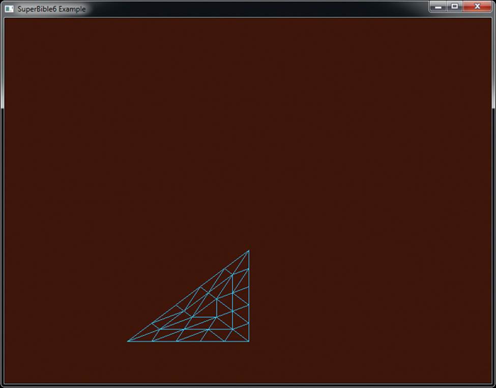
Figure 3.1: Our first tessellated triangle

Geometry Shaders

The geometry shader is logically the last shader stage in the front end, sitting after vertex and tessellation stages and before the rasterizer. The geometry shader runs once per primitive and has access to all of the input vertex data for all of the vertices that make up the primitive being processed. The geometry shader is also unique amongst the shader stages in that it is able to increase or reduce the amount of data flowing in through the pipeline in a programmatic way. Tessellation shaders can also increase or decrease the amount of work in the pipeline, but only implicitly by setting the tessellation level for the patch. Geometry shaders, on the other hand, include two functions — EmitVertex() and EndPrimitive() — that explicitly produce vertices that are sent to primitive assembly and rasterization.

Another unique feature of geometry shaders is that they can change the primitive mode mid-pipeline. For example, they can take triangles as input and produce a bunch of points or lines as output, or even create triangles from independent points. An example geometry shader is shown inListing 3.9.

#version 430 core

layout (triangles) in;
layout (points, max_vertices = 3) out;

void main(void)
{
int i;

for (i = 0; i < gl_in.length(); i++)
{
gl_Position = gl_in[i].gl_Position;
EmitVertex();
}
}

Listing 3.9: Our first geometry shader

The shader shown in Listing 3.9 acts as another simple pass-through shader that converts triangles into points so that we can see their vertices. The first layout qualifier indicates that the geometry shader is expecting to see triangles as its input. The second layout qualifier tells OpenGL that the geometry shader will produce points and that the maximum number of points that each shader will produce will be three. In the main function, we have a loop that runs through all of the members of the gl_in array, which is determined by calling its .length() function.

We actually know that the length of the array will be three because we are processing triangles and every triangle has three vertices. The outputs of the geometry shader are again similar to those of a vertex shader. In particular, we write to gl_Position to set the position of the resulting vertex. Next, we call EmitVertex(), which produces a vertex at the output of the geometry shader. Geometry shaders automatically call EndPrimitive() for you at the end of your shader, and so calling it explicitly is not necessary in this example. As a result of running this shader, three vertices will be produced and they will be rendered as points.

By inserting this geometry shader into our simple one tessellated triangle example, we obtain the output shown in Figure 3.2. To create this image, we set the point size to 5.0 by calling glPointSize(). This makes the points large and highly visible.

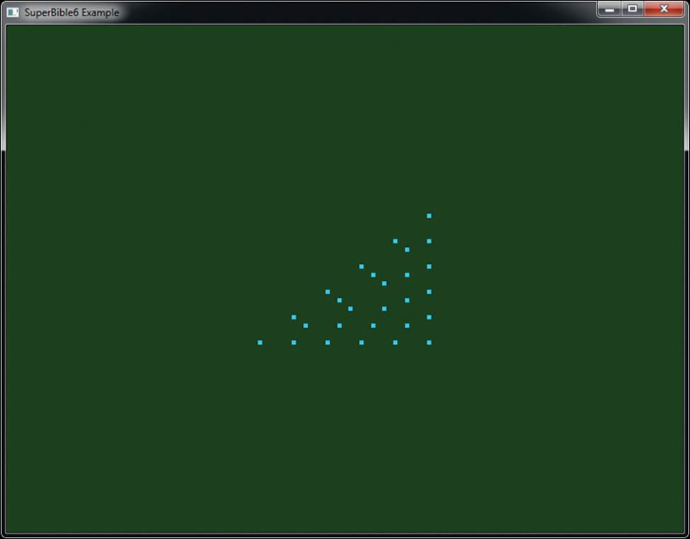
Figure 3.2: Tessellated triangle after adding a geometry shader

Primitive Assembly, Clipping, and Rasterization

After the front end of the pipeline has run (which includes vertex shading, tessellation, and geometry shading) comes a fixed-function part of the pipeline that performs a series of tasks that take the vertex representation of our scene and convert it into a series of pixels that in turn need to be colored and written to the screen. The first step in this process is primitive assembly, which is the grouping of vertices into lines and triangles. Primitive assembly still occurs for points, but it is trivial in that case. Once primitives have been constructed from their individual vertices, they areclipped against the displayable region, which usually means the window or screen, but can be a smaller area known as the viewport. Finally, the parts of the primitive that are determined to be potentially visible are sent to a fixed-function subsystem called the rasterizer. This block determines which pixels are covered by the primitive (point, line, or triangle) and sends the list of pixels on to the next stage, which is fragment shading.

Clipping

As vertices exit the vertex shader, their position is said to be in clip space. This is one of the many coordinate systems that can be used to represent positions. You may have noticed that the gl_Position variable that we have written to in our vertex, tessellation, and geometry shaders has a vec4type and that the positions that we have produced by writing to it are all four-component vectors. This is what is known as a homogeneous coordinate. The homogeneous coordinate system is used in projective geometry as much of the math ends up simpler in homogeneous coordinate space than it does in a regular Cartesian space. Homogeneous coordinates have one more component than their equivalent Cartesian coordinate, which is why our three-dimensional position vector is represented as a four-component variable.

Although the output of the front end is a four-component homogeneous coordinate, clipping occurs in Cartesian space, and so to convert from homogeneous coordinates to Cartesian coordinates, OpenGL performs a perspective division, which is the process of dividing all four components of the position by the last component, w. This has the effect of projecting the vertex from the homogeneous space to the Cartesian space, leaving w as 1.0. In all of the examples so far, we have set the w component of gl_Position as 1.0, and so this division has no effect. When we explore projective geometry in a short while, we will discuss the effect of setting w to values other than one.

After the projective division, the resulting position is now in normalized device space. In OpenGL, the visible region of normalized device space is the volume that extends from −1.0 to 1.0 in the x and y dimensions and from 0.0 to 1.0 in the z dimension. Any geometry that is contained in this region may become visible to the user, and anything outside of it should be discarded. The six sides of this volume are formed by planes in three-dimensional space. As a plane divides a coordinate space in two, the volumes on each side of the plane are called half-spaces.

Before passing primitives on to the next stage, OpenGL performs clipping by determining which side of each of these planes the vertices of each primitive lie on. Each plane effectively has an “outside” and an “inside.” If a primitive’s vertices all lie on the “outside” of any one plane, then the whole thing is thrown away. If all of primitive’s vertices are on the “inside” of all the planes (and therefore inside the view volume), then it is passed through unaltered. Primitives that are partially visible (which means that they cross one of the planes) must be handled specially. More details about how this works is given in the section “Clipping” in Chapter 7.

Viewport Transformation

After clipping, all of the vertices of your geometry have coordinates that lie between −1.0 and 1.0 in the x and y dimensions. Along with a z coordinate that lies between 0.0 and 1.0, these are known as normalized device coordinates. However, the window that you’re drawing to has coordinates that start from (0, 0) at the bottom left and range to (w – 1, h – 1), where w and h are the width and height of the window in pixels, respectively. In order to place your geometry into the window, OpenGL applies the viewport transform, which applies a scale and offset to the vertices’ normalized device coordinates to move them into window coordinates. The scale and bias to apply are determined by the viewport bounds, which you can set by calling glViewport() and glDepthRange().

This transform takes the form

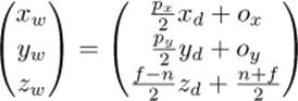
Here, x_w, y_w, and z_w are the resulting coordinates of the vertex in window space, and x_d, y_d, and z_d are the incoming coordinates of the vertex in normalized device space. p_x and p_y are the width and height of the viewport, in pixels, and n and f are the near and far plane distances in the zcoordinate, respectively. Finally, o_x, o_y, and o_z are the origins of the viewport.

Culling

Before a triangle is processed further, it may be optionally passed through a stage called culling, which determines whether the triangle faces towards or away from the viewer and can decide whether to actually go ahead and draw it based on the result of this computation. If the triangle faces towards the viewer, then it is considered to be front-facing; otherwise, it is said to be back-facing. It is very common to discard triangles that are back-facing because when an object is closed, any back-facing triangle will be hidden by another front-facing triangle.

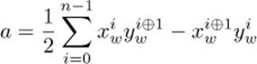
To determine whether a triangle is front- or back-facing, OpenGL will determine its signed area in window space. One way to determine the area of a triangle is to take the cross product of two of its edges. The equation for this is

Here, and are the coordinates of the i^th vertex of the triangle in window space, and i ⊕ 1 is (i + 1) mod 3. If the area is positive, then the triangle is considered to be front-facing, and if it is negative, then it is considered to be back-facing. The sense of this computation can be reversed by calling glFrontFace() with either dir set to either GL_CW or GL_CCW (where CW and CCW stand for clockwise and counter clockwise, respectively). This is known as the winding order of the triangle, and the clockwise or counterclockwise terms refer to the order in which the vertices appear in window space. By default, this state is set to GL_CCW, indicating that triangles whose vertices are in counterclockwise order are considered to be front-facing and those whose vertices are in clockwise order are considered to be back-facing. If the state is GL_CW, then a is simply negated before being used in the culling process. Figure 3.3 shows this pictorially for the purpose of illustration.

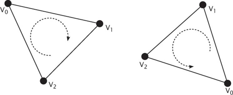
Figure 3.3: Clockwise (left) and counterclockwise (right) winding order

Once the direction that the triangle is facing has been determined, OpenGL is capable of discarding either front-facing, back-facing, or even both types of triangles. By default, OpenGL will render all triangles, regardless of which way they face. To turn on culling, call glEnable() with cap set to GL_CULL_FACE. When you enable culling, OpenGL will cull back-facing triangles by default. To change which types of triangles are culled, call glCullFace() with face set to GL_FRONT, GL_BACK, or GL_FRONT_AND_BACK.

As points and lines don’t have any geometric¹ area, this facing calculation doesn’t apply to them and they can’t be culled at this stage.

1. Obviously, once they are rendered to the screen, points and lines have area; otherwise, we wouldn’t be able to see them. However, this area is artificial and can’t be calculated directly from their vertices.

Rasterization

Rasterization is the process of determining which fragments might be covered by a primitive such as a line or a triangle. There are a myriad of algorithms for doing this, but most OpenGL systems will settle on a half-space-based method for triangles as it lends itself well to parallel implementation. Essentially, OpenGL will determine a bounding box for the triangle in window coordinates and test every fragment inside it to determine whether it is inside or outside the triangle. To do this, it treats each of the triangle’s three edges as a half-space that divides the window in two.

Fragments that lie on the interior of all three edges are considered to be inside the triangle, and fragments that lie on the exterior of any of the three edges are considered to be outside the triangle. Because the algorithm to determine which side of a line a point lies on is relatively simple and is independent of anything besides the position of the line’s endpoints and of the point being tested, many tests can be performed concurrently, providing the opportunity for massive parallelism.

Fragment Shaders

The fragment² shader is the last programmable stage in OpenGL’s graphics pipeline. This stage is responsible for determining the color of each fragment before it is sent to the framebuffer for possible composition into the window. After the rasterizer processes a primitive, it produces a list of fragments that need to be colored and passes it to the fragment shader. Here, an explosion in the amount of work in the pipeline occurs as each triangle could produce hundreds, thousands, or even millions of fragments.

2. The term fragment is used to describe an element that may ultimately contribute to the final color of a pixel. The pixel may not end up being the color produced by any particular invocation of the fragment shader due to a number of other effects such as depth or stencil tests, blending, or multi-sampling, all of which will be covered later in the book.

Listing 2.4 back in Chapter 2 contains the source code of our first fragment shader. It’s an extremely simple shader that declares a single output and then assigns a fixed value to it. In a real-world application, the fragment shader would normally be substantially more complex and be responsible for performing calculations related to lighting, applying materials, and even determining the depth of the fragment. Available as input to the fragment shader are several built-in variables such as gl_FragCoord, which contains the position of the fragment within the window. It is possible to use these variables to produce a unique color for each fragment.

Listing 3.10 provides a shader that derives its output color from gl_FragCoord, and Figure 3.4, shows the output of running our original single-triangle program with this shader installed.

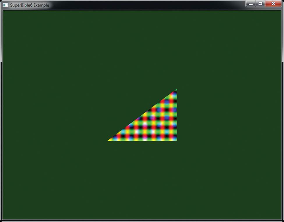
Figure 3.4: Result of Listing 3.10

#version 430 core

out vec4 color;

void main(void)
{
color = vec4(sin(gl_FragCoord.x * 0.25) * 0.5 + 0.5,
cos(gl_FragCoord.y * 0.25) * 0.5 + 0.5,
sin(gl_FragCoord.x * 0.15) * cos(gl_FragCoord.y * 0.15),
1.0);
}

Listing 3.10: Deriving a fragment’s color from its position

As you can see, the color of each pixel in Figure 3.4 is now a function of its position, and a simple screen-aligned pattern has been produced. It is the shader of Listing 3.10 that created the checkered patterns in the output.

The gl_FragCoord variable is one of the built-in variables available to the fragment shader. However, just as with other shader stages, we can define our own inputs to the fragment shader, which will be filled in based on the outputs of whichever stage is last before rasterization. For example, if we have a simple program with only a vertex shader and fragment shader in it, we can pass data from the fragment shader to the vertex shader.

The inputs to the fragment shader are somewhat unlike inputs to other shader stages in that OpenGL interpolates their values across the primitive that’s being rendered. To demonstrate, we take the vertex shader of Listing 3.3 and modify it to assign a different, fixed color for each vertex, as shown in Listing 3.11.

#version 430 core

// "vs_color" is an output that will be sent to the next shader stage
out vec4 vs_color;

void main(void)
{
const vec4 vertices[3] = vec4[3](vec4( 0.25, -0.25, 0.5, 1.0),
vec4(-0.25, -0.25, 0.5, 1.0),
vec4( 0.25, 0.25, 0.5, 1.0));
const vec4 colors[] = vec4[3](vec4( 1.0, 0.0, 0.0, 1.0),
vec4( 0.0, 1.0, 0.0, 1.0),
vec4( 0.0, 0.0, 1.0, 1.0));
// Add "offset" to our hard-coded vertex position
gl_Position = vertices[gl_VertexID] + offset;

// Output a fixed value for vs_color
vs_color = color[gl_VertexID];
}

Listing 3.11: Vertex shader with an output

As you can see, in Listing 3.11, we added a second constant array that contains colors and index into it using gl_VertexID, writing its content to the vs_color output. Now, we modify our simple fragment shader to include the corresponding input and write its value to the output, as shown inListing 3.12.

#version 430 core

// "vs_color" is the color produced by the vertex shader
in vec4 vs_color;

out vec4 color;

void main(void)
{
color = vs_color;
}

Listing 3.12: Deriving a fragment’s color from its position

The result of using this new pair of shaders is shown in Figure 3.5. As you can see, the color changes smoothly across the triangle.

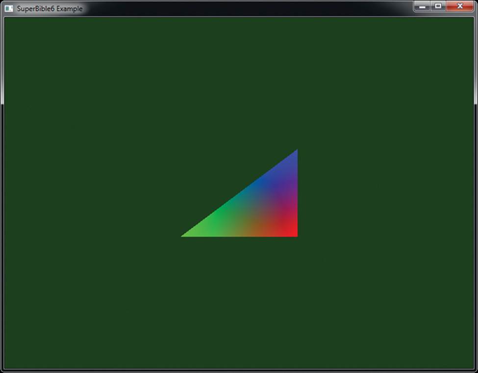
Figure 3.5: Result of Listing 3.12

Framebuffer Operations

The framebuffer represents the last stage of the OpenGL graphics pipeline. It can represent the visible content of the screen and a number of additional regions of memory that are used to store per-pixel values other than color. On most platforms, this means the window you see on your desktop (or possibly the whole screen if your application covers it) and it is owned by the operating system (or windowing system to be more precise). The framebuffer provided by the windowing system is known as the default framebuffer, but it is possible to provide your own if you wish to do things like render into off-screen areas. The state held by the framebuffer includes states such as where the data produced by your fragment shader should be written, what the format of that data should be, and so on. This state is stored in an object, called a framebuffer object. Also considered part of the framebuffer, but not stored per framebuffer object, is the pixel operation state.

Pixel Operations

After the fragment shader has produced an output, several things may happen to the fragment before it is written to the window, such as whether it even belongs in the window. Each of these things may be turned on or off by your application. The first thing that could happen is the scissor test, which tests your fragment against a rectangle that you can define. If it’s inside the rectangle, then it’ll get processed further, and if it’s outside, it’ll get thrown away.

Next comes the stencil test. This compares a reference value provided by your application with the contents of the stencil buffer, which stores a single³ value per-pixel. The content of the stencil buffer has no particular semantic meaning and can be used for any purpose.

3. It’s actually possible for a framebuffer to store multiple depth, stencil, or color values per-pixel when a technique called multi-sampling is employed. We’ll dig into this later in the book.

After the stencil test has been performed, a second test called the depth test is performed. The depth test is an operation that compares the fragment’s z coordinate against the contents of the depth buffer. The depth buffer is a region of memory that, like the stencil buffer, is another part of the framebuffer with enough space for a single value for each pixel, and it contains the depth (which is related to distance from the viewer) of each pixel.

Normally, the values in the depth buffer range from zero to one, with zero being the closest possible point in the depth buffer and one being the furthest possible point in the depth buffer. To determine whether a fragment is closer than other fragments that have already been rendered in the same place, OpenGL can compare the z component of the fragment’s window-space coordinate against the value already in the depth buffer, and if it is less than what’s already there, then the fragment is visible. The sense of this test can also be changed. For example, you can ask OpenGL to let fragments through that have a z coordinate that is greater than, equal to, or not equal to the content of the depth buffer. The result of the depth test also affects what OpenGL does to the stencil buffer.

Next, the fragment’s color is sent either to the blending or logical operation stage, depending on whether the framebuffer is considered to store floating-point, normalized, or integer values. If the content of the framebuffer is either floating-point or normalized integer values, then blending is applied. Blending is a highly configurable stage in OpenGL and will be covered in detail in its own section. In short, OpenGL is capable of using a wide range of functions that take components of the output of your fragment shader and of the current content of the framebuffer and calculate new values that are written back to the framebuffer. If the framebuffer contains unnormalized integer values, then logical operations such as logical AND, OR, and XOR can be applied to the output of your shader and the value currently in the framebuffer to produce a new value that will be written back into the framebuffer.

Compute Shaders

The first sections of this chapter describe the graphics pipeline in OpenGL. However, OpenGL also includes the compute shader stage, which can almost be thought of as a separate pipeline that runs independently of the other graphics-oriented stages.

Compute shaders are a way of getting at the computational power possessed by the graphics processor in the system. Unlike the graphics-centric vertex, tessellation, geometry, and fragment shaders, compute shaders could be considered as a special, single-stage pipeline all on their own. Each invocation of the compute shader operates on a single unit of work known as a work item, several of which are formed together into small groups called local workgroups. Collections of these workgroups can be sent into OpenGL’s compute pipeline to be processed. The compute shader doesn’t have any fixed inputs or outputs besides a handful of built-in variables to tell the shader which item it’s working on. All processing performed by a compute shader is explicitly written to memory by the shader itself rather than being consumed by a subsequent pipeline stage. A very basic compute shader is shown in Listing 3.13.

#version 430 core

layout (local_size_x = 32, local_size_y = 32) in;

void main(void)
{
// Do nothing
}

Listing 3.13: Simple do-nothing compute shader

Compute shaders are otherwise just like any other shader stage in OpenGL. To compile one, you create a shader object with the type GL_COMPUTE_SHADER, attach your GLSL source code to it with glShaderSource(), compile it with glCompileShader(), and then link it into a program withglAttachShader() and glLinkProgram(). The result is a program object with a compiled compute shader in it that can be launched to do work for you.

The shader in Listing 3.13 tells OpenGL that the size of the local workgroup is going to be 32 by 32 work items, but then proceeds to do nothing. In order to make a compute shader that actually does something useful, you’re going to need to know a bit more about OpenGL, and so we’ll revisit this later in the book.

Summary

In this chapter, you have taken a whirlwind trip down OpenGL’s graphics pipeline. You have been (very) briefly introduced to each major stage and have created a program that uses each of them, if only to do nothing impressive. We’ve glossed over or even neglected to mention several useful features of OpenGL with the intention of getting you from zero to rendering in as few pages as possible. Over the next few chapters, you’ll learn more fundamentals of computer graphics and of OpenGL, and then we’ll take a second trip down the pipeline, dig deeper into the topics from this chapter, and get into some of the things we skipped in this preview of what OpenGL can do.