THE RUBY WAY, Third Edition (2015)
Chapter 5. Performing Numerical Calculations
On two occasions I have been asked [by members of Parliament], “Pray, Mr. Babbage, if you put into the machine wrong figures, will the right answers come out?” I am not able rightly to apprehend the kind of confusion of ideas that could provoke such a question.
—Charles Babbage
Numeric data is the original data type, the native language of the computer. We would be hard-pressed to find areas of our experience where numbers are not applicable. It doesn’t matter whether you’re an accountant or an aeronautical engineer; you can’t survive without numbers. We present in this chapter a few ways to process, manipulate, convert, and analyze numeric data.
Like all modern languages, Ruby works well with both integers and floating point numbers. It has the full range of standard mathematical operators and functions that you would expect, but it also has a few pleasant surprises such as the Bignum, BigDecimal, and Rational classes.
Besides covering all of the numeric features in the core and standard libraries, a little domain-specific material has been added (in such areas as trigonometry, calculus, and statistics). These examples serve not only as informative examples in math, but as examples of Ruby code that illustrates principles from the rest of this book.
5.1 Representing Numbers in Ruby
If you know any other language, the representation of numbers in Ruby is mostly intuitive. A Fixnum may be signed or unsigned:
237 # unsigned (positive) number
+237 # same as above
-237 # negative number
When numbers have many digits, we can insert underscores at will (between any two digits). This is purely cosmetic and does not affect the value of the constant. Typically, we would insert them at the same places where accountants might insert commas:
1048576 # a simple number
1_048_576 # the same value
It’s also possible to represent integers in the most common alternative bases (bases 2, 8, and 16). These are “tagged” with the prefixes 0b, 0, and 0x, respectively:
0b10010110 # binary
0b1211 # error!
01234 # octal (base 8)
01823 # error!
0xdeadbeef # hexadecimal (base 16)
0xDEADBEEF # same
0xdeadpork # error!
Floating point numbers have to have a decimal point and may optionally have a signed exponent:
3.14 # pi to two digits
-0.628 # -2*pi over 10, to two digits
6.02e23 # Avogadro's number
6.626068e-34 # Planck's constant
Certain constants in the Float class help define limits for floating point numbers. These are machine dependent. Some of the more important follow:
Float::MIN # 2.2250738585072e-308 (on this machine)
Float::MAX # 1.79769313486232e+308
Float::EPSILON # 2.22044604925031e-16
5.2 Basic Operations on Numbers
The normal operations of addition, subtraction, multiplication, and division are implemented in Ruby, much as in the typical programming language with the operators +, -, *, and /. Most of the operators are actually methods (and therefore can be overridden).
Exponentiation (raising to a power) is done with the ** operator, as in older languages such as BASIC and FORTRAN. The operator obeys the “normal” mathematical laws of exponentiation:
a = 64**2 # 4096
b = 64**0.5 # 8.0
c = 64**0 # 1
d = 64**-1 # 0.015625
Division of one integer by another results in a truncated integer. This is a feature, not a bug. If you need a floating point number, make sure that at least one operand is a floating point:
3 / 3 # 3
5 / 3 # 1
3 / 4 # 0
3.0 / 4 # 0.75
3 / 4.0 # 0.75
3.0 / 4.0 # 0.75
If you are using variables and are in doubt about the division, Float or to_f will ensure that an operand is a floating point number:
z = x.to_f / y
z = Float(x) / y
See also Section 5.17, “Performing Bit-Level Operations on Numbers,” later in this chapter.
5.3 Rounding Floating Point Values
Kirk: What would you say the odds are on our getting out of here?
Spock: It is difficult to be precise, Captain. I should say approximately 7824.7 to one.
—Star Trek, “Errand of Mercy”
If you want to round a floating point value to an integer, the method round will do the trick:
pi = 3.14159
new_pi = pi.round # 3
temp = -47.6
temp2 = temp.round # -48
Sometimes we want to round not to an integer but to a specific number of decimal places. In this case, we would pass the desired number of digits after the decimal to round:
pi = 3.1415926535
pi6 = pi.round(6) # 3.141593
pi5 = pi.round(5) # 3.14159
pi4 = pi.round(4) # 3.1416
Occasionally we follow a different rule in rounding to integers. The tradition of rounding n+0.5 upward results in slight inaccuracies at times; after all, n+0.5 is no closer to n+1 than it is to n. So there is an alternative tradition that rounds to the nearest even number in the case of 0.5as a fractional part. If we wanted to do this, we might extend the Float class with a method of our own called round_down, as shown here:
class Float
def round_down
whole = self.floor
fraction = self - whole
if fraction == 0.5
if (whole % 2) == 0
whole
else
whole+1
end
else
self.round
end
end
end
a = (33.4).round_down # 33
b = (33.5).round_down # 34
c = (33.6).round_down # 34
d = (34.4).round_down # 34
e = (34.5).round_down # 34
f = (34.6).round_down # 35
Obviously, round_down differs from round only when the fractional part is exactly 0.5; note that 0.5 can be represented perfectly in binary, by the way. What is less obvious is that this method works fine for negative numbers also. (Try it.) Also note that the parentheses used here are not actually necessary but are used for readability.
As an aside, it should be obvious that adding a method to a system class is something that should be done with caution and awareness. Though there are times and places where this practice is appropriate, it is easy to overdo. These examples are shown primarily for ease of illustration, not as a suggestion that this sort of code should be written frequently.
Now, what if we wanted to round to a number of decimal places, but we wanted to use the “even rounding” method? In this case, we could add a parameter to round_down:
class Float
def roundf_down(places = 0)
shift = 10 ** places
num = (self * shift).round_down / shift.to_f
num.round(places)
end
end
a = 6.125
b = 6.135
x = a.roundf_down(2) # 6.12
y = b.roundf_down(2) # 6.14
z = b.roundf_down # 6
The roundf_down method has certain limitations. Large floating point numbers might overflow when multiplied by a large power of ten. For these occurrences, error-checking should be added.
5.4 Comparing Floating Point Numbers
It is a sad fact of life that computers do not represent floating point values exactly. The following code fragment, in a perfect world, would print “yes”; on every architecture we have tried, it will print “no” instead:
x = 1000001.0/0.003
y = 0.003*x
if y == 1000001.0
puts "yes"
else
puts "no"
end
The reason, of course, is that a floating point number is stored in some finite number of bits, and no finite number of bits is adequate to store a repeating decimal with an infinite number of digits.
Because of this inherent inaccuracy in floating point comparisons, we may find ourselves in situations (like the one we just saw) where the values we are comparing are the same for all practical purposes, but the hardware stubbornly thinks they are different.
The following code is a simple way to ensure that floating point comparisons are done “with a fudge factor”—that is, the comparisons will be done within any tolerance specified by the programmer:
class Float
EPSILON = 1e-6 # 0.000001
def ==(x)
(self-x).abs < EPSILON
end
end
x = 1000001.0/0.003
y = 0.003*x
if y == 1.0 # Using the new ==
puts "yes" # Now we output "yes"
else
puts "no"
end
We may find that we want different tolerances for different situations. For this case, we define a new method, nearly_equal?, as a member of Float. (This name avoids confusion with the standard methods equal? and eql?; the latter in particular should not be overridden.)
class Float
EPSILON = 1e-6
def nearly_equal?(x, tolerance=EPSILON)
(self-x).abs < tolerance
end
end
flag1 = (3.1416).nearly_equal? Math::PI # false
flag2 = (3.1416).nearly_equal?(Math::PI, 0.001) # true
We could also use a different operator entirely to represent approximate equality; the =~ operator might be a good choice.
Bear in mind that this sort of thing is not a real solution. As successive computations are performed, error is compounded. If you must use floating point math, be prepared for the inaccuracies. If the inaccuracies are not acceptable, use BigDecimal or some other solution. (See Section 5.8, “Using BigDecimal,” and Section 5.9, “Working with Rational Values,” later in the chapter.)
5.5 Formatting Numbers for Output
To output numbers in a specific format, you can use the printf method in the Kernel module. It is virtually identical to its C counterpart. For more information, see the documentation for the printf method:
x = 345.6789
i = 123
printf("x = %6.2f\n", x) # x = 345.68
printf("x = %9.2e\n", x) # x = 3.457e+02
printf("i = %5d\n", i) # i = 123
printf("i = %05d\n", i) # i = 00123
printf("i = %-5d\n", i) # i = 123
To store a result in a string rather than printing it immediately, sprintf can be used in much the same way. The following method returns a string:
str = sprintf("%5.1f",x) # "345.7"
Finally, the String class has the % method, which performs this same task. The % method has a format string as a receiver; it takes a single argument (or an array of values) and returns a string:
# Usage is 'format % value'
str = "%5.1f" % x # "345.7"
str = "%6.2f, %05d" % [x,i] # "345.68, 00123"
5.6 Formatting Numbers with Commas
There may be better ways to format numbers with commas, but this one works. We reverse the string to make it easier to do global substitution and then reverse it again at the end:
def commas(x)
str = x.to_s.reverse
str.gsub!(/([0-9]{3})/,"\\1,")
str.gsub(/,$/,"").reverse
end
puts commas(123) # "123"
puts commas(1234) # "1,234"
puts commas(12345) # "12,435"
puts commas(123456) # "123,456"
puts commas(1234567) # "1,234,567"
5.7 Working with Very Large Integers
The control of large numbers is possible, and like unto that of small numbers, if we subdivide them.
—Sun Tze
In the event it becomes necessary, Ruby programmers can work with integers of arbitrary size. The transition from a Fixnum to a Bignum is handled automatically and transparently. In this following piece of code, notice how a result that is large enough is promoted from Fixnum toBignum:
num1 = 1000000 # One million (10**6)
num2 = num1*num1 # One trillion (10**12)
puts num1 # 1000000
puts num1.class # Fixnum
puts num2 # 1000000000000
puts num2.class # Bignum
The size of a Fixnum varies from one architecture to another. Calculations with Bignums are limited only by memory and processor speed. They take more memory and are obviously somewhat slower, but number-crunching with very large integers (hundreds of digits) is still reasonably practical.
5.8 Using BigDecimal
The Bigdecimal standard library enables us to work with large numbers of significant digits in fractional numbers. In effect, it stores numbers as arrays of digits rather than converting to a binary floating point representation. This allows arbitrary precision, though of course at the cost of speed.
To motivate ourselves, look at the following simple piece of code using floating point numbers:
if (3.2 - 2.0) == 1.2
puts "equal"
else
puts "not equal" # prints "not equal"!
end
This is the sort of situation that BigDecimal helps with. However, note that with infinitely repeating decimals, we still will have problems. For yet another approach, see Section 5.9, “Working with Rational Values.”
A BigDecimal is initialized with a string. (A Float would not suffice because the error would creep in before we could construct the BigDecimal object.) The method BigDecimal is equivalent to BigDecimal.new; this is another special case where a method name starts with a capital letter. The usual mathematical operations such as + and * are supported. Note that the to_s method can take a parameter to specify its format. For more details, see the BigDecimal documentation.
require 'bigdecimal'
x = BigDecimal("3.2")
y = BigDecimal("2.0")
z = BigDecimal("1.2")
if (x - y) == z
puts "equal" # prints "equal"!
else
puts "not equal"
end
a = x*y*z
a.to_s # "0.768E1" (default: engineering notation)
a.to_s("F") # "7.68" (ordinary floating point)
We can specify the number of significant digits if we want. The precs method retrieves this information as an array of two numbers: the number of bytes used and the maximum number of significant digits.
x = BigDecimal("1.234",10)
y = BigDecimal("1.234",15)
x.precs # [8, 16]
y.precs # [8, 20]
The bytes currently used may be less than the maximum. The maximum may also be greater than what you requested (because BigDecimal tries to optimize its internal storage).
The common operations (addition, subtraction, multiplication, and division) have counterparts that take a number of digits as an extra parameter. If the resulting significant digits are more than that parameter specifies, the result will be rounded to that number of digits.
a = BigDecimal("1.23456")
b = BigDecimal("2.45678")
# In these comments, "BigDecimal:objectid" is omitted
c = a+b # <'0.369134E1',12(20)>
c2 = a.add(b,4) # <'0.3691E1',8(20)>
d = a-b # <'-0.122222E1',12(20)>
d2 = a.sub(b,4) # <'-0.1222E1',8(20)>
e = a*b # <'0.3033042316 8E1',16(36)>
e2 = a.mult(b,4) # <'0.3033E1',8(36)>
f = a/b # <'0.5025114173 8372992290 7221E0',24(32)>
f2 = a.div(b,4) # <'0.5025E0',4(16)>
The BigDecimal class defines many other functions, such as floor, abs, and others. There are operators such as % and **, as you would expect, along with relational operators such as <. The == operator is not intelligent enough to round off its operands; that is still the programmer’s responsibility.
The BigMath module defines constants E and PI to arbitrary precision. (They are really methods, not constants.) It also defines functions such as sin, cos, exp, and others, all taking a digits parameter.
The following sublibraries are all made to work with BigDecimal:
• bigdecimal/math—The BigMath module.
• bigdecimal/jacobian—Methods for finding a Jacobian matrix.
• bigdecimal/ludcmp—The LUSolve module, for LU decomposition.
• bigdecimal/newton—Provides nlsolve and norm.
These sublibraries are not documented in this chapter. For more information, consult the ruby-doc.org site or any detailed reference.
5.9 Working with Rational Values
The Rational class enables us (in many cases) to work with fractional values with “infinite” precision. It helps us only when the values involved are true rational numbers (the quotient of two integers). It won’t help with irrational numbers such as pi, e, or the square root of 2.
To create a rational number, we use the special method Rational (which is one of our rare capitalized method names, usually used for data conversion or initialization):
r = Rational(1,2) # 1/2 or 0.5
s = Rational(1,3) # 1/3 or 0.3333...
t = Rational(1,7) # 1/7 or 0.14...
u = Rational(6,2) # "same as" 3.0
z = Rational(1,0) # error!
An operation on two rationals will typically be another rational:
r+t # Rational(9, 14)
r-t # Rational(5, 14)
r*s # Rational(1, 6)
r/s # Rational(3, 2)
Let’s look once again at our floating point inaccuracy example (see Section 5.4, “Comparing Floating Point Numbers”). In the following example, we do the same thing with rationals rather than reals, and we get the “mathematically expected” results instead:
x = Rational(1000001,1)/Rational(3,1000)
y = Rational(3,1000)*x
if y == 1000001.0
puts "yes" # Now we get "yes"!
else
puts "no"
end
Some operations, of course, don’t always give us rationals back:
x = Rational(9,16) # Rational(9, 16)
Math.sqrt(x) # 0.75
x**0.5 # 0.75
x**Rational(1,2) # 0.75
However, the mathn library changes some of this behavior. See Section 5.12, “Using mathn,” later in this chapter.
5.10 Matrix Manipulation
If you want to deal with numerical matrices, the standard library matrix is for you. This actually defines two separate classes: Matrix and Vector.
You should also be aware of the excellent NArray library by Masahiro Tanaka (available as a gem from rubygems.org). This is not a standard library but is well known and very useful. If you have speed requirements, if you have specific data representation needs, or if you need capabilities such as Fast Fourier Transform, you should definitely look into this package. For most general purposes, however, the standard matrix library should suffice, and that is what we cover here.
To create a matrix, we naturally use a class-level method. There are multiple ways to do this. One way is simply to call Matrix.[] and list the rows as arrays. In the following example, we do this in multiple lines, though of course that isn’t necessary:
m = Matrix[[1,2,3],
[4,5,6],
[7,8,9]]
A similar method is to call rows, passing in an array of arrays (so that the “extra” brackets are necessary). The optional copy parameter, which defaults to true, determines whether the individual arrays are copied or simply stored. Therefore, let this parameter be true to protect the original arrays, or false if you want to save a little memory, and you are not concerned about this issue.
row1 = [2,3]
row2 = [4,5]
m1 = Matrix.rows([row1,row2]) # copy=true
m2 = Matrix.rows([row1,row2],false) # don't copy
row1[1] = 99 # Now change row1
p m1 # Matrix[[2, 3], [4, 5]]
p m2 # Matrix[[2, 99], [4, 5]]
Matrices can similarly be specified in column order with the columns method. It does not accept the copy parameter because the arrays are split up anyway to be stored internally in row-major order:
m1 = Matrix.rows([[1,2],[3,4]])
m2 = Matrix.columns([[1,3],[2,4]]) # m1 == m2
Matrices are assumed to be rectangular. If you assign a matrix with rows or columns that are shorter or longer than the others, you will immediately get an error informing you that your matrix input was not rectangular.
Certain special matrices, especially square ones, are easily constructed. The “identity” matrix can be constructed with the identity method (or its aliases I and unit):
im1 = Matrix.identity(3) # Matrix[[1,0,0],[0,1,0],[0,0,1]]
im2 = Matrix.I(3) # same
im3 = Matrix.unit(3) # same
A more general form is scalar, which assigns some value other than 1 to the diagonal:
sm = Matrix.scalar(3,8) # Matrix[[8,0,0],[0,8,0],[0,0,8]]
Still more general is diagonal, which assigns an arbitrary sequence of values to the diagonal. (Obviously, it does not need the dimension parameter.)
dm = Matrix.diagonal(2,3,7) # Matrix[[2,0,0],[0,3,0],[0,0,7]]
The zero method creates a special matrix of the specified dimension, full of zero values:
zm = Matrix.zero(3) # Matrix[[0,0,0],[0,0,0],[0,0,0]]
Obviously, the identity, scalar, diagonal, and zero methods all construct square matrices.
To create a 1×N or an N×1 matrix, you can use the row_vector or column_vector shortcut methods, respectively:
a = Matrix.row_vector(2,4,6,8) # Matrix[[2,4,6,8]]
b = Matrix.column_vector(6,7,8,9) # Matrix[[6],[7],[8],[9]]
Individual matrix elements can naturally be accessed with the bracket notation (with both indices specified in a single pair of brackets). Note that there is no []= method. This is for much the same reason that Fixnum lacks that method: Matrices are immutable objects (evidently a design decision by the library author).
m = Matrix[[1,2,3],[4,5,6]]
puts m[1,2] # 6
Be aware that indexing is from zero, as with Ruby arrays; this may contradict your mathematical expectation, but there is no option for one-based rows and columns unless you implement it yourself.
# Naive approach... don't do this!
class Matrix
alias bracket []
def [](i,j)
bracket(i-1,j-1)
end
end
m = Matrix[[1,2,3],[4,5,6],[7,8,9]]
p m[2,2] # 5
The preceding code does seem to work. Many or most matrix operations still behave as expected with the alternate indexing. Why might it fail? Because we don’t know all the internal implementation details of the Matrix class. If it always uses its own [] method to access the matrix values, it should always be consistent. But if it ever accesses some internal array directly or uses some kind of shortcut, it might fail. Therefore, if you use this kind of trick at all, it should be with caution and testing.
In reality, you would have to change the row and vector methods as well. These methods use indices that number from zero without going through the [] method. I haven’t checked to see what else might be required.
Sometimes we need to discover the dimensions or shape of a matrix. There are various methods for this purpose, such as row_size and column_size, which return the number of rows and columns in the matrix, respectively.
To retrieve a section or piece of a matrix, several methods are available. The row_vectors method returns an array of Vector objects representing the rows of the matrix. (See the following discussion of the Vector class.) The column_vectors method works similarly. Finally, the minor method returns a smaller matrix from the larger one; its parameters are either four numbers (lower and upper bounds for the rows and columns) or two ranges.
m = Matrix[[1,2,3,4],[5,6,7,8],[6,7,8,9]]
rows = m.row_vectors # three Vector objects
cols = m.column_vectors # four Vector objects
m2 = m.minor(1,2,1,2) # Matrix[[6,7,],[7,8]]
m3 = m.minor(0..1,1..3) # Matrix[[[2,3,4],[6,7,8]]
The usual matrix operations can be applied: addition, subtraction, multiplication, and division. Some of these make certain assumptions about the dimensions of the matrices and may raise exceptions if the operands are incompatible (for example, trying to multiply a 3×3 matrix with a 4×4 matrix).
Ordinary transformations, such as inverse, transpose, and determinant, are supported. For matrices of integers, the determinant will usually be better behaved if the mathn library is used (see the Section 5.12, “Using mathn”).
A Vector is in effect a special one-dimensional matrix. It can be created with the [] or elements method; the first takes an expanded array, and the latter takes an unexpanded array and an optional copy parameter (which defaults to true).
arr = [2,3,4,5]
v1 = Vector[*arr] # Vector[2,3,4,5]
v2 = Vector.elements(arr) # Vector[2,3,4,5]
v3 = Vector.elements(arr,false) # Vector[2,3,4,5]
arr[2] = 7 # v3 is now Vector[2,3,7,5]
The covector method converts a vector of length N to an N×1 (effectively transposed) matrix.
v = Vector[2,3,4]
m = v.covector # Matrix[[2,3,4]]
Addition and subtraction of similar vectors are supported. A vector may be multiplied by a matrix or by a scalar. All these operations are subject to normal mathematical rules.
v1 = Vector[2,3,4]
v2 = Vector[4,5,6]
v3 = v1 + v2 # Vector[6,8,10]
v4 = v1*v2.covector # Matrix[[8,10,12],[12,15,18],[16,20,24]]
v5 = v1*5 # Vector[10,15,20]
There is an inner_product method:
v1 = Vector[2,3,4]
v2 = Vector[4,5,6]
x = v1.inner_product(v2) # 47
For additional information on the Matrix and Vector classes, see the class documentation online or via the ri command.
5.11 Working with Complex Numbers
The standard library complex enables us to handle imaginary and complex numbers in Ruby. Much of it is self-explanatory.
Complex values can be created with this slightly unusual notation:
z = Complex(3,5) # 3+5i
What is unusual about this is that we have a method name that is the same as the class name. In this case, the presence of the parentheses indicates a method call rather than a reference to a constant. In general, method names do not look like constants, and I don’t recommend the practice of capitalizing method names except in special cases like this. (Note that there are also methods called Integer and Float; in general, the capitalized method names are for data conversion or something similar.)
The im method converts a number to its imaginary counterpart (effectively multiplying it by i). Therefore, we can represent imaginary and complex numbers with a more convenient notation:
a = 3.im # 3i
b = 5 - 2.im # 5-2i
If we’re more concerned with polar coordinates, we can also call the polar class method:
z = Complex.polar(5,Math::PI/2.0) # radius, angle
The Complex class also gives us the constant I, which of course represents i, the square root of negative one:
z1 = Complex(3,5)
z2 = 3 + 5*Complex::I # z2 == z1
If you choose to require the complex library, certain common math functions have their behavior changed. Trig functions such as sin, sinh, tan, and tanh (along with others such as exp and log) accept complex arguments in addition to their normal behavior. In some cases, such as sqrt, they are “smart” enough to return complex results also.
x = Math.sqrt(Complex(3,5)) # roughly: Complex(2.1013, 1.1897)
y = Math.sqrt(-1) # Complex(0,1)
For more information, refer the Complex class documentation.
5.12 Using mathn
For math-intensive programs, you will want to know about the mathn library created by Keiju Ishitsuka. It provides a few convenience methods and classes, and replaces many methods in Ruby’s numeric classes so that they “play well” together.
The easiest way to “use” this library is simply to require it and forget it. Because it requires the complex, rational, and matrix libraries (in that order), there is no need to do separate requires of those if you are using them. In general, the mathn library tries to produce “sensible” results from computations—for example, the square root of a Rational will be returned when possible as another Rational rather than a Float. Table 5.1 shows some typical effects of loading this library.
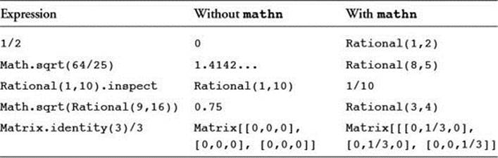
Table 5.1 Computation with and without the mathn Library
The mathn library adds the ** and power2 methods to Rational. It changes the behavior of Math.sqrt and adds the rational-aware function Math.rsqrt.
See also Section 5.13, “Finding Prime Factorization, GCD, and LCM,” and Section 5.14, “Working with Prime Numbers.”
5.13 Finding Prime Factorization, GCD, and LCM
The mathn library also defines some new methods on the Integer class. One is gcd2, which finds the greatest common divisor of the receiver and the other specified number:
n = 36.gcd2(120) # 12
k = 237.gcd2(79) # 79
The prime_division method performs a prime factorization of its receiver. The result returned is an array of arrays where each smaller array consists of a prime number and its exponent:
factors = 126.prime_division # [[2,1], [3,2], [7,1]]
# i.e. 2**1 * 3**2 * 7**1
There is also the class method Integer.from_prime_division, which reverses that factorization. It is a class method because it is like a “constructor” for an integer.
factors = [[2,1],[3,1],[7,1]]
num = Integer.from_prime_division(factors) # 42
The following code is an example of using prime factorization to find the least common multiple (LCM) of a pair of numbers:
require 'mathn'
class Integer
def lcm(other)
pf1 = self.prime_division.flatten
pf2 = other.prime_division.flatten
h1 = Hash[*pf1]
h2 = Hash[*pf2]
hash = h2.merge(h1) {|key,old,new| [old,new].max }
Integer.from_prime_division(hash.to_a)
end
end
p 15.lcm(150) # 150
p 2.lcm(3) # 6
p 4.lcm(12) # 12
p 200.lcm(30) # 600
5.14 Working with Prime Numbers
The mathn library defines a class for generating prime numbers. The iterator each generates these in succession in an infinite loop. The succ method naturally generates the next prime number.
For example, here are two ways to list the first 100 primes:
require 'mathn'
list = []
gen = Prime.new
gen.each do |prime|
list << prime
break if list.size == 100
end
# or alternatively:
list = []
gen = Prime.new
100.times { list << gen.succ }
The following code tests the primality of a number. With large enough numbers, this may take a moment to complete:
require 'mathn'
class Integer
def prime?
max = Math.sqrt(self).ceil
max -= 1 if max % 2 == 0
pgen = Prime.new
pgen.each do |factor|
return false if self % factor == 0
return true if factor > max
end
end
end
31.prime? # true
237.prime? # false
1500450271.prime? # true
5.15 Implicit and Explicit Numeric Conversion
The new Rubyist is often confused that there are methods named to_i and to_int (and by analogy, to_f and to_flt, as well as others). In general, explicit conversion is done using the “short name” and implicit conversion using the “long name.”
What does this mean? First, most classes define explicit convertors but not implicit.
Second, your own classes will tend to define implicit convertors, but you will not usually call them manually (unless you are writing “client” code or library-oriented code that tries to play well with the outside world).
The following code is a contrived example. The class MyClass as defined in this example returns constants from to_i and to_int. This is nonsensical behavior, but it illustrates a point:
class MyClass
def to_i
3
end
def to_int
5
end
end
If we want to convert a MyClass object explicitly to an integer, we can call to_i:
m = MyClass.new
x = m.to_i # 3
But the to_int method gets called implicitly (“behind our backs”) when we pass in a MyClass object to something that expects an integer. For example, suppose that we want to create an array with an initial number of values; Array.new can take an integer, but what happens if we give it a MyClass object instead?
m = MyClass.new
a = Array.new(m) # [nil,nil,nil,nil,nil]
As we see, the new method was smart enough to call to_int and thus create an array with five entries.
For more explanation in a different context (strings), see Section 2.16, “Implicit and Explicit Conversion.” See also the following section, 5.16, “Coercing Numeric Values.”
5.16 Coercing Numeric Values
Coercion can be thought of as another form of implicit conversion. When a method (+ for example) is passed an argument it doesn’t understand, it tries to coerce the receiver and the argument to compatible types and then do the addition based on those types. The pattern for using coerce in a class you write is straightforward:
class MyNumberSystem
def +(other)
if other.kind_of?(MyNumberSystem)
result = some_calculation_between_self_and_other
MyNumberSystem.new(result)
else
n1, n2 = other.coerce(self)
n1 + n2
end
end
end
The value returned by coerce is a two-element array containing its argument and its receiver converted to compatible types.
In this example, we’re relying on the type of our argument to perform some kind of coercion for us. If we want to be good citizens, we also need to implement coercion in our class, allowing other types of numbers to work with us. To do this, we need to know the specific types that we can work with directly and convert to those types when appropriate. When we can’t do that, we fall back on asking our parent class:
def coerce(other)
if other.kind_of?(Float)
return other, self.to_f
elsif other.kind_of?(Integer)
return other, self.to_i
else
super
end
end
Of course, for this to work, our object must implement to_i and to_f.
You can use coerce as part of the solution for implementing a Perl-like autoconversion of strings to numbers:
class String
def coerce(n)
if self['.']
[n, Float(self)]
else
[n, Integer(self)]
end
end
end
x = 1 + "23" # 24
y = 23 * "1.23" # 28.29
This can cause many unexpected results, so we recommend against ever doing this. But we do recommend that you automatically coerce other number types whenever you are creating some kind of numeric class.
5.17 Performing Bit-Level Operations on Numbers
Occasionally we may need to operate on a Fixnum as a binary entity. This is less common in application-level programming, but the need still arises.
Ruby has a relatively full set of capabilities in this area. For convenience, numeric constants may be expressed in binary, octal, or hexadecimal. The usual operators AND, OR, XOR, and NOT are expressed by the Ruby operators &, |, ^, and ~, respectively.
x = 0377 # Octal (decimal 255)
y = 0b00100110 # Binary (decimal 38)
z = 0xBEEF # Hex (decimal 48879)
a = x | z # 48895 (bitwise OR)
b = x & z # 239 (bitwise AND)
c = x ^ z # 48656 (bitwise XOR)
d = ~ y # -39 (negation or 1's complement)
The instance method size can be used to determine the word size of the specific architecture on which the program is running:
bytes = 1.size # Returns 4 for one particular machine
There are left-shift and right-shift operators (<< and >>, respectively). These are logical shift operations; they do not disturb the sign bit (though >> does propagate it).
x = 8
y = -8
a = x >> 2 # 2
b = y >> 2 # -2
c = x << 2 # 32
d = y << 2 # -32
Of course, anything shifted far enough to result in a zero value will lose the sign bit because -0 is merely 0.
Brackets can be used to treat numbers as arrays of bits. The 0th bit is the least significant bit, regardless of the bit order (endianness) of the architecture.
x = 5 # Same as 0b0101
a = x[0] # 1
b = x[1] # 0
c = x[2] # 1
d = x[3] # 0
# Etc. # 0
It is not possible to assign bits using this notation (because a Fixnum is stored as an immediate value rather than an object reference). However, you can always fake it by left-shifting a 1 to the specified bit position and then doing an OR or AND operation.
# We can't do x[3] = 1
# but we can do:
x |= (1<<3)
# We can't do x[4] = 0
# but we can do:
x &= ~(1<<4)
5.18 Performing Base Conversions
Obviously all integers are representable in any base, because they are all stored internally in binary. Further, we know that Ruby can deal with integer constants in any of the four commonly used bases. This means that if we are concerned about base conversions, we must be concerned with strings in some fashion.
If you are concerned with converting a string to an integer, that is covered in Section 2.24, “Converting Strings to Numbers (Decimal and Otherwise).”
If you are concerned with converting numbers to strings, the simplest way is to use the to_s method with the optional base parameter. This naturally defaults to 10, but it does handle bases up to 36 (using all letters of the alphabet).
237.to_s(2) # "11101101"
237.to_s(5) # "1422"
237.to_s(8) # "355"
237.to_s # "237"
237.to_s(16) # "ed"
237.to_s(30) # "7r"
Another way is to use the % method of the String class:
hex = "%x" % 1234 # "4d2"
oct = "%o" % 1234 # "2322"
bin = "%b" % 1234 # "10011010010"
The sprintf method also works:
str = sprintf(str,"Nietzsche is %x\n",57005)
# str is now: "Nietzsche is dead\n"
Obviously, printf will also suffice if you want to print out the value as you convert it.
5.19 Finding Cube Roots, Fourth Roots, and So On
Ruby has a built-in square root function (Math.sqrt) because that function is so commonly used. But what if you need higher-level roots? If you remember your math, this is easy.
One way is to use logarithms. Recall that e to the x is the inverse of the natural log of x, and that when we multiply numbers, that is equivalent to adding their logarithms:
x = 531441
cuberoot = Math.exp(Math.log(x)/3.0) # 81.0
fourthroot = Math.exp(Math.log(x)/4.0) # 27.0
However, it is just as easy and perhaps clearer simply to use fractions with an exponentiation operator (which can take any integer or floating point value):
include Math
y = 4096
cuberoot = y**(1.0/3.0) # 16.0
fourthroot = y**(1.0/4.0) # 8.0
fourthroot = sqrt(sqrt(y)) # 8.0 (same thing)
twelfthroot = y**(1.0/12.0) # 2.0
Note that in all these examples, we have used floating point numbers when dividing (to avoid truncation to an integer).
5.20 Determining the Architecture’s Byte Order
It is an interesting fact of the computing world that we cannot all agree on the order in which binary data ought to be stored. Is the most significant bit stored at the higher-numbered address or the lower? When we shove a message over a wire, do we send the most significant bit first, or the least significant?
Believe it or not, it’s not entirely arbitrary. There are good arguments on both sides (which we will not delve into here).
For more than 30 years, the terms little-endian and big-endian have been applied to the two extreme opposites. These apparently were first used by Danny Cohen; refer to his classic article “On Holy Wars and a Plea for Peace” (IEEE Computer, October 1981). The actual terms are derived from the novel Gulliver’s Travels by Jonathan Swift.
Most of the time, we don’t care what byte order our architecture uses. But what if we do need to know?
The following method determines this for us. It returns a string that is LITTLE, BIG, or OTHER. It depends on the fact that the l directive packs in native mode, and the N directive unpacks in network order (or big-endian):
def endianness
num=0x12345678
little = "78563412"
big = "12345678"
native = [num].pack('l')
netunpack = native.unpack('N')[0]
str = "%8x" % netunpack
case str
when little
"LITTLE"
when big
"BIG"
else
"OTHER"
end
end
puts endianness # In this case, prints "LITTLE"
This technique might come in handy if, for example, you are working with binary data (such as scanned image data) imported from another architecture.
5.21 Numerical Computation of a Definite Integral
I’m very good at integral and differential calculus....
—W. S. Gilbert, The Pirates of Penzance, Act 1
If you want to estimate the value of a definite integral, there is a time-tested technique for doing so. This is what the calculus student will remember as a Riemann sum.
The integrate method shown here takes beginning and ending values for the dependent variable as well as an increment. The fourth parameter (which is not really a parameter) is a block. This block should evaluate a function based on the value of the dependent variable passed into that block. (Here we are using “variable” in the mathematical sense, not in the computing sense.) It is not necessary to define a function to call in this block, but we do so here for clarity:
def integrate(x0, x1, dx=(x1-x0)/1000.0)
x = x0
sum = 0
loop do
y = yield(x)
sum += dx * y
x += dx
break if x > x1
end
sum
end
def f(x)
x**2
end
z = integrate(0.0,5.0) {|x| f(x) }
puts z # 41.72918749999876
Note that in the preceding example, we are relying on the fact that a block returns a value that yield can retrieve. We also make certain assumptions here. First, we assume that x0 is less than x1 (otherwise, an infinite loop results); the reader can easily improve the code in details such as this one. Second, we assume that the function can be evaluated at arbitrary points in the specified domain. If at any time we try to evaluate the function at such a point, chaos will ensue. (Such functions are generally not integrable anyway, at least over that set of x values. Consider the function f(x)=x/(x-3) when x is 3.)
Drawing on our faded memories of calculus, we might compute the result here to be 41.666 or thereabout (5 cubed divided by 3). Why is the answer not as exact as we might like? It is because of the size of the “slice” in the Riemann sum; a smaller value for dx will result in greater accuracy (at the expense of an increase in runtime).
Finally, I will point out that a function like this is more useful when we have a variety of functions of arbitrary complexity, not just a simple function such as f(x) = x**2.
5.22 Trigonometry in Degrees, Radians, and Grads
When it comes to measuring arc, the mathematical or “natural” unit is the radian, defined in such a way that an angle of one radian corresponds to an arc length equal to the radius of the circle. A little thought will show that there are 2π radians in a circle.
The degree of arc, which we use in everyday life, is a holdover from ancient Babylonian base-60 units; this system divides the circle into 360 degrees. The less-familiar grad is a pseudo-metric unit defined in such a way that there are 100 grads in a right angle (or 400 in a circle).
Programming languages often default to the radian when calculating trigonometric functions, and Ruby is no exception. But we show here how to do these calculations in degrees or grads, in the event that any of our readers are engineers or ancient Babylonians.
Because the number of units in a circle is a simple constant, it follows that there are simple conversion factors between all these units. We define these here and simply use the constant names in subsequent code. As a matter of convenience, we’ll stick them in the Math module:
module Math
RAD2DEG = 360.0/(2.0*PI) # Radians to degrees
RAD2GRAD = 400.0/(2.0*PI) # Radians to grads
end
Now we can define new trig functions if we want. Because we are converting to radians in each case, we will divide by the conversion factor we calculated previously. We could place these in the Math module if we wanted, though we don’t show it here:
def sin_d(theta)
Math.sin (theta/Math::RAD2DEG)
end
def sin_g(theta)
Math.sin (theta/Math::RAD2GRAD)
end
Of course, the corresponding cos and tan functions may be similarly defined.
The atan2 function is a little different. It takes two arguments (the opposite and adjacent legs of a right triangle) and returns an angle. Therefore, we convert the result, not the argument, handling it this way:
def atan2_d(y,x)
Math.atan2(y,x)/Math::RAD2DEG
end
def atan2_g(y,x)
Math.atan2(y,x)/Math::RAD2GRAD
end
5.23 Finding Logarithms with Arbitrary Bases
When working with logarithms, we frequently use the natural logarithms (or base e, sometimes written ln); we may also use the common or base 10 logarithms. These are defined in Ruby as Math.log and Math.log10, respectively.
In computer science, specifically in such areas as coding and information theory, a base 2 log is not unusual. For example, this will tell the minimum number of bits needed to store a number. We define this function here as log2:
def log2(x)
Math.log(x)/Math.log(2)
end
The inverse is obviously 2**x, just as the inverse of log x is Math::E**x or Math.exp(x).
Furthermore, this same technique can be extended to any base. In the unlikely event that you ever need a base 7 logarithm, this will do the trick:
def log7(x)
Math.log(x)/Math.log(7)
end
In practice, the denominator should be calculated once and kept around as a constant.
5.24 Finding the Mean, Median, and Mode of a Data Set
Given an array, x, let’s find the mean of all the values in that array. Actually, there are three common kinds of mean. The ordinary or arithmetic mean is what we call the average in everyday life. The harmonic mean is the number of terms divided by the sum of all their reciprocals. And finally, the geometric mean is the nth root of the product of the n values. We show each of these in the following example:
def mean(x)
sum = 0
x.each {|v| sum += v}
sum/x.size
end
def hmean(x)
sum = 0
x.each {|v| sum += (1.0/v)}
x.size/sum
end
def gmean(x)
prod = 1.0
x.each {|v| prod *= v}
prod**(1.0/x.size)
end
data = [1.1, 2.3, 3.3, 1.2, 4.5, 2.1, 6.6]
am = mean(data) # 3.014285714285714
hm = hmean(data) # 2.1019979464765117
gm = gmean(data) # 2.5084114744285384
The median value of a data set is the value that occurs approximately in the middle of the (sorted) set. (The following code fragment computes a median.) For this value, half the numbers in the set should be less, and half should be greater. Obviously, this statistic will be more appropriate and meaningful for some data sets than others. See the following code:
def median(x)
sorted = x.sort
mid = x.size/2
sorted[mid]
end
data = [7,7,7,4,4,5,4,5,7,2,2,3,3,7,3,4]
puts median(data) # 4
The mode of a data set is the value that occurs most frequently. If there is only one such value, the set is unimodal; otherwise, it is multimodal. A multimodal data set is a more complex case that we do not consider here. The interested reader can extend and improve the code we show here:
def mode(x)
f = {} # frequency table
fmax = 0 # maximum frequency
m = nil # mode
x.each do |v|
f[v] ||= 0
f[v] += 1
fmax,m = f[v], v if f[v] > fmax
end
return m
end
data = [7,7,7,4,4,5,4,5,7,2,2,3,3,7,3,4]
puts mode(data) # 7
5.25 Variance and Standard Deviation
The variance of a set of data is a measure of how “spread out” the values are. (Here we do not distinguish between biased and unbiased estimates.) The standard deviation, usually represented by a sigma (σ), is simply the square root of the variance:
data = [2, 3, 2, 2, 3, 4, 5, 5, 4, 3, 4, 1, 2]
def variance(x)
m = mean(x)
sum = 0.0
x.each {|v| sum += (v-m)**2 }
sum/x.size
end
def sigma(x)
Math.sqrt(variance(x))
end
puts variance(data) # 1.4615384615384615
puts sigma(data) # 1.2089410496539776
Note that the variance function in the preceding code uses the mean function defined earlier.
5.26 Finding a Correlation Coefficient
The correlation coefficient is one of the simplest and most universally useful statistical measures. It is a measure of the “linearity” of a set of x-y pairs, ranging from -1.0 (complete negative correlation) to +1.0 (complete positive correlation).
We compute this using the mean and sigma (standard deviation) functions defined previously in Section 5.25, “Variance and Standard Deviation.” For a detailed explanation of this tool, consult a statistics reference such as The Elements of Statistical Learning, available online.
The following version assumes two arrays of numbers (of the same size):
def correlate(x,y)
sum = 0.0
x.each_index do |i|
sum += x[i]*y[i]
end
xymean = sum/x.size.to_f
xmean = mean(x)
ymean = mean(y)
sx = sigma(x)
sy = sigma(y)
(xymean-(xmean*ymean))/(sx*sy)
end
a = [3, 6, 9, 12, 15, 18, 21]
b = [1.1, 2.1, 3.4, 4.8, 5.6]
c = [1.9, 1.0, 3.9, 3.1, 6.9]
c1 = correlate(a,a) # 1.0
c2 = correlate(a,a.reverse) # -1.0
c3 = correlate(b,c) # 0.8221970227633335
The following version is similar, but it operates on a single array, each element of which is an array containing an x-y pair:
def correlate2(v)
sum = 0.0
v.each do |a|
sum += a[0]*a[1]
end
xymean = sum/v.size.to_f
x = v.collect {|a| a[0]}
y = v.collect {|a| a[1]}
xmean = mean(x)
ymean = mean(y)
sx = sigma(x)
sy = sigma(y)
(xymean-(xmean*ymean))/(sx*sy)
end
d = [[1,6.1], [2.1,3.1], [3.9,5.0], [4.8,6.2]]
c4 = correlate2(d) # 0.22778224915306602
Finally, the following version assumes that the x-y pairs are stored in a hash. It simply builds on the previous example:
def correlate_h(h)
correlate2(h.to_a)
end
e = { 1 => 6.1, 2.1 => 3.1, 3.9 => 5.0, 4.8 => 6.2}
c5 = correlate_h(e) # 0.22778224915306602
5.27 Generating Random Numbers
If a pseudorandom number is good enough for you, you’re in luck. This is what most language implementations supply you with, and Ruby is no exception.
The Kernel method rand returns a pseudorandom floating point number, x, such that x>=0.0 and x<1.0. Here is an example (note that yours will vary):
a = rand # 0.6279091137
If it is called with the integer parameter max, it returns an integer in the range 0...max (noninclusive of the upper bound). Here is an example (note that yours will vary):
n = rand(10) # 7
If we want to seed the random number generator, we can do so with the Kernel method srand, which takes a single numeric parameter. If we pass no value to it, it will construct its own using (among other things) the time of day. If we pass a number to it, it will use that number as the seed. This can be useful in testing, when we want a repeatable sequence of pseudorandom numbers from one script invocation to the next:
srand(5)
i, j, k = rand(100), rand(100), rand(100)
# 26, 45, 56
srand(5)
l, m, n = rand(100), rand(100), rand(100)
# 26, 45, 56
5.28 Caching Functions with Memoization
Suppose you have a computationally expensive mathematical function that will be called repeatedly in the course of execution. If speed is critical and you can afford to sacrifice a little memory, it may be effective to store the function results in a table and look them up. This makes the implicit assumption that the function will likely be called more than once with the same parameters; we are simply avoiding “throwing away” an expensive calculation only to redo it later on. This technique is sometimes called memoizing.
The following example defines a complex function called zeta. (This solves a simple problem in population genetics, but we won’t explain it here.)
def zeta(x, y, z)
lim = 0.0001
gen = 0
loop do
gen += 1
p,q = x + y/2.0, z + y/2.0
x1, y1, z1 = p*p*1.0, 2*p*q*1.0, q*q*0.9
sum = x1 + y1 + z1
x1 /= sum
y1 /= sum
z1 /= sum
delta = [[x1, x], [y1, y], [z1, z]]
break if delta.all? { |a,b| (a-b).abs < lim }
x,y,z = x1,y1,z1
end
gen
end
g1 = zeta(0.8, 0.1, 0.1)
Once the function has been defined, it is possible to write another method that stores the results of the calculation for each set of arguments. These methods could have been combined into a single method, but are separated here to illustrate the memoization technique in isolation:
def memoized_zeta(x, y, z)
@results ||= {}
@results[[x, y, z]] ||= zeta(x, y, z)
end
g2 = memoized_zeta(0.8, 0.1, 0.1)
g3 = memoized_zeta(0.8, 0.1, 0.1)
In this example, the value of g3 will not be calculated. The ||= operator checks to see if a value is already present (that is, not nil or false). If there is already a “truthy” value assigned to the variable, the value is returned and the right side is not even evaluated.
Although the improvement in speed will of course depend entirely on the speed of the calculation being memoized, the difference can be quite dramatic. To achieve this speed, the tradeoff is made to use additional memory and store all previous results.
One more thing should be noted here: Memoization is not just a technique for mathematical functions. It can be used for any computationally expensive method.
5.29 Conclusion
In this chapter, we have looked at various representations for numbers, including integers (in different bases) and floats. We’ve seen problems with floating point math, and how working with rational values can help avoid these problems. We’ve looked at implicit and explicit numeric conversion and coercion.
We’ve seen numerous ways to manipulate numbers, vectors, and matrices. We’ve had a good overview of most of the number-related standard libraries—in particular, the mathn library.
Let’s move on. In the next chapter, we discuss two very Rubyish data types: symbols and ranges.