Programming Scala (2014)
Chapter 6. Functional Programming in Scala
It is better to have 100 functions operate on one data structure than 10 functions on 10 data structures.
— Alan J. Perlis
Every decade or two, a major computing idea goes mainstream. The idea may have lurked in the background of academic Computer Science research or in obscure corners of industry, perhaps for decades. The transition to mainstream acceptance comes in response to a perceived problem for which the idea is well suited. Object-oriented programming (OOP), which was invented in the 1960s, went mainstream in the 1980s, arguably in response to the emergence of graphical user interfaces, for which the OOP paradigm is a natural fit.
Functional programming (FP) is going through a similar breakout. Long the topic of research and actually much older than OOP, FP offers effective techniques for three major challenges of our time:
1. The need for pervasive concurrency, so we can scale our applications horizontally and improve their resiliency against service disruptions. Hence, concurrent programming is now an essential skill for every developer to master.
2. The need to write data-centric (e.g., “Big Data”) applications. Of course, at some level all programs are about data, but the recent Big Data trend has highlighted the importance of effective techniques for working with large data sets.
3. The need to write bug-free applications. Of course, this is a challenge as old as programming itself, but FP gives us new tools, from mathematics, that move us further in the direction of provably bug-free programs.
Immutability eliminates the hardest problem in concurrency, coordinating access to shared, mutable state. Hence, writing immutable code is an essential tool for writing robust, concurrent programs and embracing FP is the best way to write immutable code. Immutability and the rigor of functional thinking in general, based on its mathematical roots, also lead to programs with fewer logic flaws.
The benefits of FP for data-centric applications will become apparent as we master the functional operations discussed in this and subsequent chapters. We’ll explore the connection in depth in Chapter 18. Many of the topics we discuss in this book help minimize programming bugs. We’ll highlight particular benefits as we go.
In the book so far, I’ve assumed that you know at least the basics of OOP, but because FP is less widely understood, we’ll spend some time going over basic concepts. We’ll see that FP is not only a very effective way to approach concurrent programming, which we’ll explore in depth inChapter 17 and Robust, Scalable Concurrency with Actors, but FP also improves our OO code, as well.
We’ll begin our discussion of functional programming ignoring Scala for a moment. As a mixed-paradigm language, it doesn’t require the rules of functional programming to be followed, but it recommends that you do so whenever possible.
What Is Functional Programming?
Don’t all programming languages have functions of some sort? Whether they are called methods, procedures, or GOTOs, programmers are always writing functions.
Functional programming is based on the rules of mathematics for the behavior of functions and values. This starting point has far-reaching implications for software.
Functions in Mathematics
In mathematics, functions have no side effects. Consider the classic function ![]() :
:
No matter how much work ![]() does, all the results are returned and assigned to
does, all the results are returned and assigned to ![]() . No global state of any kind is modified internally by
. No global state of any kind is modified internally by ![]() . Hence, we say that such a function is free of side effects, or pure.
. Hence, we say that such a function is free of side effects, or pure.
Purity drastically simplifies the challenge of analyzing, testing, and debugging a function. You can do all these things without having to know anything about the context in which the function is invoked, subject to the behavior of other functions it might call.
This obliviousness to the surrounding context provides referential transparency, which has two implications. First, you can call such a function anywhere and be confident that it will always behave the same way, independent of the calling context. Because no global state is modified, concurrent invocation of the function is also straightforward and reliable. No tricky thread-safe coding is required.
The second sense of the term is that you can substitute the value computed by an expression for subsequent invocations of the expression. Consider, for example, the equation sin(pi/2) = 1. A code analyzer, such as the compiler or the runtime virtual machine, could replace repeated calls to sin(pi/2) with 1 with no loss of correctness, as long as sin is truly pure.
TIP
A function that returns Unit can only perform side effects. It can only modify mutable state somewhere. A simple example is a function that just calls println or printf, where I/O modifies “the world.”
Note that there is a natural uniformity between values and functions, due to the way we can substitute one for the other. What about substituting functions for values, or treating functions as values?
In fact, functions are first-class values in functional programming, just like data values. You can compose functions from other functions (for example, ![]() ). You can assign functions to variables. You can pass functions to other functions as arguments. You can return functions as values from functions.
). You can assign functions to variables. You can pass functions to other functions as arguments. You can return functions as values from functions.
When a function takes other functions as arguments or returns a function, it is called a higher-order function. In mathematics, two examples of higher-order functions from calculus are derivation and integration. We pass an expression, like a function, to the derivation “operation,” which returns a new function, the derivative.
We’ve seen many examples of higher-order functions already, such as the map methods on the collection types, which take a single function argument that is applied to each element.
Variables That Aren’t
The word “variable” takes on a new meaning in functional programming. If you come from a procedural-oriented programming background, of which traditional object-oriented programming is a subset, you are accustomed to variables that are mutable. In functional programming, variables are immutable.
This is another consequence of the mathematical orientation. In the expression ![]() , once you pick
, once you pick ![]() , then
, then ![]() is fixed. Similarly, values are immutable; if you increment the integer 3 by 1, you don’t “modify the 3 object,” you create a new value to represent 4. We’ve already been using the term “value” as a synonym for immutable instances.
is fixed. Similarly, values are immutable; if you increment the integer 3 by 1, you don’t “modify the 3 object,” you create a new value to represent 4. We’ve already been using the term “value” as a synonym for immutable instances.
Immutability is difficult to work with at first when you’re not used to it. If you can’t change a variable, then you can’t have loop counters, you can’t have objects that change their state when methods are called on them, and you can’t do input and output, which changes the state of the world! Learning to think in immutable terms takes some effort.
Obviously you can’t be pure always. Without input and output, your computer would just heat the room. Practical functional programming makes principled decisions about where code should perform mutation and where code should be pure.
WHY AREN’T INPUT AND OUTPUT PURE?
It’s easy to grasp that idea that sin(x) is a pure function without side effects. Why are input and output considered side effects and therefore not pure? They modify the state of the world around us, such as the contents of files or what we see on the screen. They aren’t referentially transparent either. Every time I call readline (defined in Predef), I get a different result. Every time I callprintln (also defined in Predef), I pass a different argument, but Unit is always returned.
This does not mean that functional programming is stateless. If so, it would also be useless. You can always represent state changes with new instances or new stack frames, i.e., calling functions and returning values.
Recall this example from Chapter 2:
// src/main/scala/progscala2/typelessdomore/factorial.sc
def factorial(i:Int):Long = {
def fact(i:Int, accumulator:Int):Long = {
if (i <= 1) accumulator
else fact(i - 1, i * accumulator)
}
fact(i, 1)
}
(0 to 5) foreach ( i => println(factorial(i)) )
We calculate factorials using recursion. Updates to the accumulator are pushed on the stack. We don’t modify a running value in place.
At the end of the example, we “mutate” the world by printing the results. All functional languages provide such mechanisms to escape purity for doing I/O and other necessary mutations. In hybrid languages like Scala that provide greater flexibility, the art is learning how to use mutation when you must in a deliberate, principled way. The rest of your code should be as pure as possible.
Immutability has enormous benefits for writing code that scales through concurrency. Almost all the difficulty of multithreaded programming lies in synchronizing access to shared, mutable state. If you remove mutability, the problems vanish. It is the combination of referentially transparent functions and immutable values that make functional programming compelling as a better way to write concurrent software. The growing need to scale applications through concurrency has been a major driver in the growing interest in functional programming.
These qualities benefit programs in other ways, too. Almost all the constructs we have invented in 60-odd years of computer programming have been attempts to manage complexity. Higher-order, pure functions are called combinators, because they compose together very well as flexible, fine-grained building blocks for constructing larger, more complex programs. We’ve already seen examples of collection methods chained together to implement nontrivial logic with a minimum of code.
Pure functions and immutability drastically reduce the occurrence of bugs. Mutable state is the source of the most pernicious bugs, the ones that are hardest to detect with testing before deploying to production, and often the hardest bugs to fix.
Mutable state means that state changes made by one module are unexpected by other modules, causing a “spooky action at a distance” phenomenon.
Purity simplifies designs by eliminating a lot of the defensive boilerplate required in object-oriented code. It’s common to encapsulate access to data structures in objects, because if they are mutable, we can’t simply share them with clients. Instead, we add special accessor methods to control access, so clients can’t modify the data outside our control. These accessors increase code size and therefore they increase the testing and maintenance burden. They also broaden the footprint of APIs, which increases the learning burden for clients.
In contrast, when we have immutable data structures, most of these problems simply vanish. We can make internal data public without fear of data loss or corruption. Of course, the general principles of minimal coupling and exposing coherent abstractions still apply. Hiding implementation details is still important for minimizing the API footprint.
A paradox of immutability is that performance can actually be faster than with mutable data. If you can’t mutate an object, then you must copy it when the state changes, right? Fortunately, functional data structures minimize the overhead of making copies by sharing the unmodified parts of the data structures between the two copies.
In contrast, the data structures often used in object-oriented languages don’t support efficient copying. A defensive client is forced to make expensive copies of mutable data structures when it’s necessary to share the internal state stored in those data structures without risking corruption of them by unwanted mutation.
Another source of potential performance gains is the use of data structures with lazy evaluation, such as Scala’s Stream type. A few functional languages, like Haskell, are lazy by default. What this means is that evaluation is delayed until an answer is required.[10]
Scala uses eager or strict evaluation by default, but the advantage of lazy evaluation is the ability to avoid work that won’t be necessary. For example, when processing a very large stream of data, if only a tiny leading subset of the data is actually needed, processing all of it is wasteful. Even if all of it will eventually be needed, a lazy strategy can yield preliminary answers earlier, rather than forcing the client to wait until all the data has been processed.
So why isn’t Scala lazy by default? There are many scenarios where lazy evaluation is less efficient and it is harder to predict the performance of lazy evaluation. Hence, most functional languages use eager evaluation, but most also provide lazy data structures when that model is best, such as handling a stream of data.
It’s time to dive into the practicalities of functional programming in Scala. We’ll discuss other aspects and benefits as we proceed. We’re diving into Scala’s functional programming support before its object-oriented support to encourage you to really understand its benefits. The path of least resistance for the Java developer is to adopt Scala as “a better Java,” an improved object-oriented language with some strange, dark functional corners best avoided. I want to bring those corners into the light, so you can appreciate their beauty and power.
This chapter covers what I consider to be the essentials that every new Scala programmer needs to know. Functional programming is a large and rich field. We’ll cover some of the more advanced topics that are less essential for new programmers in Chapter 16.
Functional Programming in Scala
As a hybrid object-functional language, Scala does not require functions to be pure, nor does it require variables to be immutable. It does encourage you to write your code this way whenever possible.
Let’s quickly recap a few things we’ve seen already.
Here are several higher-order functions that we compose together to iterate through a list of integers, filter for the even ones, map each one to its value multiplied by two, and finally multiply them together using reduce:
// src/main/scala/progscala2/fp/basics/hofs-example.sc
(1 to 10) filter (_ % 2 == 0) map (_ * 2) reduce (_ * _)
The result is 122880.
Recall that _ % 2 == 0, _ * 2, and _ * _ are function literals. The first two functions take a single argument assigned to the placeholder _. The last function, which is passed to reduce, takes two arguments.
The reduce function is used to multiply the elements together. That is, it “reduces” the collection of integers to a single value. The function passed to reduce takes two arguments, where each is assigned to a _ placeholder. One of the arguments is the current element from the input collection. The other argument is the “accumulator,” which will be one of the collection elements for the first call to reduce or the result returned by the last call to reduce. (Whether the accumulator is the first or the second argument depends on the implementation.) A requirement of the function passed to reduce is that the operation performed must be associative, like multiplication or addition, because we are not guaranteed that the collection elements will be processed in a particular order!
So, with a single line of code, we successfully “looped” through the list without the use of a mutable counter to track iterations, nor did we require mutable accumulators for the reduction work in progress.
Anonymous Functions, Lambdas, and Closures
Consider the following modification of the previous example:
// src/main/scala/progscala2/fp/basics/hofs-closure-example.sc
var factor = 2
val multiplier = (i:Int) => i * factor
(1 to 10) filter (_ % 2 == 0) map multiplier reduce (_ * _)
factor = 3
(1 to 10) filter (_ % 2 == 0) map multiplier reduce (_ * _)
We define a variable, factor, to use as the multiplication factor, and we extract the previous anonymous function _ * 2 into a value called multiplier that now uses factor. Note that multiplier is a function. Because functions are first-class in Scala, we can define values that are functions. However, multiplier references factor, rather than a hardcoded value of 2.
Note what happens when we run the same code over the collection with two different values of factor. First, we get 122880 as before, but then we get 933120.
Even though multiplier was an immutable function value, its behavior changed when factor changed.
There are two variables in multiplier: i and factor. One of them, i, is a formal parameter to the function. Hence, it is bound to a new value each time multiplier is called.
However, factor is not a formal parameter, but a free variable, a reference to a variable in the enclosing scope. Hence, the compiler creates a closure that encompasses (or “closes over”) multiplier and the external context of the unbound variables that multiplier references, thereby binding those variables as well.
This is why the behavior of multiplier changed after changing factor. It references factor and reads its current value each time. If a function has no external references, it is trivially closed over itself. No external context is required.
This would work even if factor were a local variable in some scope, like a method, and we passed multiplier to another scope, like another method. The free variable factor would be carried along for the ride:
// src/main/scala/progscala2/fp/basics/hofs-closure2-example.sc
def m1 (multiplier:Int => Int) = {
(1 to 10) filter (_ % 2 == 0) map multiplier reduce (_ * _)
}
def m2:Int => Int= {
val factor = 2
val multiplier = (i:Int) => i * factor
multiplier
}
m1(m2)
We call m2 to return a function value of type Int => Int. It returns the internal value multiplier. But m2 also defines a factor value that is out of scope once m2 returns.
We then call m1, passing it the function value returned by m2. Yet, even though factor is out of scope inside m1, the output is the same as before, 122880. The function returned by m2 is actually a closure that encapsulates a reference to factor.
There are a few partially overlapping terms that are used a lot:
Function
An operation that is named or anonymous. Its code is not evaluated until the function is called. It may or may not have free (unbound) variables in its definition.
Lambda
An anonymous (unnamed) function. It may or may not have free (unbound) variables in its definition.
Closure
A function, anonymous or named, that closes over its environment to bind variables in scope to free variables within the function.
WHY THE TERM LAMBDA?
The term lambda for anonymous functions originated in lambda calculus, where the greek letter lambda (λ) is used to represent anonymous functions. First studied by Alonzo Church as part of his research in the mathematics of computability theory, lambda calculus formalizes the properties of functions as abstractions of calculations, which can be evaluated or applied when we bind values or substitute other expressions for variables. (The term applied is the origin of the default method name apply we’ve already seen.) Lambda calculus also defines rules for simplifying function expressions, substituting values for variables, etc.
Different programming languages use these and other terms to mean slightly different things. In Scala, we typically just say anonymous function or function literal for lambdas and we don’t distinguish closures from other functions unless it’s important for the discussion.
Methods as Functions
While discussing variable capture in the preceding section, we defined an anonymous function multiplier as a value:
val multiplier = (i:Int) => i * factor
However, you can also use a method:
// src/main/scala/progscala2/fp/basics/hofs-closure3-example.sc
objectMultiplier {
var factor = 2
// Compare: val multiplier = (i: Int) => i * factor
def multiplier(i:Int) = i * factor
}
(1 to 10) filter (_ % 2 == 0) map Multiplier.multiplier reduce (_ * _)
Multiplier.factor = 3
(1 to 10) filter (_ % 2 == 0) map Multiplier.multiplier reduce (_ * _)
Note that multiplier is now a method. Compare the syntax of a method versus a function definition. Despite the fact multiplier is now a method, we use it just like a function, because it doesn’t reference this. When a method is used where a function is required, we say that Scala liftsthe method to be a function. We’ll see other uses for the term lift later on.
Purity Inside Versus Outside
If we called ![]() thousands of times with the same value of
thousands of times with the same value of ![]() , it would be wasteful if it calculated the same value every single time. Even in “pure” functional libraries, it is common to perform internal optimizations like caching previously computed values (sometimes called memoization). Caching introduces side effects, as the state of the cache is modified.
, it would be wasteful if it calculated the same value every single time. Even in “pure” functional libraries, it is common to perform internal optimizations like caching previously computed values (sometimes called memoization). Caching introduces side effects, as the state of the cache is modified.
However, this lack of purity should be invisible to the user (except perhaps in terms of the performance impact). The implementer is responsible for preserving the “contract,” namely thread-safety and referential transparency.
Recursion
Recursion plays a larger role in pure functional programming than in imperative programming. Recursion is the pure way to implement “looping,” because you can’t have mutable loop counters.
Calculating factorials provides a good example. Here is a Java implementation with an imperative loop:
// src/main/java/progscala2/fp/loops/Factorial.java
packageprogscala2.fp.loops;
public classFactorial {
public static long factorial(long l) {
long result = 1L;
for (long j = 2L; j <= l; j++) {
result *= j;
}
return result;
}
public static void main(String args[]) {
for (long l = 1L; l <= 10; l++)
System.out.printf("%d:\t%d\n", l, factorial(l));
}
}
Both the loop counter j and the result are mutable variables. (For simplicity, we’re ignoring input numbers that are less than or equal to zero.) The code is built by sbt, so we can run it from the sbt prompt as follows:
> run-mainprogscala2.fp.loops.Factorial
[info] RunningFP.loops.Factorial
1: 1
2: 2
3: 6
4: 24
5: 120
6: 720
7: 5040
8: 40320
9: 362880
10: 3628800
[success] Totaltime: 0 s, completed Feb 12, 2014 6:12:18 PM
Here’s a first pass at a recursive implementation:
// src/main/scala/progscala2/fp/recursion/factorial-recur1.sc
importscala.annotation.tailrec
// What happens if you uncomment the annotation??
// @tailrec
def factorial(i:BigInt):BigInt =
if (i == 1) i
else i * factorial(i - 1)
}
for (i <- 1 to 10)
println(s"$i:\t${factorial(i)}")
The output is the same, but now there are no mutable variables. (You might think the i is mutable in the last for comprehension that tests the function. It isn’t, as we’ll see in Chapter 7.) Recursion is also the most natural way to express some functions.
However, there are two disadvantages with recursion: the performance overhead of repeated function invocations and the risk of a stack overflow.
It would be nice if we could write our pure functional, recursive implementation and the compiler or runtime would optimize it into a loop. Let’s explore that option next.
Tail Calls and Tail-Call Optimization
A particular kind of recursion is called tail-call self-recursion, which occurs when a function calls itself and the call is the final (“tail”) operation it does. Tail-call self-recursion is very important because it is the easiest kind of recursion to optimize by conversion into a loop. Loops eliminate the potential of a stack overflow, and they improve performance by eliminating the recursive function call overhead. Although tail-call self-recursion optimizations are not yet supported natively by the JVM, scalac will attempt them.
However, our factorial example is not a tail recursion, because factorial calls itself and then does a multiplication with the results. Recall from Chapter 2 that Scala has an annotation, @tailrec, you can add to recursive functions that you think are tail-call recursive. If the compiler can’t optimize them, it will throw an exception.
Try removing the // in front of the @tailrec in the previous example and see what happens.
Fortunately, there is a tail-recursive implementation, which we saw in Nesting Method Definitions and Recursion. Here is a refined version of that implementation:
// src/main/scala/progscala2/fp/recursion/factorial-recur2.sc
importscala.annotation.tailrec
def factorial(i:BigInt):BigInt = {
@tailrec
def fact(i:BigInt, accumulator:BigInt):BigInt =
if (i == 1) accumulator
else fact(i - 1, i * accumulator)
fact(i, 1)
}
for (i <- 1 to 10)
println(s"$i:\t${factorial(i)}")
This script produces the same output as before. Now, factorial does all the work with a nested method, fact, that is tail recursive because it passes an accumulator argument to hold the computation in progress. This argument is computed with a multiplication before the recursive call to fact in the tail position. Also, the @tailrec annotation no longer triggers a compilation error, because the compiler can successfully convert the recursion to a loop.
If you call our original non-tail-recursive implementation of factorial with a large number—say 10,000—you’ll cause a stack overflow on a typical desktop computer. The tail-recursive implementation works successfully, returning a very large number.
This idiom of nesting a tail-recursive function that uses an accumulator is a very useful technique for converting many recursive algorithms into tail-call recursions.
WARNING
The tail-call optimization won’t be applied when a method that calls itself might be overridden in a derived type. Hence, the recursive method must be defined with the private or final keyword, or it must be nested in another method.
Trampoline for Tail Calls
A trampoline is a loop that works through a list of functions, calling each one in turn. The metaphor of bouncing the functions back and forth off a trampoline is the source of the name.
Consider a kind of recursion where a function A doesn’t call itself recursively, but instead it calls another function B, which then calls A, which calls B, etc. This kind of back-and-forth recursion can also be converted into a loop using a trampoline, a data structure that makes it easier to perform the back-and-forth calculation without recursive function calls.
The Scala library has a TailCalls object for this purpose.
The following code provides a somewhat inefficient way of determining if a number is even (because isEven and isOdd refer to each other, use the REPL’s :paste mode to enter this example code):
// src/main/scala/progscala2/fp/recursion/trampoline.sc
// From: scala-lang.org/api/current/index.html#scala.util.control.TailCalls$
importscala.util.control.TailCalls._
def isEven(xs:List[Int]):TailRec[Boolean] =
if (xs.isEmpty) done(true) else tailcall(isOdd(xs.tail))
def isOdd(xs:List[Int]):TailRec[Boolean] =
if (xs.isEmpty) done(false) else tailcall(isEven(xs.tail))
for (i <- 1 to 5) {
val even = isEven((1 to i).toList).result
println(s"$i is even? $even")
}
The code bounces back and forth for each list element until the end of the list. If it hits the end of the list while it’s in isEven, it returns true. If it’s in isOdd, it returns false.
Running this script produces the following expected output:
1 is even? false
2 is even? true
3 is even? false
4 is even? true
5 is even? false
Partially Applied Functions Versus Partial Functions
Consider this simple method with two argument lists:
// src/main/scala/progscala2/fp/datastructs/curried-func.sc
scala> defcat1(s1:String)(s2:String)=s1+s2
cat1: (s1:String)(s2:String)String
Suppose we want a special version that always uses “Hello” as the first string. We can define such a function using partial application:
scala> valhello=cat1("Hello ")_
hello:String => String= <function1>
scala> hello("World!")
res0:String = HelloWorld!
scala> cat1("Hello ")("World!")
res1:String = HelloWorld!
The REPL tells us that hello is a <function1>, a function of one argument.
We defined hello by calling cat1 with the first argument list, followed by an underscore (_). Try entering that expression without the underscore:
scala> valhello=cat1("Hello ")
>console<:8:error:missingargumentsformethodcat1;
follow this method with `_' if you want to treat it as a
partially applied function
val hello = cat1("Hello ")
^
The key phrase is partially applied function. For a function with more than one argument list, you can define a new function if you omit one or more of the trailing argument lists. That is, if you partially apply the arguments required. To avoid the potential of an ambiguous expression, Scala requires the trailing underscore to tell the compiler that you really meant to do this. Note that you’re not allowed to omit trailing arguments within a single argument list and then apply them later. This feature only works for argument lists.
When we wrote cat1("Hello ")("World"), it’s as if we start with a partial application, cat1("Hello ") _, but then we complete the application with the second argument list.
Let’s clarify some confusing terminology. We’ve been discussing partially applied functions here, where we used a function in an expression, but we didn’t provide all the argument lists it requires. Hence, a new function was returned that will expect the remaining argument lists to be applied either partially or fully later on.
We have also seen partial functions, described in Partial Functions. Recall that a partial function takes a single argument of some type, but it is not defined for all values of that type. Consider this example:
scala> valinverse:PartialFunction[Double,Double]={
| casedifd!=0.0=>1.0/d
| }
inverse:PartialFunction[Double,Double] = <function1>
scala> inverse(1.0)
res128:Double = 1.0
scala> inverse(2.0)
res129:Double = 0.5
scala> inverse(0.0)
scala.MatchError: 0.0 (ofclassjava.lang.Double)
atscala.PartialFunction$$anon$1.apply(PartialFunction.scala:248)
atscala.PartialFunction$$anon$1.apply(PartialFunction.scala:246)
...
This isn’t a very robust “inverse” function, because 1/d can blow up for very small, but nonzero d! Of course the real point is that inverse is “partial” for all Doubles except for 0.0.
NOTE
A partially applied function is an expression with some, but not all of a function’s argument lists applied (or provided), returning a new function that takes the remaining argument lists. A partial function is a single-argument function that is not defined for all values of the type of its argument. The literal syntax for a partial function is one or more case match clauses enclosed in curly braces.
Currying and Other Transformations on Functions
In Methods with Multiple Argument Lists, we introduced the idea that methods can have multiple argument lists. We discussed their practical uses, but there’s also a fundamental property of functions that supports this idea, called currying, which is named after the mathematician Haskell Curry (for whom the Haskell language is named). Actually, Curry’s work was based on an original idea of Moses Schönfinkel, but Schönfinkeling or maybe Schönfinkelization is harder to say…
Currying transforms a function that takes multiple arguments into a chain of functions, each taking a single argument.
In Scala, curried functions are defined with multiple argument lists, each with a single argument. Recall the cat1 method we just looked at in the previous section:
// src/main/scala/progscala2/fp/datastructs/curried-func.sc
def cat1(s1:String)(s2:String) = s1 + s2
We can also use the following syntax to define a curried function:
def cat2(s1:String) = (s2:String) => s1 + s2
While the first syntax is more readable, the second syntax eliminates the requirement to add a trailing underscore when treating the curried function as a partially applied function:
scala> defcat2(s1:String)=(s2:String)=>s1+s2
cat2: (s1:String)String => String
scala> valcat2hello=cat2("Hello ") // No _
cat2hello:String => String= <function1>
scala> cat2hello("World!")
res0:String = HelloWorld!
Calling both functions looks the same and returns the same result:
scala> cat1("foo")("bar")
res0:String = foobar
scala> cat2("foo")("bar")
res1:String = foobar
We can also convert methods that take multiple arguments into a curried form with the curried method (notice how it has to be invoked, with partial-application syntax):
scala> defcat3(s1:String,s2:String)=s1+s2
cat3: (s1:String, s2:String)String
scala> cat3("hello","world")
res2:String = helloworld
scala> valcat3Curried=(cat3_).curried
cat3Curried:String => (String=>String) = <function1>
scala> cat3Curried("hello")("world")
res3:String = helloworld
In this example, we transform a function that takes two arguments, cat3, into its curried equivalent that takes multiple argument lists. If cat3 had taken three parameters, its curried equivalent would take three lists of arguments, and so on.
Note the type signature shown for cat3Curried, String => (String => String). Let’s explore this a bit more, using function values instead:
// src/main/scala/progscala2/fp/datastructs/curried-func2.sc
scala> valf1:String=> String=>String =
(s1:String)=>(s2:String)=>s1+s2
f1:String => (String=>String) = <function1>
scala> valf2:String=>(String=>String)=
(s1:String)=>(s2:String)=>s1+s2
f2:String => (String=>String) = <function1>
scala> f1("hello")("world")
res4:String = helloworld
scala> f2("hello")("world")
res5:String = helloworld
The type signature String => String => String is equivalent to String => (String => String). Calling f1 or f2 with an argument binds the first argument and returns a new function of type String => String.
We can “uncurry” a function, too, using a method in the Function object:
scala> valcat3Uncurried=Function.uncurried(cat3Curried)
cat3Uncurried: (String, String) =>String= <function2>
scala> cat3Uncurried("hello","world")
res6:String = helloworld
scala> valff1=Function.uncurried(f1)
ff1: (String, String) =>String= <function2>
scala> ff1("hello","world")
res7:String = helloworld
A practical use for currying is to specialize functions for particular types of data. You can start with an extremely general case, and use the curried form of a function to narrow down to particular cases.
As a simple example of this approach, the following code provides specialized forms of a base function that handles multiplication:
scala> defmultiplier(i:Int)(factor:Int)=i*factor
multiplier: (i:Int)(factor:Int)Int
scala> valbyFive=multiplier(5)_
byFive:Int => Int= <function1>
scala> valbyTen=multiplier(10)_
byTen:Int => Int= <function1>
scala> byFive(2)
res8:Int = 10
scala> byTen(2)
res9:Int = 20
We start with multiplier, which takes two parameters: an integer, and another integer to multiply the first one by. We then curry two special cases of multiplier into function values. Don’t forget the trailing underscores, as shown. We then use these two functions.
As you can see, currying and partially applied functions are closely related concepts. You may see them referred to almost interchangeably, but what’s important is their application (no pun intended).
There are a few other function transformations worth knowing.
One scenario you’ll encounter occasionally is when you have data in a tuple, let’s say a three-element tuple, and you need to call a three-argument function:
scala> defmult(d1:Double,d2:Double,d3:Double)=d1*d2*d3
mult: (d1:Double, d2:Double, d3:Double)Double
scala> vald3=(2.2,3.3,4.4)
d3: (Double, Double, Double) = (2.2,3.3,4.4)
scala> mult(d3._1,d3._2,d3._3)
res10:Double = 31.944000000000003
Ugly. Because of the literal syntax for tuples, e.g., (2.2, 3.3, 4.4), there seems to be a natural symmetry between tuples and function argument lists. We would love to have a new version of mult that takes the tuple itself as a single argument. Fortunately, the Function object providestupled and untupled methods for us:
scala> valmultTupled=Function.tupled(mult_)
multTupled: ((Double, Double, Double)) =>Double= <function1>
scala> multTupled(d3)
res11:Double = 31.944000000000003
scala> valmultUntupled=Function.untupled(multTupled)
multUntupled: (Double, Double, Double) =>Double= <function3>
scala> multUntupled(d3._1,d3._2,d3._3)
res12:Double = 31.944000000000003
Note how we needed to use partial application when we passed the mult method to Function.tupled, but when we passed function values to other Function methods, we didn’t need to do this. This syntactic wart is a consequence of mixing object-oriented methods with function composition from functional programming. Fortunately, we can treat methods and functions uniformly, most of the time.
Finally, there are transformations between partial functions and functions that return options:
// src/main/scala/progscala2/fp/datastructs/lifted-func.sc
scala> valfinicky:PartialFunction[String,String]={
| case"finicky"=>"FINICKY"
| }
finicky:PartialFunction[String,String] = <function1>
scala> finicky("finicky")
res13:String = FINICKY
scala> finicky("other")
scala.MatchError:other (ofclassjava.lang.String)
...
scala>valfinickyOption=finicky.lift
finickyOption:String => Option[String] = <function1>
scala> finickyOption("finicky")
res14:Option[String] =Some(FINICKY)
scala> finickyOption("other")
res15:Option[String] =None
scala> valfinicky2=Function.unlift(finickyOption)
finicky2:PartialFunction[String,String] = <function1>
scala> finicky2("finicky")
res16:String = FINICKY
scala> finicky2("other")
scala.MatchError:other (ofclassjava.lang.String)
...
Here is another use for the concept of lifting a function. If we have a partial function and we don’t like the idea of an exception being thrown, we can lift the function into one that returns an Option instead. We can also “unlift” a function that returns an option to create a partial function.
Functional Data Structures
Functional programs put greater emphasis on the use of a core set of data structures and algorithms, compared to object languages, where it’s more common to invent ad hoc classes that map to domain concepts. Even though code reuse was a promise of object-oriented programming, the proliferation of ad hoc classes undermines this goal. Hence, perhaps paradoxically, functional programs tend to be more concise and achieve better code reuse compared to comparable object programs, because there is less re-invention and more emphasis on implementing logic using the core data structures and algorithms.
What’s in this core set depends on the language, but the minimum set typically includes sequential collections like lists, vectors, and arrays, plus maps and sets. Each collection supports the same higher-order, side effect–free functions, called combinators, such as map, filter, fold, etc. Once you learn these combinators, you can pick the appropriate collection to meet your requirements for data access and performance, then apply the same familiar combinators to manipulate that data. These collections are the most successful tools for code reuse and composition that we have in all of software development.
Sequences
Let’s look at a few of the most common data structures used in Scala programs.
Many data structures are sequential, where the elements can be traversed in a predictable order, which might be the order of insertion or sorted in some way. The collection.Seq trait is the abstraction for all mutable and immutable sequential types. Child traitscollection.mutable.Seq and collection.immutable.Seq represent mutable and immutable sequences, respectively.
Linked lists are sequences and they are the most commonly used data structure in functional programs, beginning with the very first functional programming language, Lisp.
By convention, when adding an element to a list, it is prepended to the existing list, becoming the “head” of the new list. The existing list remains unchanged and it becomes the “tail” of the new list. Figure 6-1 shows two lists, List(1,2,3,4,5) and List(2,3,4,5), where the latter is the tail of the former.
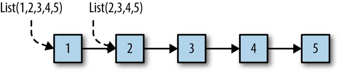
Figure 6-1. Two linked lists
Note that we created a new list from an existing list using an O(1) operation. We shared the tail with the original list and just constructed a new link from the new head element to the old list. This is our first example of an important idea in functional data structures, sharing a structure to minimize the cost of making copies. To support immutability, we need the ability to make copies with minimal cost.
Note that any other code using the original list is oblivious to the existence of the new list. Lists are immutable, so there’s no risk that the other code will be surprised by unexpected mutations happening on another thread in the code that created the new list.
It should be clear from the way linked lists are constructed that computing the size of a list is O(N), as are all other operations involving a traversal past the head of the list.
The following REPL session demonstrates constructing Lists in Scala:
// src/main/scala/progscala2/fp/datastructs/list.sc
scala> vallist1=List("Programming","Scala")
list1:Seq[String] =List(Programming, Scala)
scala> vallist2="People"::"should"::"read"::list1
list2:Seq[String] =List(People, should, read, Programming, Scala)
You can construct a list with the List.apply method, then prepend additional elements with the :: method, called “cons” (for “construct”), creating new lists. Here we used the infix notation that drops the periods and parentheses. Recall that a method name that ends with a colon (:) binds to the right. Hence x :: list is actually list.::(x).
We can also use the :: method to construct a list by prepending elements to the Nil empty list:
scala> vallist3="Programming"::"Scala"::Nil
list3:Seq[String] =List(Programming, Scala)
scala> vallist4="People"::"should"::"read"::Nil
list4:Seq[String] =List(People, should, read)
Nil is equivalent to List.empty[Nothing], where Nothing is the subtype of all other types in Scala. See The Scala Type Hierarchy for much ado about Nothing and why you can use it in this context.
Finally, you can concatenate two lists (or any sequence) together using the ++ method:
scala> vallist5=list4++list3
list5:Seq[String] =List(People, should, read, Programming, Scala)
While it’s still common to construct lists when appropriate, it is not recommended that methods be defined to take List arguments or return List values. Instead, use Seq, so that an instance of any subtype of Seq can be used, including List and Vector.
For Seq, the “cons” operator is +: instead of ::. Here is the previous session rewritten to use Seq. Note that when you use the Seq.apply method on the companion object, it constructs a List, because Seq is a trait, not a concrete class:
// src/main/scala/progscala2/fp/datastructs/seq.sc
scala> valseq1=Seq("Programming","Scala")
seq1:Seq[String] =List(Programming, Scala)
scala> valseq2="People"+:"should"+:"read"+:seq1
seq2:Seq[String] =List(People, should, read, Programming, Scala)
scala> valseq3="Programming"+:"Scala"+:Seq.empty
seq3:Seq[String] =List(Programming, Scala)
scala> valseq4="People"+:"should"+:"read"+:Seq.empty
seq4:Seq[String] =List(People, should, read)
scala> valseq5=seq4++seq3
seq5:Seq[String] =List(People, should, read, Programming, Scala)
Note that we defined an empty tail for seq3 and seq4 using Seq.empty. Most of the Scala collections have companion objects with an empty method for creating an empty instance of the collection, analogous to Nil for lists.
The sequential collections define :+ and +:. How are they different and how do you remember which is which? Just recall that the : will always be on the side of the collection, e.g., list :+ x and x +: list. So, you append an element with :+ and prepend an element with +:.
scala> valseq1=Seq("Programming","Scala")
seq1:Seq[String] =List(Programming, Scala)
scala> valseq2=seq1:+"Rocks!"
seq2:Seq[String] =List(Programming, Scala, Rocks!)
Scala only defines an immutable List. However, it also defines some mutable list types, such as ListBuffer and MutableList, when there are good reasons to use a mutable alternative.
While List is a venerable choice for a sequence, consider using immutable.Vector instead, because it provides O(1) (constant time) performance for all operations, while List is O(n) for all operations that don’t just involve accessing the head element.
Here is the previous Seq example rewritten to use Vector. Except for replacing the words Seq with Vector and changing variable names, the code is identical:
// src/main/scala/progscala2/fp/datastructs/vector.sc
scala> valvect1=Vector("Programming","Scala")
vect1:scala.collection.immutable.Vector[String] =Vector(Programming, Scala)
scala> valvect2="People"+:"should"+:"read"+:vect1
vect2:...Vector[String] =Vector(People, should, read, Programming, Scala)
scala> valvect3="Programming"+:"Scala"+:Vector.empty
vect3:...Vector[String] =Vector(Programming, Scala)
scala> valvect4="People"+:"should"+:"read"+:Vector.empty
vect4:...Vector[String] =Vector(People, should, read)
scala> valvect5=vect4++vect3
vect5:...Vector[String] =Vector(People, should, read, Programming, Scala)
However, we also get constant-time indexing.
scala> vect5(3)
res0:String = Programming
To finish our discussion of Seq, there is an important implementation issue you should know. To encourage the use of immutable collections, Predef and several other types it uses expose several immutable collection types without requiring explicit import statements or fully qualified paths in your code. Examples include List and Map.
However, Predef also brings scala.collection.Seq into scope, an exception to the rule of only exposing immutable collections. The types in scala.collection are abstractions shared by both immutable collections and by mutable collections.
Although there is a scala.collection.immutable.Seq (which subclasses scala.collection.Seq), the primary reason for exposing scala.collection.Seq instead is to make it easy to treat Java Arrays as a Seq uniformly with other collections, but they are mutable. Most other mutable collections also implement scala.collection.Seq.
Now, scala.collection.Seq does not expose any methods for mutation, but using this “default” Seq does expose a potential concurrency risk to your code, because mutable collections are not thread-safe by default, so special handling of them is required.
For example, suppose your highly concurrent library has methods that take Seq arguments, but you really only want immutable collections passed in. Using Seq opens a hole, because a client could pass you an Array, for example.
WARNING
Keep in mind that the default Seq type is actually scala.collection.Seq. So, an instance of Seq passed to your code could be mutable and therefore thread-unsafe.
The current plan for the Scala 2.12 release or a subsequent release is to change the scala.Seq alias to point to scala.collection.immutable.Seq.
Until then, if you really want to enforce usage of scala.collection.immutable.Seq instead, use the following technique (adapted from Heiko Seeberger’s blog).
We’ll use a package object, which we introduced in Package Objects. We’ll use it to define a new type alias for Seq that overrides the default definition. In fact, the scala package object is where Seq is defined to be an alias for scala.collection.Seq. We have been using the convention fp.datastructs in this section, so let’s define a package object for this package:
// src/main/scala/progscala2/fp/datastructs/package.scala
packageprogscala2.fp
packageobject datastructs {
typeSeq[+A] = scala.collection.immutable.Seq[A]
valSeq= scala.collection.immutable.Seq
}
Note that we specify the package fp first, not package fp.datastructs, followed by the package object datastructs {…} definition. The package keyword is part of the object definition. There can be only one package object per package. Finally, note the path to this file and the naming convention package.scala that are shown in the comment.
We declare a type alias and a val. Recall we discussed type declarations in Abstract Types Versus Parameterized Types. If user code includes the import statement import fp.datastructs._, then when Seq instances are declared (without a package qualifier) they will now usescala.collection.immutable.Seq instead of Scala’s default scala.collection.Seq.
The val Seq declaration puts the companion object in scope, so statements like Seq(1,2,3,4) invoke the scala.collection.immutable.Seq.apply method.
What about packages underneath fp.datastructs? If you’re implementing a package in this hierarchy, use the idiom for successive package statements we discussed in Organizing Code in Files and Namespaces:
packagefp.datastructs // Make Seq refer to immutable.Seq
packageasubpackage // Stuff in this package
packageasubsubpackage // The package I'm working on...
Consider using this idiom of defining type aliases in package objects for exposing the most important types in your own APIs.
Maps
Another common data structure is the Map, sometimes referred to as a hash, hash map, or dictionary in various languages. Maps are used to hold pairs of keys and values and they shouldn’t be confused with the map function on many data structures, although the names reflect a similar idea, associating a key with a value, or an input element with an output element.
Scala supports the special initialization syntax we saw previously:
// src/main/scala/progscala2/fp/datastructs/map.sc
scala> valstateCapitals=Map(
| "Alabama"->"Montgomery",
| "Alaska" ->"Juneau",
| "Wyoming"->"Cheyenne")
stateCapitals:scala.collection.immutable.Map[String,String] =
Map(Alabama -> Montgomery, Alaska -> Juneau, Wyoming -> Cheyenne)
scala> vallengths=stateCapitalsmap{
| kv=>(kv._1,kv._2.length)
|}
lengths:scala.collection.immutable.Map[String,Int] =
Map(Alabama -> 10, Alaska -> 6, Wyoming -> 8)
scala> valcaps=stateCapitalsmap{
| case(k,v)=>(k,v.toUpperCase)
|}
caps:scala.collection.immutable.Map[String,String] =
Map(Alabama -> MONTGOMERY, Alaska -> JUNEAU, Wyoming -> CHEYENNE)
scala> valstateCapitals2=stateCapitals+(
| "Virginia"->"Richmond")
stateCapitals2:scala.collection.immutable.Map[String,String] =
Map(Alabama -> Montgomery, Alaska -> Juneau,
Wyoming -> Cheyenne, Virginia -> Richmond)
scala> valstateCapitals3=stateCapitals2+(
| "New York"->"Albany","Illinois"->"Springfield")
stateCapitals3:scala.collection.immutable.Map[String,String] =
Map(Alaska -> Juneau, Virginia -> Richmond, Alabama -> Montgomery,
NewYork -> Albany, Illinois -> Springfield, Wyoming -> Cheyenne)
We learned previously that the key -> value idiom is actually implemented with an implicit conversion in the library. The Map.apply method expects a variable argument list of two-element tuples (pairs).
The example demonstrates two ways to define the function passed to map. Each key-value pair (tuple) is passed to this function. We can define it to take a single tuple argument or use the case match syntax discussed in Chapter 4 to decompose the tuple into a key and a value.
Finally, we see that we can add one or more new key-value pairs to the Map (creating new Maps), using +.
By the way, notice what happens if we drop the parentheses in the stateCapitals + ("Virginia" -> "Richmond") expression:
scala> stateCapitals+"Virginia"->"Richmond"
res2: (String, String) = (Map(Alabama -> Montgomery, Alaska -> Juneau,
Wyoming -> Cheyenne)Virginia,Richmond)
Wait, what? We end up with a pair of strings, (String,String). Unfortunately, we encountered Scala’s eagerness to convert something to a String so the + method can be used if no suitable alternative exists. The compiler first evaluated this subexpression, stateCapitals.toString + "Virginia". Then the -> was applied to create the tuple with “Richmond” as the second element in the tuple. That is, the resulting tuple is ("Map(Alabama -> … -> Cheyenne)Virginia", "Richmond").
WARNING
If an expression involving a + turns into a String when you don’t expect it, you probably encountered a situation where the compiler decided that the only viable way to parse the expression is to convert subexpressions to strings and add them together.
You can’t actually call new Map("Alabama" -> "Montgomery", …); it is a trait. Instead, Map.apply constructs an instance of a class that is optimal for the data set, usually based on size. For example, there are concrete maps for one, two, three, and four key-value pairs.
Unlike List, there are immutable and mutable implementations of Map: scala.collection.immutable.Map[A,B] and scala.collection.mutable.Map[A,B], respectively. You have to import the mutable version explicitly, while the immutable version is already exposed byPredef. Both implementations define + and - operators for adding and removing elements, and ++ and -- operators for adding and removing elements defined in Iterators (which could be other sets, lists, etc.).
Sets
Sets are an example of unordered collections, so they aren’t sequences. They also require each element to be unique:
// src/main/scala/progscala2/fp/datastructs/set.sc
scala> valstates=Set("Alabama","Alaska","Wyoming")
states:scala.collection.immutable.Set[String] =Set(Alabama, Alaska, Wyoming)
scala> vallengths=statesmap(st=>st.length)
lengths:scala.collection.immutable.Set[Int] =Set(7, 6)
scala> valstates2=states+"Virginia"
states2:scala.collection.immutable.Set[String] =
Set(Alabama, Alaska, Wyoming, Virginia)
scala> valstates3=states2+("New York","Illinois")
states3:scala.collection.immutable.Set[String] =
Set(Alaska, Virginia, Alabama, NewYork, Illinois, Wyoming)
Just as for Map, the scala.collection.Set trait only defines methods for immutable operations. There are derived traits for immutable and mutable sets: scala.collection.immutable.Set and scala.collection.mutable.Set, respectively. You have to import the mutable version explicitly, while the immutable version is already imported by Predef. Both define + and - operators for adding and removing elements, and ++ and -- operators for adding and removing elements defined in Iterators (which could be other sets, lists, etc.).
Traversing, Mapping, Filtering, Folding, and Reducing
The common functional collections—sequences, lists, maps, sets, as well as arrays, trees, and others—all support several common operations based on read-only traversal. In fact, this uniformity can be exploited if any “container” type you implement also supports these operations. For example, an Option is a container with zero or one elements, for None or Some, respectively.
Traversal
The standard traversal method for Scala containers is foreach, which is defined in scala.collection.IterableLike and has the following signature:
traitIterableLike[A] { // Some details omitted.
...
def foreach[U](f:A => U):Unit = {...}
...
}
Some subclasses of IterableLike may redefine the method to exploit local knowledge for better performance.
It actually doesn’t matter what the U is, the return type of the function. The output of foreach is Unit, so it’s a totally side-effecting function. Because it takes a function argument, foreach is a higher-order function, as are all the operations we’ll discuss here.
Foreach is O(N) in the number of elements. Here is an example of its use for lists and maps:
// code-examples/progscala2/fp/datastructs/foreach.sc
scala> List(1,2,3,4,5)foreach{i=>println("Int: "+i)}
Int: 1
Int: 2
Int: 3
Int: 4
Int: 5
scala>valstateCapitals=Map(
| "Alabama"->"Montgomery",
| "Alaska" ->"Juneau",
| "Wyoming"->"Cheyenne")
stateCapitals:scala.collection.immutable.Map[String,String] =
Map(Alabama -> Montgomery, Alaska -> Juneau, Wyoming -> Cheyenne)
// stateCapitals foreach { kv => println(kv._1 + ": " + kv._2) }
scala> stateCapitalsforeach{case(k,v)=>println(k+": "+v)}
Alabama:Montgomery
Alaska:Juneau
Wyoming:Cheyenne
Note that for the Map example, the A type for the function passed to foreach is actually a pair (K,V) for the key and value types. We use a pattern-match expression to extract the key and value. The alternative tuple syntax is shown in the comment.[11]
foreach is not a pure function, because it can only perform side effects. However, once we have foreach, we can implement all the other, pure operations we’ll discuss next, which are hallmarks of functional programming: mapping, filtering, folding, and reducing.
Mapping
We’ve encountered the map method before. It returns a new collection of the same size as the original collection, where each element of the original collection is transformed by a function. It is defined in scala.collection.TraversableLike and inherited by most of the collections. Its signature is the following:
traitTraversableLike[A] { // Some details omitted.
...
def map[B](f: (A) ⇒B):Traversable[B]
...
}
We saw examples of map earlier in this chapter.
Actually, this signature for map is not the one that’s in the source code. Rather, it’s the signature shown in the Scaladocs. If you look at the Scaladocs entry, you’ll see a “full signature” part at the end, which you can expand by clicking the arrow next to it. It shows the actual signature, which is this:
def map[B, That](f:A => B)(implicit bf:CanBuildFrom[Repr, B, That]):That
Recent versions of Scaladocs show simplified method signatures for some methods, in order to convey the “essence” of the method without overwhelming the reader with implementation details. The essence of a map method is to transform one collection into a new collection of the same size and kind, where the elements of type A in the original collection are transformed into elements of type B by the function.
The actual signature carries additional implementation information. That is the output kind of collection, which is usually the same as the input collection. We discussed the purpose of the implicit argument bf: CanBuildFrom in Capabilities. Its existence means we can construct a Thatfrom the output of map and the function f. It also does the building for us. Repr is the internal “representation” used to hold the elements.
Although the implicit CanBuildFrom complicates the method’s real signature (and triggers complaints on mailing lists…), without it, we would not be able to create a new Map, List, or other collection that inherits from TraversableLike. This is a consequence of using an object-oriented type hierarchy to implement the collections API. All the concrete collection types could reimplement map and return new instances of themselves, but the lack of reuse would undermine the whole purpose of using an object-oriented hierarchy.
In fact, when the first edition of Programming Scala came out, Scala v2.7.X ruled the land, and the collections API didn’t attempt to do this at all. Instead, map and similar methods just declared that they returned an Iteratable or a similar abstraction and often it was just an Array or a similar low-level type that was returned.
From now on, I’ll show the simplified signatures, to focus on the behaviors of the methods, but I encourage you to pick a collection, say List or Map, and look at the full signature for each method. Learning how to read these signatures can be a bit daunting at first, but it is essential for using the collections effectively.
There’s another interesting fact about map worth understanding. Look again at its simplified signature. I’ll just use List for convenience. The collection choice doesn’t matter for the point I’m making:
traitList[A] {
...
def map[B](f: (A) ⇒B):List[B]
...
}
The argument is a function A => B. The behavior of map is actually List[A] => List[B]. This fact is obscured by the object syntax, e.g., list map f. If instead we had a separate module of functions that take List instances as arguments, it would look something like this:
// src/main/scala/progscala2/fp/combinators/combinators.sc
objectCombinators1 {
def map[A,B](list:List[A])(f: (A) ⇒B):List[B] = list map f
}
(I’m cheating and using List.map to implement the function…)
What if we exchanged the argument lists?
objectCombinators {
def map[A,B](f: (A) ⇒B)(list:List[A]):List[B] = list map f
}
Finally, let’s use this function in a REPL session:
scala> objectCombinators{
| defmap[A,B](f:(A)⇒B)(list:List[A]):List[B]=listmapf
| }
defined module Combinators
scala> valintToString=(i:Int)=>s"N=$i"
intToString:Int => String= <function1>
scala> valflist=Combinators.map(intToString)_
flist:List[Int] =>List[String] = <function1>
scala> vallist=flist(List(1,2,3,4))
list:List[String] =List(N=1, N=2, N=3, N=4)
The crucial point is the second and third steps. In the second step, we defined a function intToString of type Int => String. It knows nothing about Lists. In the third step, we defined a new function by partial application of Combinators.map. The type of flist is List[Int] => List[String]. Therefore, we used map to lift a function of type Int => String to a function of type List[Int] => List[String].
We normally think of map as transforming a collection with elements of type A into a collection of the same size with elements of type B, using some function f: A => B that knows nothing about the collection. Now we know that we can also view map as a tool to lift an ordinary functionf: A => B to a new function flist: List[A] => List[B]. We used lists, but this is true for any container type with map.
Well, unfortunately, we can’t quite do this with the ordinary map methods in the Scala library, because they are instance methods, so we can’t partially apply them to create a lifted function that works for all instances of List, for example.
Maybe this is a limitation, a consequence of Scala’s hybrid OOP-FP nature, but we’re really talking about a corner case. Most of the time, you’ll have a collection and you’ll call map on it with a function argument to create a new collection. It won’t be that often that you’ll want to lift an ordinary function into one that transforms an arbitrary instance of a collection into another instance of the collection.
Flat Mapping
A generalization of the Map operation is flatMap, where we generate zero to many new elements for each element in the original collection. We pass a function that returns a collection, instead of a single element, and flatMap “flattens” the generated collections into one collection.
Here is the simplified signature for flatMap in TraversableLike, along with the signature for map again, for comparison:
def flatMap[B](f:A => GenTraversableOnce[B]):Traversable[B]
def map[B](f: (A) => B):Traversable[B]
Note that for map, the function f had the signature A => B. Now we return a collection, where GenTraversableOnce is an interface for anything that can be traversed at least once.
Consider this example:
// src/main/scala/progscala2/fp/datastructs/flatmap.sc
scala> vallist=List("now","is","","the","time")
list:List[String] =List(now, is, "", the, time)
scala> listflatMap(s=>s.toList)
res0:List[Char] =List(n, o, w, i, s, t, h, e, t, i, m, e)
Calling toList on each string creates a List[Char]. These nested lists are then flattened into the final List[Char]. Note that the empty string in list resulted in no contribution to the final list, while each of the other strings contributed two or more characters.
In fact, flatMap behaves exactly like calling map, followed by another method, flatten:
// src/main/scala/progscala2/fp/datastructs/flatmap.sc
scala> vallist2=List("now","is","","the","time")map(s=>s.toList)
list2:List[List[Char]] =
List(List(n, o, w), List(i, s), List(), List(t, h, e), List(t, i, m, e))
scala> list2.flatten
res1:List[Char] =List(n, o, w, i, s, t, h, e, t, i, m, e)
Note that the intermediate collection is a List[List[Char]]. However, flatMap is more efficient than making two method calls, because flatMap doesn’t create the intermediate collection.
Note that flatMap won’t flatten elements beyond one level. If our function literal returned deeply nested trees, they would be flattened only one level.
Filtering
It is common to traverse a collection and extract a new collection from it with elements that match certain criteria:
// src/main/scala/progscala2/fp/datastructs/filter.sc
scala> valstateCapitals=Map(
| "Alabama"->"Montgomery",
| "Alaska" ->"Juneau",
| "Wyoming"->"Cheyenne")
stateCapitals:scala.collection.immutable.Map[String,String] =
Map(Alabama -> Montgomery, Alaska -> Juneau, Wyoming -> Cheyenne)
scala> valmap2=stateCapitalsfilter{kv=>kv._1startsWith"A"}
map2:scala.collection.immutable.Map[String,String] =
Map(Alabama -> Montgomery, Alaska -> Juneau)
There are several different methods defined in scala.collection.TraversableLike for filtering or otherwise returning part of the original collection. Note that some of these methods won’t return for infinite collections and some might return different results for different invocations unless the collection type is ordered. The descriptions are adapted from the Scaladocs:
def drop (n : Int) : TraversableLike.Repr
Selects all elements except the first n elements. Returns a new traversable collection, which will be empty if this traversable collection has less than n elements.
def dropWhile (p : (A) => Boolean) : TraversableLike.Repr
Drops the longest prefix of elements that satisfy a predicate. Returns the longest suffix of this traversable collection whose first element does not satisfy the predicate p.
def exists (p : (A) => Boolean) : Boolean
Tests whether a predicate holds for at least one of the elements of this traversable collection. Returns true if so or false, otherwise.
def filter (p : (A) => Boolean) : TraversableLike.Repr
Selects all elements of this traversable collection that satisfy a predicate. Returns a new traversable collection consisting of all elements of this traversable collection that satisfy the given predicate p. The order of the elements is preserved.
def filterNot (p : (A) => Boolean) : TraversableLike.Repr
The “negation” of filter; selects all elements of this traversable collection that do not satisfy the predicate p…
def find (p : (A) => Boolean) : Option[A]
Finds the first element of the traversable collection satisfying a predicate, if any. Returns an Option containing the first element in the traversable collection that satisfies p, or None if none exists.
def forall (p : (A) => Boolean) : Boolean
Tests whether a predicate holds for all elements of this traversable collection. Returns true if the given predicate p holds for all elements, or false if it doesn’t.
def partition (p : (A) => Boolean): (TraversableLike.Repr, TraversableLike.Repr)
Partitions this traversable collection in two traversable collections according to a predicate. Returns a pair of traversable collections: the first traversable collection consists of all elements that satisfy the predicate p and the second traversable collection consists of all elements that don’t. The relative order of the elements in the resulting traversable collections is the same as in the original traversable collection.
def take (n : Int) : TraversableLike.Repr
Selects the first n elements. Returns a traversable collection consisting only of the first n elements of this traversable collection, or else the whole traversable collection, if it has less than n elements.
def takeWhile (p : (A) => Boolean) : TraversableLike.Repr
Takes the longest prefix of elements that satisfy a predicate. Returns the longest prefix of this traversable collection whose elements all satisfy the predicate p.
Many collection types have additional methods related to filtering.
Folding and Reducing
Let’s discuss folding and reducing together, because they’re similar. Both are operations for “shrinking” a collection down to a smaller collection or a single value.
Folding starts with an initial “seed” value and processes each element in the context of that value. In contrast, reducing doesn’t start with a user-supplied initial value. Rather, it uses one of the elements as the initial value, usually the first or last element:
// src/main/scala/progscala2/fp/datastructs/foldreduce.sc
scala> vallist=List(1,2,3,4,5,6)
list:List[Int] =List(1, 2, 3, 4, 5, 6)
scala> listreduce(_+_)
res0:Int = 21
scala> list.fold(10)(_*_)
res1:Int = 7200
scala> (listfold10)(_*_)
res1:Int = 7200
This script reduces the list of integers by adding them together, returning 21. It then folds the same list using multiplication with a seed of 10, returning 7,200.
Like reduce, the function passed to fold takes two arguments, an accumulator and an element in the initial collection. The new value for the accumulator must be returned by the function. Note that our examples either add or multiply the accumulator with the element to produce the new accumulator.
The example shows two common ways to write a fold expression, which requires two argument lists: the seed value and the function to compute the results. So, we can’t just use infix notation like we can for reduce.
However, if we really like infix notation, we can use parentheses as in the last example (list fold 10), followed by the function argument list. I’ve come to prefer this syntax myself.
It isn’t obvious why we can use parentheses in this way. To explain why it works, consider the following code:
scala> valfold1=(listfold10)_
fold1: ((Int, Int) => Int) =>Int= <function1>
scala> fold1(_*_)
res10:Int = 7200
Note that we created fold1 using partial application. Then we called it, applying the remaining argument list, (_ * _). You can think of (list fold 10) as starting a partial application, then the application is completed with the function that follows, (_ * _).
If we fold an empty collection it simply returns the seed value. In contrast, reduce can’t work on an empty collection, because there would be nothing to return. In this case, an exception is thrown:
scala> (List.empty[Int]fold10)(_+_)
res0:Int = 10
scala> List.empty[Int]reduce(_+_)
java.lang.UnsupportedOperationException:empty.reduceLeft
...
However, if you’re not sure that a collection is empty, for example because it was passed into your function as an argument, you can use optionReduce:
scala> List.empty[Int]optionReduce(_+_)
res1:Option[Int] =None
scala> List(1,2,3,4,5)optionReduce(_+_)
res2:Option[Int] =Some(15)
If you think about it, reducing can only return the closest, common parent type[12] of the elements. If the elements all have the same type, the final output will have that type. In contrast, because folding takes a seed value, it offers more options for the final result. Here is a “fold” operation that is really a map operation:
// src/main/scala/progscala2/fp/datastructs/fold-map.sc
scala> (List(1,2,3,4,5,6)foldRightList.empty[String]){
| (x,list)=>("["+x+"]")::list
|}
res0:List[String] =List([1], [2], [3], [4], [5], [6])
First, we used a variation of fold called foldRight, which traverses the collection from right to left, so that we construct the new list with the elements in the correct order. That is, the 6 is processed first and prepended to the empty list, then the 5 is prepended to that list, etc. Here, the accumulator is the second argument in the anonymous function.
In fact, all the other operations can be implemented with fold, as well as foreach. If you could only have one of the powerful functions we’re discussing, you could choose fold and reimplement the others with it.
Here are the signatures and descriptions for the various fold and reduce operations declared in scala.collection.TraversableOnce and scala.collection.TraversableLike. The descriptions are adapted from the Scaladocs:
def fold[A1 >: A](z: A1)(op: (A1, A1) ⇒ A1): A1
Folds the elements of this traversable or iterator using the specified associative binary operator op. The order in which operations are performed on elements is unspecified and may be nondeterministic. However, for most ordered collections like Lists, fold is equivalent to foldLeft.
def foldLeft[B](z: B)(op: (B, A) ⇒ B): B
Applies a binary operator op to a start value and all elements of this traversable or iterator, going left to right.
def foldRight[B](z: B)(op: (A, B) ⇒ B): B
Applies a binary operator op to all elements of this traversable or iterator and a start value, going right to left.
def /:[B](z: B)(op: (B, A) ⇒ B): B = foldLeft(z)(op)
A synonym for foldLeft. Example: (0 /: List(1,2,3))(_ + _). Most people consider the operator form /: for foldLeft to be too obscure and hard to remember. Don’t forget the importance of communicating with your readers when writing code.
def :\[B](z: B)(op: (A, B) ⇒ B): B = foldRight(z)(op)
A synonym for foldRight. Example: (List(1,2,3) :\ 0)(_ + _). Most people consider the operator form :\ for foldRight to be too obscure and hard to remember.
def reduce[A1 >: A](op: (A1, A1) ⇒ A1): A1
Reduces the elements of this traversable or iterator using the specified associative binary operator op. The order in which operations are performed on elements is unspecified and may be nondeterministic. However, for most ordered collections like Lists, reduce is equivalent toreduceLeft. An exception is thrown if the collection is empty.
def reduceLeft[A1 >: A](op: (A1, A1) ⇒ A1): A1
Applies a binary operator op to all elements of this traversable or iterator, going left to right. An exception is thrown if the collection is empty.
def reduceRight[A1 >: A](op: (A1, A1) ⇒ A1): A1
Applies a binary operator op to all elements of this traversable or iterator going right to left. An exception is thrown if the collection is empty.
def optionReduce[A1 >: A](op: (A1, A1) ⇒ A1): Option[A1]
Like reduce, but returns None if the collection is empty or Some(…) if not.
def reduceLeftOption[B >: A](op: (B, A) ⇒ B): Option[B]
Like reduceLeft, but returns None if the collection is empty or Some(…) if not.
def reduceRightOption[B >: A](op: (A, B) ⇒ B): Option[B]
Like reduceRight, but returns None if the collection is empty or Some(…) if not.
def aggregate[B](z: B)(seqop: (B, A) ⇒ B, combop: (B, B) ⇒ B): B
Aggregates the results of applying an operator to subsequent elements. This is a more general form of fold and reduce. It has similar semantics, but does not require the result to be a parent type of the element type. It traverses the elements in different partitions sequentially, using seqopto update the result, and then applies combop to results from different partitions. The implementation of this operation may operate on an arbitrary number of collection partitions, so combop may be invoked an arbitrary number of times.
def scan[B >: A](z: B)(op: (B, B) ⇒ B): TraversableOnce[B]
Computes a prefix scan of the elements of the collection. Note that the neutral element z may be applied more than once. (I’ll show you an example at the end of this section.)
def scanLeft[B >: A](z: B)(op: (B, B) ⇒ B): TraversableOnce[B]
Produces a collection containing cumulative results of applying the operator op going left to right.
def scanRight[B >: A](z: B)(op: (B, B) ⇒ B): TraversableOnce[B]
Produces a collection containing cumulative results of applying the operator op going right to left.
def product: A
Multiplies the elements of this collection. Returns the product of all elements in the collection, as long as the elements have an implicit conversion to type Numeric[A] (for example, Int, Long, Float, Double, and BigInt). The full signature of this method is actually def product[B >: A](implicit num: Numeric[B]): B. See Constraining Allowed Instances for more on using implicit conversions to constrain the use of methods to allowed types.
def mkString: String
Displays all elements of this traversable or iterator in a string. This is a custom implementation of fold used for conveniently generating a custom string from the collection. There will be no delimiter between elements in the string.
def mkString(sep: String): String
Displays all elements of this traversable or iterator in a string using the specified separator (sep) string.
def mkString(start: String, sep: String, end: String): String
Displays all elements of this traversable or iterator in a string using the specified start (prefix), sep (separator), and end (suffix) strings.
Pay careful attention to the arguments passed to the anonymous functions for various reduce, fold, and aggregate methods. For the Left methods, e.g., foldLeft, the first argument is the accumulator and the collection is traversed left to right. For the Right functions, e.g.,foldRight, the second argument is the accumulator and the collection is traversed right to left. For the methods like fold and reduce that aren’t left- or right-biased, the traversal order and which argument is the accumulator are undefined (but typically they delegate to the left-biased methods).
The reduce and fold methods can output a completely different type, based on the seed value, while the reduce methods always return the same element type or a supertype.
None of these functions will terminate for infinite collections. Also, they might return different results for different runs if the collection is not a sequence (i.e., the elements are not stored in a defined order) or the operation isn’t associative.
The aggregate method is not widely used. Because it has several “moving parts,” it is harder to understand.
The scan methods are useful for processing successive subsets of a collection. Consider the following example:
scala> vallist=List(1,2,3,4,5)
list:List[Int] =List(1, 2, 3, 4, 5)
scala> (listscan10)(_+_)
res0:List[Int] =List(10, 11, 13, 16, 20, 25)
First the seed value 10 is emitted, followed by the first element plus the seed, 11, followed by the second element plus the previous value, 11 + 2 = 13, and so on.
Finally, the three mkString methods are mentioned here because they are actually special-case versions of fold and reduce for generating a String. They are also quite handy when the default toString for a collection isn’t what you want.
Left Versus Right Traversals
Note from our listing that fold and reduce do not guarantee a particular traversal order. In contrast, foldLeft and reduceLeft traverse the element left to right, while foldRight and reduceRight traverse the elements from right to left.
Hence, any operation that must preserve the order, such as our example that converted a list of integers to a list of formatted strings, must use either foldLeft or foldRight, as appropriate.
Let’s examine the left and right forms of fold and reduce. They have important differences in behavior.
Let’s repeat a few of the examples we saw before, but now using fold, foldLeft, foldRight, reduce, reduceLeft, and reduceRight, for comparison. First, the fold examples:
scala> (List(1,2,3,4,5)fold10)(_*_)
res0:Int = 1200
scala> (List(1,2,3,4,5)foldLeft10)(_*_)
res1:Int = 1200
scala> (List(1,2,3,4,5)foldRight10)(_*_)
res2:Int = 1200
Now the reduce examples:
scala> List(1,2,3,4,5)reduce(_+_)
res3:Int = 15
scala> List(1,2,3,4,5)reduceLeft(_+_)
res4:Int = 15
scala> List(1,2,3,4,5)reduceRight(_+_)
res5:Int = 15
OK, not too exciting because the choice of method doesn’t seem to matter. The reason is the anonymous functions used, _ * _ and _ + _. They are associative and commutative.
Let’s explore this further. First, for Lists, fold just calls foldLeft; they do the same thing. That’s true for most, but not all collections. So, we’ll focus on foldLeft and foldRight. Second, the same anonymous function is used for foldLeft and foldRight, but in each case the arguments are actually reversed. For foldLeft, the first argument is the accumulator, while for foldRight, the second argument is the accumulator.
Let’s compare foldLeft and foldRight, starting with associative and commutative functions that make the purpose of the arguments explicit:
// src/main/scala/progscala2/fp/datastructs/fold-assoc-funcs.sc
scala> valfacLeft =(accum:Int,x:Int)=>accum+x
facLeft: (Int, Int) =>Int= <function2>
scala> valfacRight=(x:Int,accum:Int)=>accum+x
facRight: (Int, Int) =>Int= <function2>
scala> vallist1=List(1,2,3,4,5)
list1:List[Int] =List(1, 2, 3, 4, 5)
scala> list1reduceLeft facLeft
res0:Int = 15
scala> list1reduceRightfacRight
res1:Int = 15
The facLeft and facRight functions are associative and commutative. They differ only in how they interpret their arguments, but both have the body accum + x. To be clear, we can define a function value and pass it as an argument to a higher-order function, like reduceLeft orreduceRight.
Finally, when reduceLeft is called on list1 with facLeft passed as the anonymous function, we get the same result we get when calling reduceRight with facRight. Actually, using either anonymous function would yield the same result, because they are associative and commutative.
Let’s sketch out the actual computation that’s done in these cases. When we call reduceLeft for list1, we first pass 1 to facLeft as the accum argument (i.e., the initial seed value) and 2 as the value of x. The anonymous function facLeft then returns 1 + 2 as the next accum value,3. The next call to facLeft passes 3 as accum and 3 as x, which then returns 3 + 3 or 6. Working through the remaining steps shows us that the following computation is performed:
((((1 + 2) + 3) + 4) + 5) // = 15
In contrast, when reduceRight is used, 5 is the seed value and we process values from right to left. If you work through the steps, the computation is the following:
((((5 + 4) + 3) + 2) + 1) // = 15
Let’s reorder this expression to put the elements back in their original order. We’ll repeat the reduceLeft expression first for comparison. Note the parentheses:
((((1 + 2) + 3) + 4) + 5) // = 15 (reduceLeft case)
(1 + (2 + (3 + (4 + 5)))) // = 15 (reduceRight case)
Note how the parentheses reflect the direction of traversal. We’ll come back to these expressions shortly.
What if we use a function that is still associative, but not commutative?
scala> valfncLeft =(accum:Int,x:Int)=>accum-x
fncLeft: (Int, Int) =>Int= <function2>
scala> valfncRight=(x:Int,accum:Int)=>accum-x
fncRight: (Int, Int) =>Int= <function2>
scala> list1reduceLeft fncLeft
res0:Int = -13
scala> list1reduceRightfncRight
res1:Int = -5
To see why we get different results, let’s consider the actual computation that these functions construct.
If we repeat the preceding exercise to construct parenthesized lists of arithmetic expressions, we get the following for this example:
((((1 - 2) - 3) - 4) - 5) // = -13 (foldLeft)
((((5 - 4) - 3) - 2) - 1) // = -5 (foldRight)
(-1 + (-2 + (-3 + (-4 + 5)))) // = -5 (foldRight, rearranged)
Hence, as before, the parentheses indicate explicitly that reduceLeft processes the list elements from the left, while reduceRight processes the list elements from the right.
To be clear that the functions fncLeft and fncRight are associative, recall that x - y is equivalent to x + -y, which can be written -y + x without changing the results:
((((1 - 2) - 3) - 4) - 5) // original
((((1 + -2) + -3) + -4) + -5) // changing x - y to x + -y
(1 + (-2 + (-3 + (-4 + -5)))) // demonstrating associativity
Finally, let’s consider what happens when we use functions that are neither associative nor commutative. We’ll use functions that construct Strings:
scala> valfnacLeft =(x:String,y:String)=>s"($x)-($y)"
scala> valfnacRight=(x:String,y:String)=>s"($y)-($x)"
scala> vallist2=list1map(_.toString) // Make a list of Strings
scala> list2reduceLeft fnacLeft
res2:String = ((((1)-(2))-(3))-(4))-(5)
scala> list2reduceRightfnacRight
res3:String = ((((5)-(4))-(3))-(2))-(1)
scala> list2reduceRightfnacLeft
res4:String = (1)-((2)-((3)-((4)-(5))))
Note again the different results from using fnacLeft and fnacRight. Be sure you understand how the resulting strings are produced.
Tail Recursion Versus Traversals of Infinite Collections
It turns out that foldLeft and reduceLeft have an important advantage over foldRight and reduceRight: the left traversals are tail-call recursive, so they can benefit from Scala’s tail-call optimization.
To see this, recall the expressions we constructed previously for adding the elements of a list:
((((1 + 2) + 3) + 4) + 5) // = 15 (reduceLeft case)
(1 + (2 + (3 + (4 + 5)))) // = 15 (reduceRight case)
Recall that a tail call must be the last operation in an iteration. For each line in the reduceRight sequence, the outermost addition (1 + …) can’t be performed until all of the nested additions finish, so the operation can’t be converted to a loop and it isn’t tail recursive. Recall that for lists we have to process the elements from head to tail, because of the way lists are constructed. In contrast, for the reduceLeft case, we can add the first two elements, then the third, then the fourth, etc. In other words, we can convert it to a loop, because it’s tail recursive.
Another way to see this is to implement our own foldLeft and foldRight for Seqs:
// src/main/scala/progscala2/fp/datastructs/fold-impl.sc
// Simplified implementation. Does not output the actual collection type
// that was input as Seq[A].
def reduceLeft[A,B](s:Seq[A])(f:A => B):Seq[B] = {
@annotation.tailrec
def rl(accum:Seq[B], s2:Seq[A]):Seq[B] = s2 match {
case head +: tail => rl(f(head) +: accum, tail)
case_=> accum
}
rl(Seq.empty[B], s)
}
def reduceRight[A,B](s:Seq[A])(f:A => B):Seq[B] = s match {
case head +: tail => f(head) +: reduceRight(tail)(f)
case_=>Seq.empty[B]
}
val list =List(1,2,3,4,5,6)
reduceLeft(list)(i => 2*i)
// => List(12, 10, 8, 6, 4, 2)
reduceRight(list)(i => 2*i)
// => List(2, 4, 6, 8, 10, 12)
These implementations don’t attempt to construct the actual subclass of the input Seq for the output. The Scala collections implementations use the CanBuildFrom technique we discussed previously. Otherwise, they follow the classic model for implementing a left or right traversal using recursion.
You should learn these two patterns well enough to always remember the behaviors and trade-offs of left versus right traversal and recursion, even though in practice you’ll almost always use Scala’s built-in functions instead of writing your own.
Because we are processing a Seq, we should normally work with the elements left to right. It’s true that Seq.apply(index: Int) returns the element at position index (counting from zero). However, for a linked list, this would require an O(N) traversal for each call to apply, yielding anO(N2) algorithm rather than O(N), which we want. So, the implementation of foldRight “suspends” prefixing the value to the rest of the new Seq until the recursive invocation of foldRight returns. Hence, foldRight is not tail recursive.
For foldLeft, we use a nested function rl to implement the recursion. It carries along an accum argument that accumulates the new Seq[B]. When we no longer match on head +: tail, we’ve hit the empty tail Seq, at which point we return accum, which has the completed Seq[B]we’ll return. When we make a recursive call to rl, it is the last thing we do (the tail call), because we prepend the new element to accum before passing its updated value to rl. Hence, foldLeft is tail recursive.
In contrast, when we hit the end of the input Seq in foldRight, we return an empty Seq[B] and then the new elements are prefixed to it as we pop the stack.
Finally, note the order of the output elements, which are different. It may surprise you at first that the left recursion returns a list that effectively reverses the input elements, but this is just an artifact of how sequences are constructed by prepending items to another sequence. Try rewriting both functions to work with Vectors. You can use the same case match clauses, but append the elements to the new vector, rather than prepend them. The output vector from your new foldLeft will have the elements in the same order as the input, while the output of foldRight will now reverse the order.
So why have both kinds of recursion? If you’re not worried about stack overflow, a right recursion might be the most natural fit for the operation you are doing. We saw that our foldRight for sequences keeps the elements in the same order. We could call reverse on the output offoldLeft, but that means two traversals of a collection, not just one. That could be expensive for very large collections.
However, there is one advantage of a right recursion over a left recursion. Consider the case where you have a potentially infinite stream of data coming in. You can’t conceivably put all that data into a collection in memory, but perhaps you only need to process the first N elements, for someN, and then discard the rest. The library’s Stream type is designed for this purpose. Stream is lazy, which means that it only evaluates its tail on demand (but it evaluates the head eagerly, which is sometimes inconvenient).
By “evaluate,” I mean that the only possible way to define an infinite stream in computing is to use some function that will produce values forever. That function could be reading from an input channel, like a socket, such as the Twitter “firehose,” or a large file. Or it could be a function that generates a sequence of numbers. We’ll see an example of the latter in a moment.
Now suppose we defined an infinite collection where the infinite function just generates random numbers. Most of Scala’s collections are strict or eager, meaning that if we attempted to define a collection with this function, it would immediately consume all available memory while trying to build up this collection in memory.
On the other hand, a lazy stream would just call the random function once for the head, then wait until a client asked for subsequent values from the tail of the stream.
Let’s consider an interesting example of an infinite Stream of numbers, the Fibonacci sequence.
Recall that a Fibonacci number fib(n) is defined as follows (ignoring negative numbers):
f(n) =
0 if n = 0
1 if n = 1
f(n-1) + f(n-2) otherwise
Like any good recursion, n equals 0 or 1 provides the termination condition we need, in which case f(n) = n. Otherwise, f(n) = f(n-1) + f(n-2).
Now consider this definition using Streams:
// src/main/scala/progscala2/fp/datastructs/fibonacci.sc
scala> importscala.math.BigInt
scala> valfibs:Stream[BigInt]=
| BigInt(0)#::BigInt(1)#::fibs.zip(fibs.tail).map(n=>n._1+n._2)
scala> fibstake10foreach(i=>print(s"$i "))
0 1 1 2 3 5 8 13 21 34
Using the equivalent of the “cons” operation, #::, for Stream, we construct the first two values of the sequence eagerly for the special case of n equals 0 and 1, then we define the rest of the stream with a recursive definition. It is right-recursive, but we’ll only take the first n elements and discard the rest.
Note that we are both defining fibs and defining the tail portion using fibs itself: fibs.zip(fibs.tail).map(…). This tail expression pairs up all elements of fibs with the successor elements. For example, we have tuple elements like (f(2), f(3)), (f(3), f(4)), etc. going on to infinity, but we don’t actually evaluate these expressions eagerly until the user asks for values. Note that the tuples are then mapped to an integer, the sum of their values, which is the next f(n) value!
The last line uses take to evaluate the first ten numbers in the sequence. (Eager collections also have the take method.) We must compute the tail eight times to get a total of ten numbers. Then we loop over them with foreach and print them, one per line.
This is a very clever and powerful definition of a recursive sequence, taken from the Stream Scaladoc page. Make sure you understand what it’s doing. It helps to play with the pieces of the expression to understand what each one does and then work out the first several values by hand.
It’s important to note that the structure of fibs is very similar to our implementation of foldRight, f(0) + f(1) + tail. Because it is effectively a right recursion, we can stop evaluating tail when we have as many head elements as we want. In contrast, trying to construct a left recursion that is also lazy is not possible, because it would look conceptually like this: f(0 + f(1 + f(tail)). (Compare our implementation of foldLeft). Hence, a right recursion lets us work with infinite, lazy streams, truncating them appropriately, while a left recursion does not.
NOTE
Left recursions are tail recursive. Right recursions can handle infinite, lazy streams with truncation.
However, note that some of the types that implement foldRight and reduceRight on sequences actually reverse the sequence first, then invoke foldLeft or reduceLeft, respectively. For example, collection.TraversableOnce provides this implementation for most Seqs. This allows users to perform right-biased operations in a tail-recursive way, although with the extra overhead of reversing the sequence first.
Combinators: Software’s Best Component Abstractions
When object-oriented programming went mainstream in the late ’80s and early ’90s, there was great hope that it would usher in an era of reusable software components, even an industry of component libraries. It didn’t really work out that way, except in limited cases, like the windowing APIs of various platforms.
Why did this era of reusable components not materialize? There are certainly many factors, but the fundamental reason is that appropriate, generative source code or binary interoperability protocols never materialized that would be the basis of these components. It’s a paradox that the richness of object APIs actually undermined modularization into reusable components.
In the larger world, component models that succeeded are all based on very simple foundations. Digital integrated circuits (ICs) plug into buses with 2n signaling wires, each of which is Boolean, either on or off. Upon the foundation of this extremely simple protocol, an industry was born with the most explosive growth of any industry in human history.
HTTP is another successful example of a “component model.” Services interact through a narrow, well-defined interface, involving a handful of message types and a very simple standard for message content.
In both cases, higher-level protocols were built upon simple foundations, but these foundations enabled composition to create, to generate, more complex structures. In digital circuits, some binary patterns are interpreted as CPU instructions, others as memory addresses, and others as data values. REST, data formats like JSON, and other higher-level standards are built upon the foundation of HTTP.
When you look at a city, at first it looks like most buildings are unique, completely customized creations. In fact, standards are behind the unique veneers: electric power, water and sewage, standard conventions for room dimensions, standard furnishings, and these buildings are surrounded by standard roads holding cars that have their own hierarchy of standards.
Object-oriented programming never established fundamental, generative standards. Within each language community, the fundamental unit of composition is the object (with or without a class “template”). Yet objects are not fundamental enough. Every developer invents a new “standard” for a Customer type. No two teams can agree what fields and behaviors the Customer type should have, because each team needs different data and computations for scenarios related to customers. Something more fundamental than an object is needed.
Attempts to standardize components across language and process boundaries also came up short. Models like CORBA were far from simple. Most defined a binary (versus source) standard. This made interoperability very brittle, subject to version hell. It wasn’t the choice of binary versus source standardization that was the problem. It was the complexity of the binary standard that led to failure.
In contrast, think about the examples we studied in this chapter. We started with a small set of collections, Lists, Vectors, Maps, etc., that all share a set of operations in common, most of which are defined on the Seq abstraction (trait). Most of our examples used Lists, but that was an arbitrary choice.
Except for the utility method foreach, the operations were all pure, higher-order functions. They had no side effects and they took other functions as arguments to do the custom work for filtering or transforming each element from the original collection. Such higher-order functions are related to the mathematical concept of combinators from Combinatory Logic.
We can sequence together these combinator functions to build up nontrivial behavior with relatively little code. We can separate data from the behavior we need to implement for particular problems. This is in opposition to the normal approach of object-oriented programming, which combines data and behavior. It’s more typical to create ad hoc implementations of domain logic inside custom classes. We’ve seen a more productive way in this chapter. This is why the chapter started with the Alan J. Perlis quote.
Let’s finish this discussion with a final example, a simplified payroll calculator:
// src/main/scala/progscala2/fp/combinators/payroll.sc
caseclassEmployee (
name:String,
title:String,
annualSalary:Double,
taxRate:Double,
insurancePremiumsPerWeek:Double)
val employees =List(
Employee("Buck Trends", "CEO", 200000, 0.25, 100.0),
Employee("Cindy Banks", "CFO", 170000, 0.22, 120.0),
Employee("Joe Coder", "Developer", 130000, 0.20, 120.0))
// Calculate weekly payroll:
val netPay = employees map { e =>
val net = (1.0 - e.taxRate) * (e.annualSalary / 52.0) -
e.insurancePremiumsPerWeek
(e, net)
}
// "Print" paychecks:
println("** Paychecks:")
netPay foreach {
case (e, net) => println(f" ${e.name+':'}%-16s ${net}%10.2f")
}
// Generate report:
val report = (netPay foldLeft (0.0, 0.0, 0.0)) {
case ((totalSalary, totalNet, totalInsurance), (e, net)) =>
(totalSalary + e.annualSalary/52.0,
totalNet + net,
totalInsurance + e.insurancePremiumsPerWeek)
}
println("\n** Report:")
println(f" Total Salary: ${report._1}%10.2f")
println(f" Total Net: ${report._2}%10.2f")
println(f" Total Insurance: ${report._3}%10.2f")
This script prints the following:
** Paychecks:
Buck Trends: 2784.62
Cindy Banks: 2430.00
Joe Coder: 1880.00
** Report:
Total Salary: 9615.38
Total Net: 7094.62
Total Insurance: 340.00
We could have implemented this logic in many ways, but let’s consider a few of the design choices.
First, although this section criticized object-oriented programming as a component model, OOP is still quite useful. We defined an Employee type to hold the fields for each employee. In a real application, we would load this data from a database.
Instead, what if we just use tuples instead of a custom type? You might try rewriting the code this way and compare the two versions. Using Employee and the names it provides for the different fields makes it easier to reason about the code. Meaningful names is an old principle of good software design. Although I’ve emphasized the virtues of fundamental collections, functional programming does not say that custom types are bad. As always, design trade-offs should be carefully considered.
However, Employee is anemic. It is a structure with minimal behavior. In classic object-oriented design, we might add a lot of behavior to Employee to help with the payroll calculation or other domain logic. I believe the design chosen here provides optimal separation of concerns. It’s also so concise that the maintenance burden is small if the structure of Employee changes and this code has to change.
Note also that the logic was implemented using a small script, rather than a large application combining many classes defined over many files. Of course, this is a toy example, but hopefully you can see how nontrivial applications don’t necessarily require large code bases.
There is a counterargument for using a dedicated type, the overhead of constructing instances. Here, this overhead is unimportant. What if we have billions of records? We’ll return to this question when we explore Big Data in Chapter 18.
What About Making Copies?
Let’s finish this chapter by considering a practical problem. Making copies of functional collections is necessary to preserve immutability, but suppose I have a Vector of 100,000 items and I need a copy with the item at index 8 replaced. It would be terribly inefficient to construct a completely new, 100,000-element Vector.
Fortunately, we don’t have to pay this penalty, nor must we sacrifice immutability. The secret is to realize that 99,999 elements are not changing. If we can share the parts of the original Vector that aren’t changing, while representing the change in some way, then creating the new vector can still be very efficient. This idea is called structure sharing.
If other code on a different thread is doing something different with the original vector, it is unaffected by the copy operation, because the original vector is not modified. In this way, a “history” of vectors is preserved, as long as there are references to one or more older versions. No version will be garbage-collected until there are no more references to it.
Because this history is maintained, a data structure that uses structure sharing is called a persistent data structure.
Our challenge is to select an implementation data structure that lets us expose Vector semantics (or the semantics of another data structure), while providing efficient operations that exploit structure sharing. Let’s sketch the underlying data structure and how the copy operation works. We won’t cover all the details in depth. For more information start with the Wikipedia page on persistent data structures.
The tree data structure with a branching factor of 32 is used. The branching factor is the maximum number of child nodes each parent node is allowed to have and it means that search and modification operations are O(log32(N)), effectively a constant for even large values of N!
Figure 6-2 shows an example for Vector(1,2,3,4,5). We’ll use just two or three child nodes for legibility.
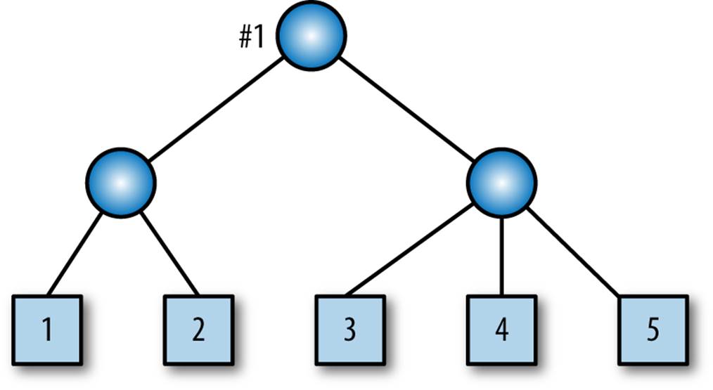
Figure 6-2. A Vector represented as a tree
When you reference the vector, you’re actually referencing the root of this tree, marked by #1. As an exercise, you might work through how operations like accessing a particular element by its index, map, flatMap, etc., would work on a tree implementation of a Vector.
Now suppose we want to insert 2.5 between 2 and 3. To create a new copy, we don’t mutate the original tree, but instead create a new tree. Figure 6-3 shows what happens when we add 2.5 between 2 and 3.
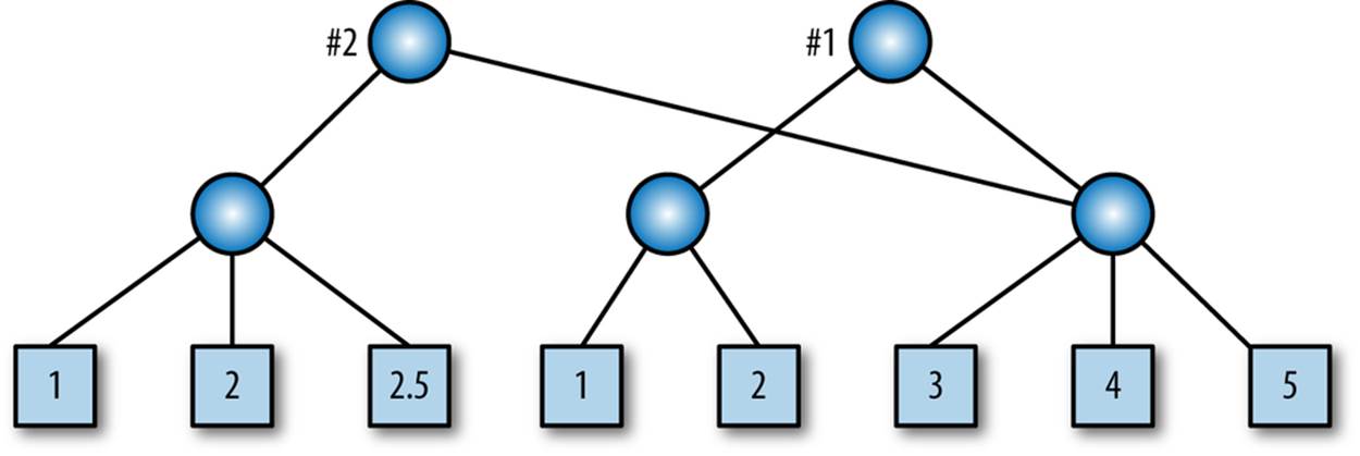
Figure 6-3. Two states of a Vector, before and after element insertion
Note that the original tree (#1) remains, but we have created a new root (#2) and new nodes between it and the child holding the new element. A new left subtree was created. With a branching factor of 32, we will have to copy up to 32 child references per level, but this number of copy operations is far less than the number required for all references in the original tree. Special handling is required when you need to add an element to a node that already has 32 elements.
Deletion and other operations work similarly. A good textbook on data structures will describe the standard algorithms for tree operations.
Therefore, it is possible to use large, immutable data structures, if their implementations support an efficient copy operation. There is extra overhead compared to a mutable vector, where you can simply modify an entry in place very quickly. Ironically, that doesn’t mean that object-oriented and other procedural programs are necessarily simpler and faster.
Because of the dangers of mutability, it’s common for classes to wrap collections they hold in accessor methods, which increase the code footprint, testing burden, etc. Worse, if the collection itself is exposed through a “getter” method, it’s common to create defensive copies, where a copy of the collection is returned, rather than the original, so that a client can’t modify the internal state of the object by modifying the collection outside the object’s control. Because collection implementations in nonfunctional languages often have inefficient copy operations, the net effect can be less efficient programs than corresponding functional programs.
Immutable collections can not only be efficient, but they eliminate the need for all this extra code to defend against unwanted mutation.
There are other kinds of functional data structures that are optimized for efficient copying, optimized for modern hardware, such as minimizing cache misses, and other purposes. Many of these data structures were invented as alternatives to mutable data structures that are commonly discussed in classic textbooks on data structures and algorithms. For more on functional data structures, see Purely Functional Data Structures by Chris Okasaki and Pearls of Functional Algorithm Design by Richard Bird (both by Cambridge University Press), and Algorithms: A Functional Programming Approach, by Fethi Rabhi and Guy Lapalme (Addison-Wesley).
Recap and What’s Next
We discussed the basic concepts of FP and argued for their importance for solving modern problems in software development. We saw how the fundamental collections and their common higher-order functions, combinators, yield concise, powerful, modular code.
Typical functional programs are built on this foundation. At the end of the day, all programs input data, perform transformations on it, then output the results. Much of the “ceremony” in typical programs just obscures this essential purpose.
Fortunately, traditional object-oriented languages have added many of these features. Most now support combinators on collections. Java 8 brings anonymous functions (called lambdas) to Java and the collections have been enhanced with higher-order functions.
For another, gentle introduction to FP aimed at programmers with OOP backgrounds, see Functional Programming for the Object-Oriented Programmer by Brian Marick (Leanpub). If you want to convince your Java developer friends that FP is worth their attention, consider my shortIntroduction to Functional Programming for Java Developers (O’Reilly).
Functional Programming in Scala, by Paul Chiusano and Rúnar Bjarnason (Manning Publications), is an excellent, in-depth introduction to functional programming using Scala.
To practice using combinators, see Phil Gold’s “Ninety-Nine Scala Problems” webpage.
Next, we’ll return to for comprehensions and use our new knowledge of FP to understand how for comprehensions are implemented, how we can implement our own data types to exploit them, and how the combination of for comprehensions and combinator methods yield concise, powerful code. Along the way, we’ll deepen our understanding of functional concepts.
We’ll return to more advanced features of functional programming in Chapter 16 and we’ll dive into more of the implementation details of Scala’s collections in Chapter 12.
[10] There’s a joke in the Haskell community that they have delayed success until the last possible minute.
[11] The anonymous function with the case clause is actually defining a PartialFunction, but it’s really total because it will successfully match on all the inputs in this case.
[12] Also called the least upper bound or LUB.