Systems Programming: Designing and Developing Distributed Applications, FIRST EDITION (2016)

Chapter 2. The Process View

Abstract

This chapter examines systems and communication within systems from the process viewpoint. The process is the central theme around which the concepts of modular systems and multiple communicating systems are presented and explained. Process scheduling and management are examined for both real-time and non-real-time applications. Communication is treated as input to and output from processes. The way that interprocess communication is facilitated, and the way that communication behavior may interact with process scheduling behavior, is discussed. Multithreading is introduced and discussed in terms of ensuring responsiveness of processes. The use of timers within processes to provide control and generate periodic tasks is investigated.

Keywords

Process

Scheduling

Threads

Thread scheduling

Sockets

Input stream

Output stream

Pipe

Process states

Workload characteristics

Deadline

Interprocess communication

Program

Real time scheduling

Priority

Preemption

Operating system

2.1 Rationale and Overview

The process is the ultimate endpoint of communication in distributed systems. Within a particular system or application, multiple processes execute as separate entities, scheduled by the operating system. However, for these processes to act cooperatively and coherently to solve application problems, they need to communicate. Understanding the nature of processes and the way they interact with the operating system is a key prerequisite to designing systems of processes that communicate to build higher-level structures and thus solve application-level problems of distributed systems.

The abbreviation IO will be used when discussing input and output in generic contexts.

2.2 Processes

This section examines the nature of processes and the way in which they are managed by operating systems. In particular, the focus is on the way in which input and output (IO) from devices is mapped onto the IO steams of a process and the way in which interprocess communication (IPC) is achieved with pipelines.

2.2.1 Basic Concepts

It is first necessary to introduce the basic concepts of processes and their interaction with systems. This sets the scene for the subsequent deeper investigation.

We start with the definition of a program.

A program is a list of instructions together with structure and sequence information to control the order in which the instructions are carried out.

Now let us consider the definition of a process.

A process is the running instance of a program.

This means that when we run (or execute) a program, a process is created (see below).

The most important distinction between a program and a process is that a program does not do anything; rather, it is a description of how to do something. When a process is created, it will carry out the instructions of the related program.

A set of instructions that are supplied with home-assembly furniture are a useful analogy to a computer program. They provide a sequenced (numbered) set of individual steps describing how to assemble the furniture. The furniture will not be assembled just because of the existence of the instructions. It is only when someone actually carries out the instructions, in the correct order, that the furniture gets built. The act of following the instructions step by step is analogous to the computer process.

Another important relationship between a program and a process is that the same program can be run (executed) many times, each time giving rise to a unique process. We can extend the home-assembly furniture analogy to illustrate; each set of furniture is delivered with a copy of the instructions (i.e., the same “program”), but these are instantiated (i.e., the instructions are carried out) at many different times and in different places, possibly overlapping in time such that two people may be building their furniture at the same time—unbeknownst to each other.

2.2.2 Creating a Process

The first step is to write a program that expresses the logic required to solve a particular problem. The program will be written in a programming language of your choice, for example, C++ or C#, enabling you to use a syntax that is suitably expressive to represent high-level ideas such as reading input from a keyboard device, manipulating data values, and displaying output on a display screen.

A compiler is then used to convert your human-friendly high-level instructions into low-level instructions that the microprocessor understands (thus the low-level instruction sequence that the compiler generates is called machine code). Things can go wrong at this point in two main ways. Syntax errors are those errors that break the rules of the language being used. Examples of syntax errors include misspelled variable names or keywords, incorrect parameter types, or incorrect numbers of parameters being passed to methods and many other similar mistakes (if you have done even a little programming, you can probably list at least three more types of syntax error that you have made yourself). These errors are automatically detected by the compiler and error messages are provided to enable you to locate and fix the problems. Thus, there should be no ongoing issues arising from syntax once you get the code to compile.

Semantic errors are errors in the presentation of your logic. In other words, the meaning as expressed by the logic of the program code is not the intended meaning of the programmer. These errors are potentially far more serious because generally, there will be no way for the compiler to detect them. For example, consider that you have three integer variables A, B, and C and you intend to perform the calculation C = A – B but you accidentally type C = B – A instead! The compiler will not find any errors in your code as it is syntactically correct, and the compiler certainly has no knowledge of the way your program is supposed to work and does not care what actual value or meaning is ascribed to variables A, B, and C. Semantic errors must be prevented by careful design and discipline during implementation and are detected by vigilance on the part of the developer, and this must be supported by a rigorous testing regime.

Let us assume we now have a logically correct program that has been compiled and stored in a file in the form of machine code that the microprocessor hardware can understand. This type of file is commonly referred to as an executable file, because you can “execute” (run) it by providing its name to the operating system. Some systems identify such files with a particular filename extension, for example, the Microsoft Windows system uses the extension “.exe”.

It is important to consider the mechanism for executing a program. A program is a list of instructions stored in a file. When we run a program, the operating system reads the list of instructions and creates a process that comprises an in-memory version of the instructions, the variables used in the program, and some other metadata concerning, for example, which instruction is to be executed next. Collectively, this is called the process image and the metadata and variables (i.e., the changeable parts of the image) are called the process state, as the values of these describe, and are dependent on, the state of the process (i.e., the progress of the process through the set of instructions, characterized by the specific sequence of input values in this run-instance of the program). The state is what differentiates several processes of the same program. The operating system will identify the process with a unique Process IDentifier (PID). This is necessary because there can be many processes running at the same time in a modern computer system and the operating system has to keep track of the process in terms of, among other things, who owns it, how much processing resource it is using, and which IO devices it is using.

The semantics (logic) represented by the sequence of actions arising from the running of the process is the same as that expressed in the program. For example, if the program adds two numbers first and then doubles the result, the process will perform these actions in the same order and will provide an answer predictable by someone who knows both the program logic and the input values used.

Consider the simplest program execution scenario as illustrated in Figure 2.1.

FIGURE 2.1 Pseudocode for a simple process.

Figure 2.1 shows the pseudocode for a very simple process. Pseudocode is a way of representing the main logical actions of the program, in a near-natural language way, yet still unambiguously, that is independent of any particular programming language. Pseudocode does not contain the full level of detail that would be provided if the actual program were provided in a particular language such as C++, C#, or Java, but rather is used as an aid to explain the overall function and behavior of programs.

The program illustrated in Figure 2.1 is a very restricted case. The processing itself can be anything you like, but with no input and no output, the program cannot be useful, because the user cannot influence its behavior and the program cannot signal its results to the user.

A more useful scenario is illustrated in Figure 2.2.

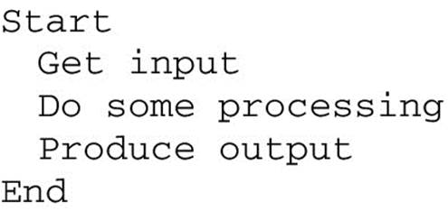
FIGURE 2.2 Pseudocode of a simple process with input and output.

This is still conceptually very simple, but now, there is a way to steer the processing to do something useful (the input) and a way to find out the result (the output).

Perhaps the easiest way to build a mental picture of what is happening is to assume that the input device is a keyboard and the output device is the display screen. We could write a program Adder with the logic shown in Figure 2.3.

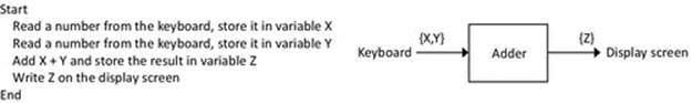
FIGURE 2.3 Two aspects of the process, the pseudocode and a block representation, which shows the process with its inputs and outputs.

If I type the number 3 and then the number 6 (the two input values), the output on the display screen will be 9.

More accurately, a process gets its input from an input stream and sends its output to an output stream. The process when running does not directly control or access devices such as the keyboard and display screen; it is the operating system's job to pass values to and from such devices. Therefore, we could express the logic of program Adder as shown in Figure 2.4.

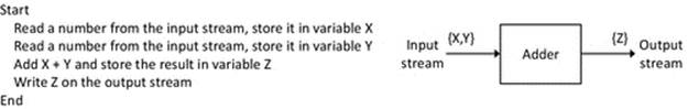
FIGURE 2.4 The Adder process with its input and output streams.

When the program runs, the operating system can (by default) map the keyboard device to the input stream and the display screen to the output stream.

Let's define a second program Doubler (see Figure 2.5).

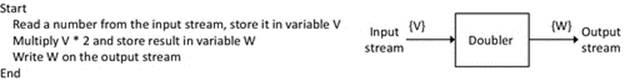
FIGURE 2.5 The Doubler process; pseudocode and representation with input and output streams.

We can run the program Doubler, creating a process with the input stream connected to the keyboard and the output stream connected to the display screen. If I type the number 5 (the input), the output on the screen will be 10.

The concept of IO streams gives rise to the possibility that the IO can be connected to many different sources or devices and does not even have to involve the user directly. Instead of the variable W being displayed on the screen, it could be used as the input to another calculation, in another process. Thus, the output of one process becomes the input to another. This is called a pipeline (as it is a connector between two processes, through which data can flow) and is one form of IPC. We use the pipe symbol | to represent this connection between processes. The pipeline is implemented by connecting the output stream of one process to the input stream of another. Notice that it is the operating system that actually performs this connection, and not the processes themselves.

The Adder and Doubler processes could be connected such that the output of Adder becomes the input to Doubler, by connecting the appropriate steams. In this scenario, the input stream for process Adder is mapped to the keyboard, and the output stream for process Doubler is mapped to the display screen. However, the output stream for Adder is now connected to the input stream for Doubler, via a pipeline.

Using the pipe notation, we can write Adder | Doubler.

This is illustrated in Figure 2.6.

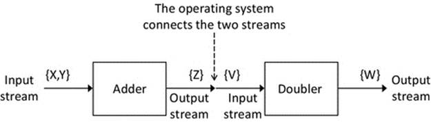
FIGURE 2.6 The Adder and Doubler processes connected by a pipe.

If I type the number 3 and then the number 6 (the two input values), the output on the display screen will be 18. The output of process Adder is still 9, but this is not exposed to the outside world (we can call this a partial result as the overall computation is not yet complete). Process Doubler takes the value 9 from process Adder and doubles it, giving the value 18, which is then displayed on the screen.

We have reached the first practical activity of this chapter. The activities are each set out in the form of an experiment, with identified learning outcomes and a method to follow.

I have specifically taken the approach of including carefully scoped practical tasks that the reader can carry out as they read the text because the learning outcomes are better reinforced by actually having the hands-on experience. The practical tasks are designed to reinforce the theoretical concepts introduced in the main text. Many of the practical tasks also support and encourage your own exploration by changing parameters or configuration to ask what-if questions.

The presentation of the activities also reports expected outcomes and provides guidance for reflection and in some cases suggestions for further exploration. This is so that readers who are unable to run the experiments at the time of reading can still follow the text.

The first Activity P1 provides an opportunity to investigate IPC using pipes.

The example in Activity P1 is simple, yet nevertheless extremely valuable. It demonstrates several important concepts that are dealt with in later sections:

Activity P1

Exploring Simple Programs, Input and Output Streams, and Pipelines

Prerequisites

The instructions below assume that you have previously performed Activity I1 in Chapter 1. This activity places the necessary supplemental resources on your default disk drive (usually C:) in the directory SystemsProgramming. Alternatively, you can manually copy the resources and locate them in a convenient place on your computer and amend the instructions below according to the installation path name used.

Learning Outcomes

This activity illustrates several important concepts that have been discussed up to this point:

1. How a process is created as the running instance of a program by running the program at the command line

2. How the operating system maps input and output devices to the process

3. How two processes can be chained together using a pipeline

Method

This activity is carried out in three steps:

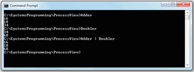
1. Run the Adder.exe program in a command window. Navigate to the ProcessView subfolder of the SystemsProgramming directory and then execute the Adder program by typing Adder.exe followed by the Enter key. The program will now run as a process. It waits until two numbers have been typed (each one followed by the Enter key) and then adds the numbers and displays the result, before exiting.

2. Run the Doubler.exe program in the same manner as for the Adder.exe program in step 1. The process waits for a single number to be typed (followed by the Enter key) and then doubles the number and displays the result, before exiting.

3. Run the Adder and Doubler programs in a pipeline. The goal is to take two numbers input by the user and to display double the sum of the two numbers. We can write this formulaically as:

where X and Y are the numbers entered by the user and Z is the result that is displayed. For example, if X = 16 and Y = 18, the value of Z will be 68.
The command-line syntax to achieve this is Adder | Doubler.
The first process will wait for two numbers to be typed by the user. The output of the Adder process will be automatically mapped onto the input of the Doubler process (because the | was used), and the Doubler process will double the value it receives, which is then output to the display screen.

The image below shows the results when the three steps above are followed:

Expected Outcome

For each of the first two steps, you will see that the program was executed as a process that follows the logic of the program (see the source code in file Adder.cpp and also Doubler.cpp). Notice that by default, the operating system automatically mapped the keyboard as the input device and the display screen as the output device although this was not specified in the program. You will also see how the operating system remaps the input and output streams of the processes when the pipeline is used. The individual programs are used as building blocks to construct more complex logic.

Reflection

1. Study the source code of the two programs and read the built-in comments.

2. Think about the different roles of the programmer who wrote the two programs, the operating system, and the user who types the command line and provides the input and how each influence the end result. It is important to realize that the overall behavior seen in this activity is a result of a combination of the program logic, the operating system control of execution, and the user's input data.

1. Processes can communicate; for example, the output from one process can become the input to another process.

2. In order for processes to communicate, there needs to be a mechanism to facilitate this. In the simple scenario here, the operating system facilitates the IPC by using the pipeline mechanism as a connector between the output stream of one process and the input stream of the other.

3. Higher-level functionality can be built up from simpler logic building blocks. In the example, the externally visible logic is to add two numbers and double the result; the user sees the final result on the display screen and does not need to know how it was achieved. This is the concept of modularity and is necessary to achieve sophisticated behavior in systems while keeping the complexity of individual logical elements to manageable levels.

2.3 Process Scheduling

This section examines the role the operating system plays in managing the resources of the system and scheduling processes.

A process is “run” by having its instructions executed in the central processing unit (CPU). Traditionally, general-purpose computers have had a single CPU, which had a single core (the core is the part that actually executes a process). It is becoming common in modern systems to have multiple CPUs and/or for each CPU to have multiple cores. Since each core can run a single process, a multiple core system can run multiple processes at the same time. For the purpose of limiting the complexity of the discussion in this book, we shall assume the simpler, single-core architecture, which means that only a single process can actually execute instructions at any instant (i.e., only one process is running at a time).

The most fundamental role of an operating system is to manage the resources of the system. The CPU is the primary resource, as no work can be done without it. Thus, an important aspect of resource management is controlling usage of the CPU (better known as process scheduling). Modern operating systems have a special component, the scheduler, which is specifically responsible for managing the processes in the system and selecting which one should run at any given moment. This is the most obvious and direct form of interaction between processes and the operating system, although indirect interaction also arises through the way in which the operating system controls the other resources that a particular process may be using.

Early computers were very expensive and thus were shared by large communities of users. A large mainframe computer may have been shared across a whole university, for example. A common way to accommodate the needs of many users was to operate in “batch mode.” This required that users submit their programs to be run into a “batch queue” and the system operators would oversee the running of these programs one by one. In terms of resource management, it is very simple; each process is given the entire resources of the computer, until either the task completes or a run-time limit may be imposed. The downside of this approach is that a program may be held in the queue for several hours. Many programs were run in overnight batches, which meant that the results of the run were not available until the next day.

The Apollo space missions to the moon in the 1960s and 1970s provide an interesting example of the early use of computers in critical control applications. The processing power of the onboard Apollo Guidance Computer¹ (AGC) was a mere fraction of that of modern systems, often likened simplistically to that of a modern desktop calculator, although through sophisticated design, the limited processing power of this computer was used very effectively. The single-core AGC had a real-time scheduler, which could support eight processes simultaneously; each had to yield if another higher-priority task was waiting. The system also supported timer-driven periodic tasks within processes. This was a relatively simple system by today's standards, although the real-time aspects would still be challenging from a design and test viewpoint. In particular, this was a closed system in which all task types were known in advance and simulations of the various workload combinations could be run predeployment to ensure correctness in terms of timing and resource usage. Some modern systems are closed in this way, in particular embedded systems such as the controller in your washing machine or the engine management system in your car (see below). However, the general-purpose computers that include desktop computers, servers in racks, smartphones, and tablets are open and can run programs that the user chooses, in any combination; thus, the scheduler must be able to ensure efficient use of resources and also to protect the quality of service (QoS) requirements of tasks in respect to, for example, responsiveness.

Some current embedded systems provide useful examples of a fixed-purpose computer. Such a system only performs a design-time specified function and therefore does not need to switch between multiple applications. Consider, for example, the computer system that is embedded into a typical washing machine. All of the functionality has been predecided at design time. The user can provide inputs via the controls on the user interface, such as setting the wash temperature or the spin speed, and thus configure the behavior but cannot change the functionality. There is a single program preloaded

Activity P2

Examine List of Processes on the Computer (for Windows Operating Systems)

Prerequisites

Requires a Microsoft Windows operating system.

Learning Outcomes

1. To gain an understanding of the typical number of and variety of processes present on a typical general-purpose computer

2. To gain an appreciation of the complexity of activity in multiprocessing environment

3. To gain an appreciation of the need for and importance of scheduling

Method

This activity is performed in two parts, using two different tools to inspect the set of processes running on the computer.

Part 1

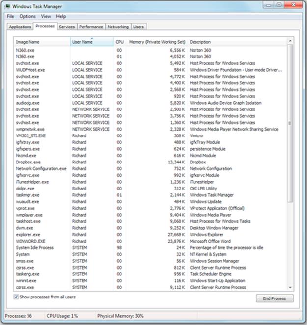
Start the Task Manager by pressing the Control, Alt, and Delete keys simultaneously and select “Start Task Manager” from the options presented. Then, select the Applications tab and view the results, followed by the Processes tab, and also view the results. Make sure the “Show processes for all users” checkbox is checked, so that you see everything that is present. Note that this procedure may vary across different versions of the Microsoft operating systems.

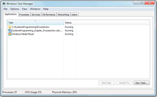
Expected Outcome for Part 1

You will see a new window that contains a list of the applications running on the computer, or a list of the processes present, depending on which tab is selected. Examples from my own computer (which has the Windows 7 Professional operating system) are shown. The first screenshot shows the list of applications, and the second screenshot shows the list of processes.

Part 2

Explore the processes present in the system using the TASKLIST command run from a command window. This command gives a different presentation of information than that provided by the Task Manager. Type TASKLIST /? to see the list of parameters that can be used. Explore the results achieved using some of these configuration parameters to see what can you find out about the processes in the system and their current state.

Reflection

You will probably have a good idea which applications are running already (after all, you are the user), so the list of applications will be of no surprise to you. In the examples from my computer, you can see that I was editing a chapter from this book while listening to a CD via the media player application.

However, you will probably see a long list of processes when selecting the Processes tab. Look closely at these processes; is this what you expected? Do you have any idea what all these are doing or why they are needed?

Note that many of the processes running are “system” processes that are either part of the operating system or otherwise related to resource management; device drivers are a good example of this.

Note especially the “System Idle Process,” which in the example above “runs” for 98% of the time. This pseudoprocess runs when no real processes are ready to run, and the share of CPU time it gets is often used as an inverse indication of the overall load on the computer.

into these systems, and this program runs as the sole process. Many embedded systems platforms have very limited resources (especially in terms of having a small memory and low processing speed) and thus cannot afford the additional overheads of having an operating system.

Now, bearing in mind how many processes are active on your computer, consider how many processes can run at any given time. For older systems, this is likely to be just 1. For newer systems, which are “dual core,” for example, the answer is 2, or 4 if it is “quad core.” Even if we had perhaps 32 cores, we would typically still have more processes than cores.

Fundamentally, the need for scheduling is that there tend to be more processes active on a computer than there are processor units, which can deal with them. If this is the case, then something has to arbitrate; this is one of the most important things the operating system does.

2.3.1 Scheduling Concepts

Several different scheduling techniques (algorithms) have been devised. These have different characteristics, the most important differentiator being the basis on which tasks are selected to run.

Given that generally there are more processes than processors, the processes can be said to be competing for the processor. To put it another way, the processes each have work to do and it is important that they eventually complete their work, but at any given moment, some of these may be more important, or urgent than others. The scheduler must ensure that wherever possible, the processor is always being used by a process, so that resource is not wasted. The performance of the scheduler is therefore most commonly discussed in terms of the resulting efficiency of the system, and this is measured in terms of the percentage of time that the processing unit is kept busy. “Keeping the processor busy” is commonly expressed as the primary goal of the scheduler. Figures 2.7 and 2.8illustrate this concept of efficiency.

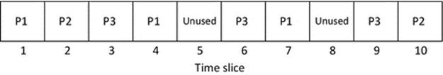
FIGURE 2.7 Schedule A uses 8 out of 10 timeslots (a system with three processes).

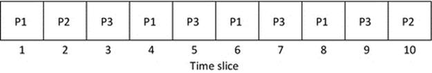
FIGURE 2.8 Schedule B uses 10 out of 10 timeslots (a system with three processes).

As shown in Figure 2.7, schedule A uses 8 of the 10 processor timeslots and is thus 80% efficient. The two timeslots that were not used are lost, that resource cannot be reclaimed. Another way to think of this situation is that this system is performing 80% of the work that it could possibly do, so is doing work at 80% of its maximum possible rate.

Figure 2.8 shows the ideal scenario in which every timeslot is used and is thus 100% efficient. This system is performing as much work as it could possibly do, so is operating its maximum possible rate.

2.3.1.1 Time Slices and Quanta

A preemptive scheduler will allow a particular process to run for a short amount of time called a quantum (or time slice). After this amount of time, the process is placed back in the ready queue and another process is placed into the run state (i.e., the scheduler ensures that the processes take turns to run).

The size of a quantum has to be selected carefully. Each time the operating system makes a scheduling decision, it is itself using the processor. This is because the operating system comprises one or more processes and it has to use system processing time to do its own computations in order to decide which process to run and actually move them from state to state; this is called context switching and the time taken is the scheduling overhead. If the quanta are too short, the operating system has to perform scheduling activities more frequently, and thus, the overheads are higher as a proportion of total system processing resource.

On the other hand, if the quanta are too long, the other processes in the ready queue must wait longer between turns, and there is a risk that the users of the system will notice a lack of responsiveness in the applications to which these processes belong.

Figure 2.9 illustrates the effects of quanta size on the total scheduling overheads. Part (a) of the figure shows the situation that arises with very short quanta. The interleaving of processes is very fine, which is good for responsiveness. This means that the amount of time a process must wait before its next quanta of run time is short and thus the process appears to be running continuously to an observer such as a human user who operates on a much slower timeline. To understand this aspect, consider, as analogy, how a movie works. Many frames per second (typically 24 or more) are flashed before the human eye, but the human visual system (the eye and its brain interface) cannot differentiate between the separate frames at this speed and thus interpret the series of frames as a continuous moving image. If the frame rate is reduced to less than about 12 frames per second, a human can perceive them as a series of separate flashing images. In processing systems, shorter quanta give rise to more frequent scheduling activities, which absorbs some of the processing resource. The proportion of this overhead as a fraction of total processing time available increases as the quanta get smaller, and thus, the system can do less useful work in a given time period, so the optimal context switching rate is not simply the fastest rate that can be achieved.

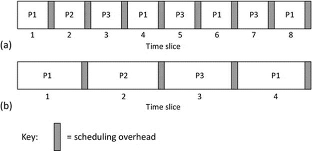
FIGURE 2.9 Quantum size and scheduling overheads.

In part (b) of Figure 2.9, the quanta have been increased to approximately double the size of those shown in part a. This increases the coarseness of the process interleaving and could impact on the responsiveness of tasks, especially those that have deadlines or real-time constraints associated with their work. To get an initial understanding of the way this can materialize, imagine a user interface that has a jerky response, where it seems to freeze momentarily between dealing with your input. This jerky response could be a symptom that the process that controls the user interface is not getting a sufficient share of processing time or that the processing time is not being shared on a sufficiently fine-grained basis. Despite the impacts on task responsiveness that can arise with having larger quanta, they are more efficient because the operating system's scheduling activities occur less frequently, thus absorbing a smaller proportion of overall processing resource; for the scenario shown, the scheduling overhead for system (b) is half that of system (a).

Choosing the size of the time quantum is an optimization problem between on the one hand the overall processing efficiency and on the other hand the responsiveness of tasks. To some extent, the ideal value depends on the nature of the applications running in the system. Real-time systems (i.e., ones that have applications with a time-based functionality or dependency, such as streaming video where each frame must be processed with strict timing requirements) generally need to use shorter quanta to achieve finer interleaving and thus ensure the internal deadlines of applications are not missed. Specific scheduling issues arising from deadlines or real-time constraints of processes will be discussed in more detail later.

Activity P3

Examining Scheduling Behavior with Real Processes—Introductory

Prerequisites

The instructions below assume that you have obtained the necessary supplemental resources as explained in Activity P1.

Learning Outcomes

This activity explores the way in which the scheduler facilitates running several processes at the same time:

1. To understand that many processes can be active in a system at the same time

2. To understand how the scheduler creates an illusion that multiple processes are actually running at the same time, by interleaving them on a small timescale

3. To gain experience of command-line arguments

4. To gain experience of using batch files to run applications

Method

This activity is carried out in three parts, using a simple program that writes characters to the screen on a periodic basis, to illustrate some aspects of how the scheduler manages processes.

Part 1

1. Run the PeriodicOutput.exe program in a command window. Navigate to the “ProcessView” subfolder and then execute the PeriodicOutput program by typing PeriodicOutput.exe followed by the Enter key. The program will now run as a process. It will print an error message because it needs some additional information to be typed after the program name. Extra information provided in this way is termed “command-line arguments” and is a very useful and important way of controlling the execution of a program.

2. Look at the error message produced. It is telling us that we must provide two additional pieces of information, which are the length of the time interval (in ms) between printing characters on the display screen and the character that will be printed at the end-of-each time interval.

3. Run the PeriodicOutput.exe program again, this time providing the required command-line parameters.
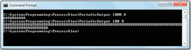
For example, if you type PeriodicOutput 1000 A, the program will print a series of A's, one each second (1000 ms).
As another example, if you type PeriodicOutput 100 B, the program will print a series of B's, one every 1/10th of a second.
Experiment with some other values. Notice that the program will always run for 10 s (10,000 ms) in total, so the number of characters printed will always be 10,000 divided by the first parameter value. Examine the source code for this program (which is provided as part of the supplemental resources) and relate the program's behavior to the instructions.

Expected Outcome for Part 1

The screenshot below shows the output for a couple of different parameter settings. So far, we have only run one process at a time.

Part 2

1. We will now run several copies of the PeriodicOutput.exe program at the same time. To do this, we shall use a batch file. A batch file is a script containing a series of commands to be executed by the system; for the purpose of this activity, you can think of it as a metaprogram that allows us to specify how programs will be executed. The batch file we shall use is called “PeriodicOutput_Starter.bat”. You can examine the contents of this file by typing “cat PeriodicOutput_Starter.bat” at the command prompt. You will see that this file contains three lines of text, each of which is a command that causes the operating system to start a copy of the PeriodicOutput.exe program, with slightly different parameters.

2. Run the batch file by typing its name, followed by the Enter key. Observe what happens.

Expected Outcome for Part 2

You should see the three processes running simultaneously, evidenced by the fact that their outputs are interleaved such that you see an “ABCABC” pattern (perfect interleaving is not guaranteed and thus the pattern may vary). The screenshot below shows the typical output you should get.

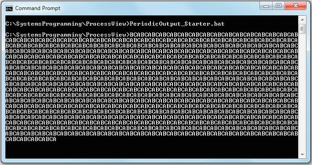
The batch file sets the intervals between printing characters to 20 ms for each of the three processes. This is on a similar scale to the size of a typical scheduling quantum and yields quite a regular interleaving (which arises because the three processes spend a relatively long time “sleeping” between their brief single-character-at-a-time output activity, giving the scheduler plenty of time to manage other activities in the system).

Part 3

Experiment with different settings by editing the batch file (use a simple text editor such as Notepad, and do not use a word processor as this may add special characters, which confuse the command interpreter part of the operating system). Try changing the time interval, or adding a few extra processes. In particular, try a shorter character printing interval for the three processes, such as 5 ms. The faster the rate of activity in the three processes, the less likely it becomes that the scheduler will achieve the regular interleaving we saw in part 2 above. Because the computer has other processes running (as we saw in Activity P2), we may not see a perfect interleaved pattern, and if we run the batch file several times, we should expect slightly different results each time; it is important that you realize why this is.

Reflection

You have seen that the simple interleaving achieved by running three processes from a batch file can lead to a regular pattern when the system is not stressed (i.e., when the processes spend most of their time blocked because they perform IO, between short episodes of running and becoming blocked once again). Essentially, there is sufficient spare CPU capacity in this configuration that each process gets the processing time it needs, without spending long in the ready state.

However, depending on the further experimentation you carried out in part 3, you will probably have found that the regularity of the interleaving in fact depends on the number of, and behavior of, other processes in the system. In this experiment, we have not stated any specific requirement of synchrony between the three processes (i.e., the operating system has no knowledge that a regular interleaving pattern is required), so irregularity in the pattern would be acceptable.

In addition to gaining an understanding of the behavior of scheduling, you should have also gained a level of competence with regard to configuring and running processes, the use of command-line arguments and batch files, and an understanding of the effects of the scheduler.

An interesting observation is that while over the past couple of decades central processor operating speeds (the number of CPU cycles per second) have increased dramatically, the typical range of scheduling quantum sizes has remained generally unchanged. One main reason for this is that the complexity of systems and the applications that run on them have also increased at high rates, requiring more processing to achieve their rich functionality. The underlying trade-off between responsiveness (smaller quantum size) and low overheads (larger quantum size) remains, regardless of how fast the CPU operates. Quantum sizes in modern systems are typically in the range of about 10 ms to about 200 ms, although smaller quanta (down to about 1 ms) are used on very fast platforms. A range of quantum sizes can be used as a means of implementing process priority; this works on the simple basis that higher-priority processes should receive a greater share of the processing resource available. Of course, if processes are IO-intensive, they get blocked when they perform IO regardless of priority.

Another main factor why quantum sizes have not reduced in line with technological advances is that human perception of responsiveness has not changed. It is important from a usability viewpoint that interactive processes respond to user actions (such as typing a key or moving the mouse) in a timely way, ideally to achieve the illusion that the user's application is running continuously, uninterrupted, on the computer. Consider a display-update activity; the behind-the-scenes processing requirement has increased due, for example, to higher-resolution displays and more complex windowing user-interface libraries. This means that a display update requires more CPU cycles in modern systems than in simpler, earlier systems.

For interactive processes, a quantum must be sufficiently large that the processing associated with the user's request can be completed. Otherwise, once the quantum ends, the user's process will have to wait, while other processes take turns, introducing delay to the user's process. In addition, as explained earlier, a smaller quantum size incurs a higher level of system overhead due to scheduling activity. So although CPU cycle speed has increased over time, the typical scheduling quantum size has not.

2.3.1.2 Process States

This section relates primarily to preemptive scheduling schemes, as these are used in the typical systems that are used to build distributed systems.

If we assume that there is only a single processor unit, then only one process can use the processor at any moment. This process is said to be running, or in the run state. It is the scheduler's job to select which process is running at a particular time and, by implication, what to do with the other processes in the system.

Some processes that are not currently running will be able to run; this means that all the resources they need are available to them, and if they were placed in the run state, they would be able to perform useful work. When a process is able to run, but not actually running, it is placed in the ready queue. It is thus said to be ready, or in the ready state.

Some processes are not able to run immediately because they are dependent on some resource that is not available to them. For example, consider a simple calculator application that requires user input before it can compute a result. Suppose that the user has entered the sequence of keys 5 x; clearly, this is an incomplete instruction and the calculator application must wait for further input before it can compute 5 times whatever second number the user enters. In this scenario, the resource in question is the keyboard input device, and the scheduler will be aware that the process is unable to proceed because it is waiting for input. If the scheduler were to let this process run, it would be unable to perform useful work immediately; for this reason, the process is moved to the blockedstate. Once the reason for waiting has cleared (e.g., the IO device has responded), the process will be moved into the ready queue. In the example described above, this would be when the user has typed a number on the keyboard.

Taking the Adder program used in Activity P1 as an example; consider the point where the process waits for each user input. Even if the user types immediately, say, perhaps one number each second, it takes 2 s for the two numbers to be entered; and this makes minimal allowance for user thinking time, which tends to be relatively massive compared to the computational time needed to process the data entered.

The CPU works very fast relative to human typing speed; even the slowest microcontroller used in embedded systems executes 1 million or more instructions per second.² The top-end mobile phone microprocessor technology (at the time of writing) contains four processing cores, which each operate at 2.3 GHz, while a top-end desktop PC microprocessor operates at 3.6-4.0 GHz, also with four processing cores. These figures provide an indication of the amount of computational power that would be lost if the scheduler allowed the CPU to remain idle for a couple of seconds while a process such as Adder is waiting for input. As discussed earlier, scheduling quanta are typically in the range of 10-200 ms, which given the operating speed of modern CPUs represents a lot of computational power.

The three process states discussed above form the basic set required to describe the overall behavior of a scheduling system generically, although some other states also occur and will be introduced later. The three states (running, ready, and blocked) can be described in a state-transition diagram, so-called because the diagram shows the allowable states of the system and the transitions that can occur to move from one state to another. A newly created process will be placed initially in the ready state.

Figure 2.10 shows the three-state transition diagram. You should read this diagram from the perspective of a particular process. That is, the diagram applies individually to each process in the system; so, for example, if there are three processes {A, B, C}, we can describe each process as being in a particular state at any given moment. The same transition rules apply to all processes, but the states can be different at any given time.

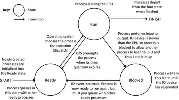
FIGURE 2.10 The three-state state transition diagram.

The transitions shown are the only ones allowable. The transition from ready to running occurs when the process is selected to run, by the operating system; this is known as dispatching. The various scheduling algorithms select the next process to run based on different criteria, but the general essence is that the process selected either has reached the top of the ready queue because it has been waiting longest or has been elevated to the top because it has a higher priority than others in the queue.

The transition from running to ready occurs when the process has used up its time quantum. This is called preemption and is done to ensure fairness and to prevent starvation; this term is used to describe the situation where one process hogs the CPU, while another process is kept waiting, possibly indefinitely.

The transition from running to blocked occurs when the process has requested an IO operation and must wait for the slower (slow with respect to the CPU) IO subsystem to respond. The IO subsystem could be a storage device such as a hard magnetic disk drive or an optical drive (CD or DVD), or it could be an output device such as a printer or video display. The IO operation could also be a network operation, perhaps waiting for a message to be sent or received. Where the IO device is a user-input device such as a mouse or keyboard, the response time is measured in seconds or perhaps tenths of a second, while the CPU in a modern computer is capable of executing perhaps several thousand million instructions in 1 s (this is an incredible amount). Thus, in the time between a user typing keys, the CPU can perform many millions of instructions, thus highlighting the extent of wastage if the process were allowed to hog the CPU while idle.

The transition from blocked to ready occurs when the IO operation has completed. For example, if the reason for blocking was waiting for a user keystroke, then once the keystroke has been received, it will be decoded and the relevant key-code data provided on the input stream of the process.³ At this point, the process is able to continue processing, so it is moved to the ready state. Similarly, if the reason for blocking was waiting for a message to arrive over a network connection, then the process will be unblocked once a message has been received⁴ and placed into a memory buffer accessible to the process (i.e., the operating system moves the message into the process' memory space).

Note that when a process is unblocked, it does not reenter the running state directly. It must go via the ready state.

As explained above, blocking and unblocking are linked to actual events in the process' behavior and in the response of IO subsystems, respectively. To illustrate this, consider what takes place when a process writes to a file on a hard disk. A hard disk is a “block device”—this means that data are read from, and written to, the disk in fixed-size blocks. This block-wise access is because a large fraction of the access time is taken up by the read/write head being positioned over the correct track where the data are to be written and waiting for the disk to rotate to the correct sector (portion of a track) where the data are to be written. It would thus be extremely inefficient and require very complex control systems if a single byte were written at a time. Instead a block of data, of perhaps many kilobytes, is read or written sequentially once the head is aligned (the alignment activity is termed “seeking” or “head seek”). Disk rotation speeds and head movement speeds are very slow relative to the processing speeds of modern computers. So, if we imagine a process that is updating a file that is stored on the disk, we can see that there would be a lot of delays associated with the disk access. In addition to the first seek, if the file is fragmented across the disk, as is common, then each new block that is to be written requires a new seek. Even after a seek is complete, there is a further delay (in the context of CPU-speed operations) as the actual speed at which data are written onto the disk or read from it is also relatively very slow. Each time the process were ready to update a next block of data, it would be blocked by the scheduler. Once the disk operation has completed, the scheduler would move the process back into the ready queue. When it enters the running state, it will process the next section of the file, and then, as soon as it is ready to write to the disk again, it is blocked once more. We would describe this as an IO-intensive task and we would expect it to be regularly blocked before using up its full-time slices. This type of task would spend a large fraction of its time in the blocked state, as illustrated in Figure 2.11.

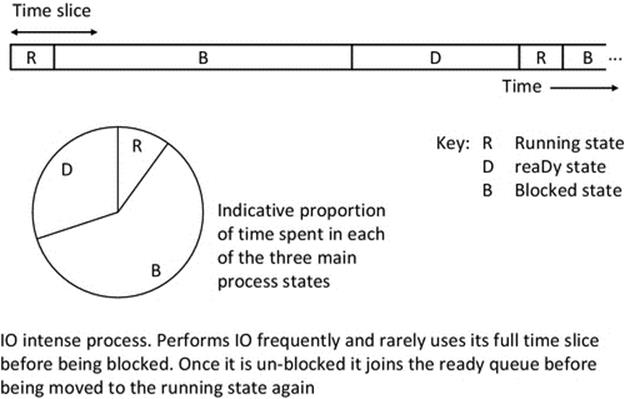
FIGURE 2.11 Run-time behavior illustration for an IO-intensive process.

Figure 2.11 illustrates the process state sequence for a typical IO-intensive process. The actual ratios shown are indicative, because they depend on the specific characteristics of the process and the host system (including the mix of other tasks present, which affects the waiting time).

The above example concerning access to a secondary storage system such as a disk drive raises a key performance issue, which must be considered during design of low-level application behavior, which affects not only its performance but also its robustness. Data held in memory while the program is running are volatile; this means that if the process crashes or the power is lost, the data are also lost. Secondary storage such as a magnetic hard disk is nonvolatile, or “persistent,” and thus will preserve the data after the process ends and even after the computer is turned off. Clearly, there is a conflict between ultimate performance and ultimate robustness, because the time-cost overheads of the most robust approach of writing data to disk every time there is a change are generally not tolerable from a performance point of view. This is a good example of a design trade-off to reach an appropriate compromise depending on the specific requirements of the application.

Compute-intensive processes tend to use their full-time slice and are thus preempted by the operating system to allow another process to do some work. The responsiveness of compute-intensive processes is thus primarily related to the total share of the system resources each gets. For example, if a compute-intensive process were the only process present, it would use the full resource of the CPU. However, if three CPU-intensive tasks were competing in a system, the process state behavior of each would resemble that shown in Figure 2.12.

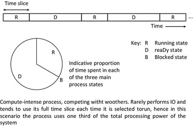
FIGURE 2.12 Run-time behavior illustration for a compute-intensive process competing with two similar processes.

One further example is provided to ensure the behavior is clear. If a compute-intensive process competes with four similar processes, each will account for one-fifth of the total computing resource available, as illustrated in Figure 2.13.

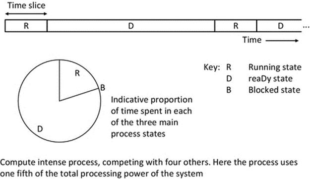
FIGURE 2.13 Run-time behavior illustration for a compute-intensive process competing with four similar processes.

2.3.1.3 Process Behavior

IO-Intensive Processes

Some processes perform IO frequently and thus are often blocked before using up their quantum; these are said to be IO-intensive processes. An IO-intensive program not only could be an interactive program where the IO occurs between a user and the process (via, e.g., the keyboard and display screen)

Activity P4

Examining Scheduling Behavior with Real Processes—Competition for the CPU

Prerequisites

The instructions below assume that you have obtained the necessary supplemental resources as explained in Activity P1.

Learning Outcomes

This activity explores the way in which the scheduler shares the CPU resource when several competing processes are CPU-intensive:

1. To understand that the CPU resource is finite

2. To understand that the performance of one process can be affected by the other processes in the system (which from its point of view constitute a background workload with which it must compete for resources).

Method

This activity is carried out in four parts and uses a CPU-intensive program, which, when running as a process, performs continual computation without doing any IO and thus never blocks. As such, the process will always fully use its time slice.

Part 1 (Calibration)

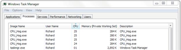
1. Start the Task Manager as in Activity P2 and select the “Processes” tab. Sort the display in order of CPU-use intensity, highest at the top. If there are no compute-intensive tasks present, the typical highest CPU usage figure might be about 1%, while many processes that have low activity will show as using 0% of the CPU resource. Leave the Task Manager window open, to the side of the screen.

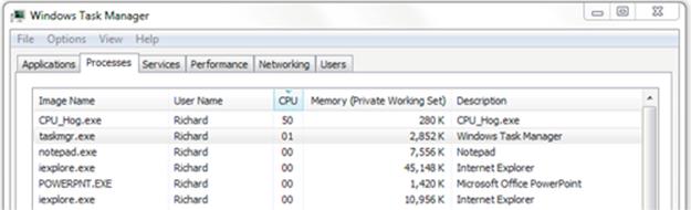
2. Run the CPU_Hog.exe program in a command window. Navigate to the “ProcessView” subfolder of the SystemsProgramming folder and then execute the CPU_Hog program by typing CPU_Hog.exe followed by the Enter key. The program will now run as a process. Examine the process statistics in the Task Manager window while the CPU_Hog process runs.
The screenshot below shows that the CPU_Hog takes as much CPU resource as the scheduler gives it, which in this case is 50%.

3. Run the CPU_Hog process again, and this time, record how long it takes to run, using a stopwatch. The program performs a loop a large fixed number of times, each time carrying out some computation. The time taken will be approximately the same each time the process is run, on a particular computer, as long as the background workload does not change significantly. It is necessary that you time it on your own computer to get a baseline for the subsequent experiments in this activity and that you do this without any other CPU-intensive processes running. Timing accuracy to the nearest second is adequate. As a reference, it took approximately 39 s on my (not particularly fast) computer.

Part 2 (Prediction)

1. Taking into account the share of CPU resource used by a single instance of the CPU_Hog, what do you think will happen if we run two instances of this program at the same time? How much share of the CPU resource do you think each copy of the program will get?

2. Based on the amount of time that it took for a single instance of the CPU_Hog to run, how long will each copy take to run if two copies are running at the same time?

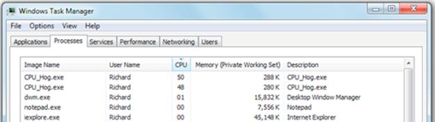
3. Now, use the batch file named “CPU_Hog_2Starter.bat” to start two copies of CPU_Hog at the same time. Use the Task Manager window to observe the share of CPU resource that each process gets, and don't forget to also measure the run time of the two processes (when they have completed, you will see them disappear from the list of processes).

The screenshot below shows that each CPU_Hog process was given approximately half of the total CPU resource. Is this what you expected?

Expected Outcome for Part 2

In my experiment, the processes ran for approximately 40 s, which is what I had expected, on the basis that each process had very slightly less than 50% (on average) of the CPU resource, which was essentially the same as the single process had had in part 1. The fact that the processes took very slightly longer to run than the single process had taken is important. This slight difference arises because the other processes in the system, while relatively inactive, do still use some processing resource and, importantly, the scheduling activity itself incurs overheads each time it switches between the active processes. These overheads were absorbed when the CPU was idle for nearly 50% of the time but show up when the resource is fully utilized.

Part 3 (Stressing the System)

It would not satisfy my inquisitive nature to leave it there. There is an obvious question that we should ask and try to answer: If a single instance of CPU_Hog takes 50% of the CPU resource when it runs and two copies of CPU_Hog take 50% of the CPU resource each, what happens when three or even more copies are run at the same time?

1. Make your predictions—for each of the three processes, what will be the share of CPU resource? And what will be the run time?

2. Use the batch file named “CPU_Hog_3Starter.bat” to start three copies of CPU_Hog at the same time. As before, use the Task Manager window to observe the share of CPU resource that each process gets, and also remember to measure the run time of the three processes (this may get trickier, as they might not all finish at the same time, but an average timing value will suffice to get an indication of what is happening).

The screenshot below shows the typical results I get.

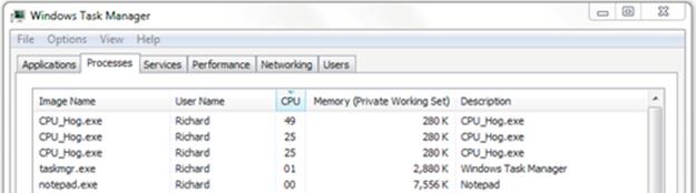
Expected Outcome for Part 3

Interestingly, the first process still gets 50% of the CPU resource and the other two share the remaining 50%. Before the experiment, I had expected that they would get 33% of the resource each. There are almost certainly other schedulers out there for which that would have been the case; but with distributed systems, you won't always know or control which computer your process will run on, or which scheduler will be present, or the exact run-time configuration including workload, so this experiment teaches us to be cautious when predicting run-time performance even in a single system, let alone in heterogeneous distributed systems.

Coming back to our experiment, this result means that the first process ends sooner than the other two. Once the first process ends, the remaining two are then given 50% of the CPU resource each, so their processing rate has been speeded up. I recorded the following times: first process, 40 s; second and third processes, approximately 60 s. This makes sense; at the point where the first process ends, the other two have had half as much processing resource each and are therefore about halfway through their task. Once they have 50% of the CPU resource each, it takes them a further 20 s to complete the remaining half of their work—which is consistent.

Part 4 (Exploring Further)

I have provided a further batch file “CPU_Hog_4Starter.bat” to start four copies of CPU_Hog at the same time. You can use this with the same method as in part three to explore further.

The screenshot below shows the behavior on my computer.

In this case, each process used approximately 25% of the CPU resource and each took approximately 80 s to run—which is consistent with the earlier results.

Reflection

This experiment illustrates some very important aspects of scheduling and of the way in which the behavior of the scheduler and the behavior of the processes interact. This includes the complexities of predicting run times and the extent to which the behavior of schedulers may be sensitive to the mix of processes in the system.

Firstly, we see that the CPU resource is finite and must be shared among the processes in the system. We also see that as some processes complete, the share of resource can be reallocated to the remaining processes. It is also important to realize that a process will take a predictable amount of CPU run time to execute. However, because the process gets typically less than 100% of the CPU resource, its actual execution time (its time in the system, including when it is in the ready queue) is greater than its CPU run time, and the overall execution time is dependent on the load on the system—which in general is continually fluctuating. These experiments have scratched the surface of the complexity of scheduling but provide valuable insight into the issues concerned and equip us with the skills to explore further. You can devise further empirical experiments based on the tools I have provided (e.g., you can edit the batch files to fire off different combinations of programs), or you can use the Operating Systems Workbench scheduling simulations that support flexible experimentation over a wide range of conditions and process combinations and also allow you to decide which scheduler to use. The introductory scheduling simulation provides configurations with three different schedulers and workload mixes of up to five processes of three different types. The advanced scheduling simulation supports an additional scheduling algorithm and facilitates configuration of the size of the CPU scheduling quantum and also the device latency for IO-intensive processes. The workbench will be introduced later in the chapter.

but also may perform its IO to other devices including disk drives and the network—for example, it may be a server process that receives requests from a network connection and sends responses back over the network.

Examples of IO-intensive programs are shown in the pseudocode in Figure 2.14 (user-interactive IO), Figure 2.15 (disk-based IO), and Figure 2.16 (network-based IO).

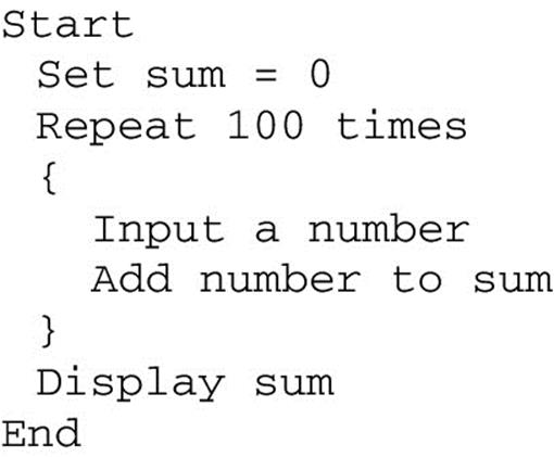
FIGURE 2.14 The Summer IO-intensive (interactive) program (computes the sum of 100 numbers).

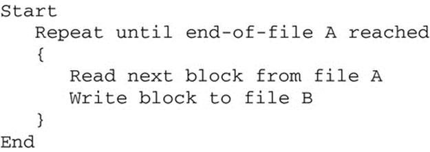
FIGURE 2.15 The FileCopy IO-intensive (disk access) program (copy from one file to another).

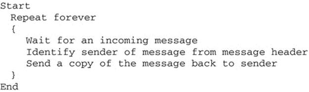
FIGURE 2.16 NetworkPingService IO-intensive (network communication) program (echo back a received message to the sender).

Figure 2.14 shows the pseudocode of an interactive IO-intensive process that spends a very large proportion of its time waiting for input. The time to perform the add operation would be much less than a millionth of a second, so if the user enters numbers at a rate of 1 per second, the program could spend greater than 99.9999% of its time waiting for input.

Figure 2.15 shows pseudocode for a disk IO-intensive program that spends most of its time waiting for a response from the hard disk; each loop iteration performs two disk IO operations.

Figure 2.16 shows pseudocode for a network IO-intensive program that spends most of its time waiting for a message to arrive from the network.

Figures 2.14–2.16 provide three examples of processes that are IO-driven and the process spends the vast majority of its time waiting (in blocked state). Such processes will be blocked each time they make an IO request, which means that they would not fully use their allocated quanta. The operating system is responsible for selecting another process from the ready queue to run as soon as possible to keep the CPU busy and thus keep the system efficient. If no other process were available to run, then the CPU time would be unused and the system efficiency falls.

Compute-Intensive (or CPU-Intensive) Processes

Compute-intensive processes are ones that perform IO rarely, perhaps to read in some initial data from a file, for example, and then spend long periods processing the data before producing the result at the end, which requires minimal output. Most scientific computing using techniques such as computational fluid dynamics (CFD) and genetic programming in applications such as weather forecasting and computer-based simulations fall into this category. Such applications can run for extended periods, perhaps many hours without necessarily performing any IO activities. Thus, they almost always use up their entire allocated time slices and rarely block.

Figure 2.17 shows pseudocode for a compute-intensive program where IO is performed only at the beginning and end. Once the initial IO has been performed, this process would be expected to use its quanta fully and be preempted by the operating system, thus predominantly moving between the running and ready states.

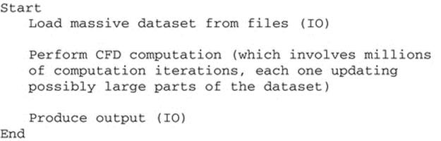
FIGURE 2.17 WeatherForecaster compute-intensive program (perform extensive CFD computation on a massive dataset).

Balanced Processes

The term “balanced” could be used to describe a process that not only uses the CPU moderately intensively but also performs IO at a moderate level. This terminology is used in the Operating Systems Workbench (see the accompanying resources). An example of this category of program could be a word processor that spends much of its time waiting for user input but that also incorporates computationally intense activities such as spell-checking and grammar checking. Such functionality may be activated automatically or on demand by the user and require short bursts of significant amounts of processing resource.

Figure 2.18 shows pseudocode for a “balanced” program the behavior of which is sometimes IO-intensive and sometimes compute-intensive. Such a process would have periods where it spends much of its time in the blocked state, but there would also be periods where it moves predominantly between the run and ready states.

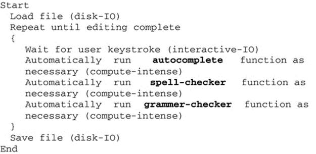
FIGURE 2.18 Word processor “balanced” program (alternates between IO-intensive behavior and bursts of high-intensity computation).

2.3.1.4 Scheduler Behavior, Components, and Mechanisms

The act of moving a process from the ready state to the running state is called “dispatching,” and this is performed by a subcomponent of the scheduler called the dispatcher. The dispatcher must ensure the appropriate preparation is carried out so that the process can operate correctly. This involves restoring the process' state (e.g., the stack and also the program counter and other operating system structures) so that the process' run-time environment (as seen by the process itself) is exactly the same as it was when the process was last running, immediately before it was preempted or blocked. This changing from the running context of one process to the running context of another is called a context switch. This is the largest component of the scheduling overhead and must be done efficiently because the CPU is not performing useful work until the process is running again. As the program counter is restored to its previous value in the process' instruction sequence, the program will continue running from the exact place it was interrupted previously. Note that this is conceptually similar to the mechanism of returning from a function (subroutine) call. The dispatcher is part of the operating system, and so it runs in what is called “privileged mode”; this means it has full access to the structures maintained by the operating system and the resources of the system. At the end-of-doing its work, the dispatcher must switch the system back into “user mode,” which means that the process that is being dispatched will only have access to the subset of resources that it needs for its operation and the rest of the system's resources (including those owned by other user-level processes) are protected from, and effectively hidden from, the process.

2.3.1.5 Additional Process States: Suspended-Blocked and Suspended-Ready

The three-state model of process behavior discussed above is a simplification of actual behavior in most systems; however, it is very useful as a basis on which to explain the main concepts of scheduling. There are a few other process states that are necessary to enable more sophisticated behavior of the scheduler. The run, ready, and blocked set of states are sufficient to manage scheduling from the angle of choosing which process should run (i.e., to manage the CPU resource), but do not provide flexibility with respect to other resources such as memory. In the three-state model, each process, once created, is held in a memory image that includes the program instructions and all of the storage required, such as the variables used to hold input and computed data. There is also additional “state” information created by the operating system in order to manage the execution of the process; this includes, for example, details of which resources and peripherals are being used and details of communication with other processes, either via pipelines as we have seen earlier or via network protocols as will be examined in Chapter 3.

Physical memory is finite and is often a bottleneck resource because it is required for every activity carried out by the computer. Each process uses memory (the actual process image has to be held in physical memory while the process is running; this image contains the actual program instructions, the data it is using held in variables, memory buffers used in network communication, and special structures such as the stack and program counter which are used to control the progress of the process). The operating system also uses considerable amounts of memory to perform its management activities (this includes special structures that keep track of each process). Inevitably, there are times when the amount of memory required to run all of the processes present exceeds the amount of physical memory available.

Secondary storage devices, such as hard disk drives, have much larger capacity than the physical memory in most systems. This is partly because of the cost of physical memory and partly because of limits in the number of physical memory locations that can be addressed by microprocessors. Due to the relatively high availability of secondary storage, operating systems are equipped with mechanisms to move (swap-out) process images from physical memory to secondary storage to make room for further processes and mechanisms to move (swap-in) process images back from the secondary storage to the physical memory. This increases the effective size of the memory beyond the amount of physical memory available. This technique is termed virtual memory and is discussed in more detail in Chapter 4.

To incorporate the concept of virtual memory into scheduling behavior, two additional process states are necessary. The suspended-blocked state is used to take a blocked-state process out of the current active set and thus to free the physical memory that the process was using. The mechanism of this is to store the entire process' memory image onto the hard disk in the form of a special file and to set the state of the process to “suspended-blocked,” which signifies that it is not immediately available to enter the ready or run states. The benefit of this approach is that physical memory resource is freed up, but there are costs involved. The act of moving the process' memory image to disk takes up time (specifically, the CPU is required to execute some code within the operating system to achieve this, and this is an IO activity itself—which slows things down) adding to the time aspect of scheduling overheads. The process must have its memory image restored (back into physical memory) before it can run again, thus adding latency to the response time of the process. In addition to regular scheduling latency, a suspended process must endure the latency of the swap to disk and also subsequently back to physical memory.

A swapped-out process can be swapped-in at any time that the operating system chooses. If the process is initially in the suspended-blocked state, it will be moved to the blocked state, as it must still wait for the IO operation that caused it to originally enter the blocked state to complete.

However, while swapped out, the IO operation may complete, and thus, the operating system will move the process to the suspended-ready state; this transition is labeled event-occurred. The suspended-ready state signifies that the process is still swapped out but that it can be moved into the ready state when it is eventually swapped-in.

The suspended-ready state can also be used to free up physical memory when there are no blocked processes to swap-out. In such case, the operating system can choose a ready-state process for swapping out to the suspended-ready state.

Figure 2.19 illustrates the five-state process model including the suspended-ready and suspended-blocked states and the additional state transitions of suspend, activate, and event-occurred.

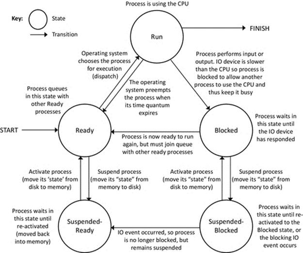
FIGURE 2.19 The extended process state transition model including suspended process states.

2.3.1.6 Goals of Scheduling Algorithms

As discussed earlier, efficiency in terms of keeping the CPU busy and thus ensuring the system performs useful work is a main goal of general-purpose scheduling. Additional goals of scheduling include the following:

• To ensure fairness to all processes
When comparing scheduling algorithms, the concept of “fairness” is usually close behind efficiency in terms of performance metrics. This is in the context of giving the various processes a “fair share” of the processing resource. However, as you shall see later when you carry out experiments with the simulations in the Operating Systems Workbench, the concept of fairness is subjective and difficult to pin down to any single universal meaning. If all processes have the same priority and importance, then it is easy to consider fairness in terms of giving the processes equal processing opportunities. However, things get much more complex when there are different priorities or when some or all processes have real-time constraints. A special case to be avoided is “starvation” in which a process never reaches the front of the ready queue because the scheduling algorithm always favors the other processes.

• To minimize scheduling overheads
Performing a context switch (the act of changing which process is running at any moment) requires that the scheduler component of the operating system temporarily runs in order to select which process will run next and to actually change the state of each of the processes. This activity takes up some processing time and thus it is undesirable to perform context switches too frequently. However, a system can be unresponsive if processes are left to run for long periods without preemption; this can contradict other goals of scheduling, such as fairness.

• To minimize process wait time
Waiting time is problematic in terms of responsiveness, and thus, a general goal of scheduling is to keep it to a minimum for all processes. Waiting time most noticeably impacts interactive processes and processes with real-time constraints, but it is also important to consider waiting time as a ratio of total run time. A process with a very short run-time requirement (in terms of actual CPU usage) will have its performance affected relatively much more than a process with a long run-time requirement, by any given amount of delay. The shortest job first, and shortest remaining job next scheduling algorithms specifically favor shorter run-time processes. This has two important effects: firstly, the shortest processes do the least waiting, and thus, the mean waiting time ratios (wait time/run time) of processes are lowered; and secondly, the mean absolute waiting times of processes are lowered because a long process waits only a short time for the short process to complete, rather than the short process waiting a long time for the long process to complete.

• To maximize throughput
Throughput is a measure of the total work done by the system. The total processing capacity of the system is limited by the capacity of the CPU, hence the importance placed on keeping the CPU busy. If the CPU is used efficiently, that is, it is kept continuously busy by the scheduler, then the long-term throughput will be maximized. Short-term throughput might be influenced by which processes are chosen to run, such that several short processes could be completed in the same time that one longer one runs for. However, as a measure of performance, throughput over the longer-term is more meaningful.

2.3.1.7 Scheduling Algorithms

First Come, First Served (FCFS)

FCFS is the simplest scheduling algorithm. There is a single rule; schedule the first process to arrive, and let it run to completion. This is a non-preemptive scheduling algorithm, which means that only a single process can run at a time, regardless of whether it uses the resources of the system effectively, and also regardless of whether there is a queue of other processes waiting, and the relative importance of those processes. Due to these limitations, the algorithm is not widely used but is included here as a baseline on which to compare other simple algorithms (see Activity P5).

Shortest Job First (SJF)

SJF is a modification of FCFS, in which the shortest job in the queue is executed next. This algorithm has the effect of reducing average waiting times, since the shortest jobs run first and the longer jobs spend less time waiting to start than if it were the other way around. This is a significant improvement, but this algorithm is also non-preemptive and thus suffers the same general weaknesses with respect to resource use efficiency as FCFS.

Round Robin (RR)

The simplest preemptive scheduling algorithm is round-robin, in which the processes are given turns at running, one after the other in a repeating sequence, and each one is preempted when it has used up its time slice. So, for example, if we have three processes {A, B, C}, then the scheduler may run them in the sequence A, B, C, A, B, C, A, and so on, until they are all finished. Figure 2.20 shows a possible process state sequence for this set of processes, assuming a single processing core system. Notice that the example shown is maximally efficient because the processor is continuously busy; there is always a process running.

FIGURE 2.20 A possible process state sequence for round-robin scheduling with three processes.

Activity P5

Using the Operating Systems Workbench to Explore Scheduling Behavior (Introductory): Comparing First-Come First-Served, Shortest Job First, and Round-Robin Scheduling

Prerequisite

Download the Operating Systems Workbench and the supporting documentation from the book's supplementary materials website. Read the document “Scheduling (Introductory) Activities and Experiments.”

Learning Outcomes

1. To gain an understanding of the first-come first-served scheduling algorithm

2. To gain an understanding of the shortest job first scheduling algorithm

3. To gain an understanding of the round-robin scheduling algorithm

4. To gain an understanding of the three-state model of process behavior

5. To reinforce the understanding of general scheduling concepts, discussed in this chapter

This activity uses the “Scheduling Algorithms—Introductory” simulation, which is found on the “Scheduling” tab of the Operating Systems Workbench. We use the same initial configuration of two CPU-intensive processes in each of the three stages below. We compare the behavior using each of three different scheduling algorithms. At the end-of-each simulation, note down the values in the statistics section at the bottom of the simulation window.

This activity is divided into three stages to provide structure.

Activity P5_CPU

Exploring first-come first-served, shortest job first, and round-robin scheduling with CPU-intensive processes

Method

Set process 1 to “CPU-intensive” and set the run time to 60 ms.

Enable process 2, set it to “CPU-intensive,” and set the run time to 30 ms.

When you are ready, press the “Free Run” button to start the simulation.

The screenshots below show the initial and final settings, respectively, when running the processes with the FCFS scheduling algorithm.

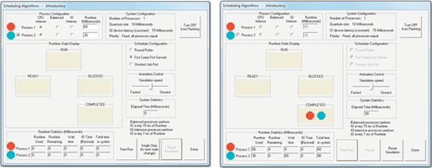
Expected Outcome

The simulation will run through the sequence of state changes for each process, until all processes have completed. You will see the run-time statistics and system statistics updating in real time as the simulation runs. These statistics enable analysis of the low-level behavior of the algorithms and their effects on the processes present.

Activity P5_balanced

Exploring first-come first-served, shortest job first, and round-robin scheduling with “balanced” processes (these are processes that perform moderate amounts of input and output but are also moderately CPU-intensive in between the IO activities)

Method

The same as for Activity P5_CPU above, except set both processes to be “balanced.”

Expected Outcome

You will see that processes get blocked when they perform IO and thus accrue time in the blocked state. You should notice a significant difference between behaviors of the three algorithms when a process becomes blocked.

Activity P5_IO

Exploring first-come first-served, shortest job first, and round-robin scheduling with IO-intensive processes (these are processes that perform IO regularly)

Method

The same as for Activity P5_CPU above, except set both processes to be “IO-intensive.”

Expected Outcome

You will see that the processes frequently perform IO and get blocked regularly and thus accrue a significant proportion of their time in the system in the blocked state. You should notice that the efficiency of the system overall is impacted if all processes are performing IO frequently, as a temporary situation can arise when there are no processes in the ready state, and thus, none can run.

Reflection

You have examined the behavior of three scheduling algorithms with a variety of differently behaved processes. Based on the run-time statistics you have collected, how do these scheduling algorithms compare to each other? Here are some specific questions to start your investigation:

1. What can be said about the fairness of the algorithms (hint: consider the waiting times for processes)?

2. What can be said about the efficiency of CPU usage (hint: consider the total time in the system for each process and the total system elapsed time)?

3. To what extent does the type of process behavior impact on the effectiveness of the scheduling algorithms? Is there always a clear winner, or do the algorithms have different strengths depending on the types of processes in the system?

Further Exploration

You can perform further experiments with the “Scheduling Algorithms—Introductory” simulation to help gain a deeper understanding. You can use the single step button to run the simulations one step at a time allowing you to work at your own pace.

The three scheduling algorithms discussed up to this point are quite limited in the context of modern general-purpose systems with a very wide variety of types of applications with very different behaviors. These scheduling algorithms lack the sophistication necessary to select processes based on contextual factors relating to dynamics of the system itself and the processes within. Some more-advanced algorithms take into account process priorities, or deadlines, or expected run time, or accumulated run time, or various other factors to improve the performance of individual processes and of the system overall. Round-robin scheduling is however ideally suited for systems in which a number of similar processes have equal importance, and as a result of its simple turn-based approach, it has the advantage of being “starvation-free,” which means that one process cannot hog the CPU at the expense of others, which can occur for extended periods, possibly indefinitely in some other schemes.

Shortest Remaining Job Next (SRJN)

SRJN is a preemptive scheduling algorithm that combines the benefits of SJF as discussed above (in which the shortest job in the queue is executed first, thus reducing the average waiting time) with the preemptive behavior of RR (which improves responsiveness by giving processes turns at using the CPU and also improves efficiency by keeping the CPU busy whenever there is a process that is ready to run). The SRJN algorithm gives processes turns at running, similar to the way in which RR does, but with the significant difference that it takes into account the amount of remaining run time (the actual amount of CPU processing time required to complete the process). The process in the ready queue with the shortest remaining run time is selected to run next. In this way, if no processes perform IO (and thus get blocked), the algorithm behaves similar to SJF because although there is preemption the previously shortest job will continue to be shortest if it gets the CPU next. However, once a process becomes blocked, another process gets an opportunity to run, thus keeping the CPU busy. It is also possible for the process ordering (in terms of remaining run time) to alter, as while one process is blocked, another may overtake it in terms of becoming the new process with the lowest remaining run time. The behavior of SRJN is explored, and compared with those of RR and SJF, in Activity P6.

Multilevel Queues

Rather than have a single ready queue, there are several, one for each different category of tasks. So, for example, there could be a queue for system processes (the highest priority), another for interactive processes and another for compute-intensive processes such as scientific computing simulations (the lowest priority). Each queue can have a different scheduling policy applied, so, for example, the compute-intensive processes could be scheduled using FIFO, while the system processes and interactive processes will need a preemptive scheme such as RR. There must also be division of the CPU resource across the different queues, as there can only be one process actually scheduled at any moment (assuming a single core). In a system that has many interactive processes, it might be appropriate to allocate perhaps 80% or more of the processing resource to the interactive processes. Where compute-intensive processes are abundant, it may be necessary to allocate more resource to this category to ensure that users get a reasonable response time while balancing this with the much shorter response times needed by the interactive processes. Note that in the example cited above, the use of FIFO scheduling would only have a localized effect on the compute-intensive process queue and would not affect the finer-grained interleaving of the RR scheduling of interactive processes. The multilevel queues algorithm is illustrated in Figure 2.21.

FIGURE 2.21 Multilevel queue scheduling.

Multilevel Feedback Queues (MLFQ)

This approach builds on the flexibility introduced with multilevel queues. Here, the processes can be moved between the queues to allow the scheduling to achieve a balance between short-term scheduling to achieve responsiveness of tasks and longer-term scheduling to ensure fairness and system efficiency.

The queues are organized in terms of priority, with the top queue having the highest priority and thus being scheduled first. Within each queue, FIFO scheduling is used. A new process enters at this level. If the process uses its entire quantum, but does not complete during that quantum, it is downgraded to the next queue level. However, if the process relinquishes control during the first quantum, it remains at the same level. Processes that perform IO and thus become blocked get promoted to the next highest queue. These rules are applied iteratively and at all priority levels such that the priority level of processes is continuously adjusted to reflect their behavior. For example, a compute-intensive process will gradually work its way down to the lowest-priority queue. However, if after a long period of computation the same process began a series of IO operations to deliver its results, or read in further data, it would climb back up some priority levels (because the IO operations cause the process to be blocked before its quantum expires).

This strategy gives priority to short tasks because they will begin at the highest priority and may complete at that level or a few levels down. IO-intensive tasks are also prioritized because they are likely to block before using their time quantum generally, thus ensuring that they are likely to remain at the higher levels of scheduling priority. Compute-intensive tasks do not fare so well in this scheme, as they will work their way down the queue levels and remain at the lowest level, where they are scheduled in RR fashion until they complete. At this level, the tasks only receive processing resource when there are no ready tasks at higher-priority levels.

The interqueue scheduling is performed strictly on a queue-priority basis, so that if there are any processes in the highest queue, they will be scheduled in a locally FIFO manner (i.e., with respect to their position in the particular queue). When the ready queue is temporarily exhausted because processes either complete, are blocked, or demoted, the next level down queue is serviced. If tasks arrive in higher-level ready queues, the scheduler moves back up to the highest populated queue and schedules tasks from there.

The multilevel feedback queue algorithm is illustrated in Figure 2.22.

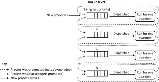
FIGURE 2.22 The MLFQ scheduling algorithm.

Figure 2.23 shows the MLFQ algorithm in operation in a system with a mix of interactive and compute-intensive processes. Initially, two processes are in the highest-priority queue (snapshot 1). P1 is a long-running interactive process so this will tend to stay at the top level. P2 however is compute-intensive and gets preempted, thus dropping to priority level 2, while a new process P3 joins the system (snapshot 2). P3 is a short-lived interactive task and thus stays at the highest-priority level, while P2 descends further (snapshot 3). P4, which is a short-lived compute-intensive process, joins (snapshot 4), while P2 descends to the lowest queue level. P4 descends one level in snapshot 5. P4 and P3 complete in snapshots 6 and 7, respectively.

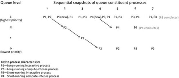
FIGURE 2.23 MLFQ example with two interactive processes and two compute-intensive processes.

Activity P6

Using the Operating Systems Workbench to Explore Scheduling Behavior (Advanced): Comparing the Shortest Job First, Round-Robin, and Shortest Remaining Job Next Scheduling Algorithms

Prerequisite

The instructions below assume that you have obtained the Operating Systems Workbench and the supporting documentation as explained in Activity P5.

Read the document “Scheduling (Advanced) Activities and Experiments.”

Learning Outcomes

1. To gain an understanding of the shortest remaining job next scheduling algorithm

2. To compare the shortest remaining job next scheduling algorithm with the shortest job first and round-robin scheduling algorithms

3. To discover the features of the Advanced Scheduling simulation of the Operating Systems Workbench, which can be used to support additional exploration

4. To further reinforce the understanding of general scheduling concepts, discussed in this chapter

This activity is divided into three sections to provide structure.

Activity P6_CPU

Comparing shortest remaining job next with shortest job first and round-robin scheduling with CPU-intensive processes.

Method

This activity uses the “Scheduling Algorithms—Advanced” simulation, which is found on the “Scheduling” tab of the Operating Systems Workbench. The advanced scheduling simulation facilitates deeper investigation into scheduling behavior. It supports an additional scheduling algorithm and up to five processes and allows configuration of the IO device latency and the scheduling quantum size:

1. We use the same initial configuration of five CPU-intensive processes and compare the behavior using each of three different scheduling algorithms. At the end-of-each simulation, note down the values in the statistics section at the bottom of the simulation window.

2. Configuration:

Set process 1 to “CPU-intensive” and set the run time to 60 ms.

Enable process 2, set it to “CPU-intensive.” and set the run time to 50 ms.

Enable process 3, set it to “CPU-intensive,” and set the run time to 40 ms.

Enable process 4, set it to “CPU-intensive,” and set the run time to 30 ms.

Enable process 5, set it to “CPU-intensive,” and set the run time to 20 ms.

Set the IO device latency to 10 ms initially (this will not have any effect when all processes are CPU-intensive), and set the quantum size to 10 ms. Set the scheduling algorithm initially to shortest job first.

3. When you are ready, press the “Free Run” button to start the simulation. Repeat the simulation with the same configuration, but using the round-robin and then shortest remaining job next scheduling algorithms. Note the results in the run-time statistics and system statistics windows. These will be used to compare the performance of the different scheduling algorithms.

The screenshots below show the initial and final settings, respectively, when running the processes with the round-robin scheduling algorithm.

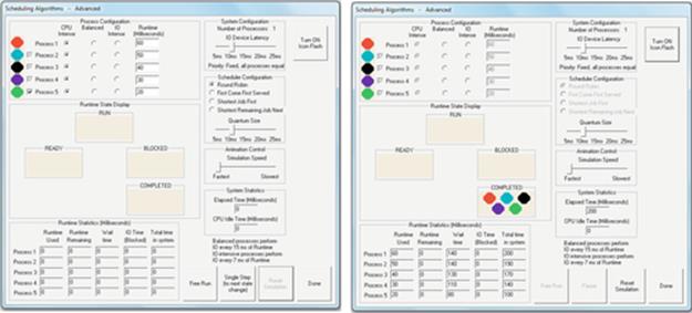
Expected Outcome

The simulation will run through the sequence of state changes for each process, until all processes have completed. You will see the run-time statistics and system statistics updating in real time as the simulation runs, as with the introductory scheduling simulation. These statistics enable analysis of the low-level behavior of the algorithms and their effects on the processes present. It is very important to pay attention to these statistics, when evaluating the relative performance of the algorithms. In the earlierActivity P5, there were only two processes so it was reasonably easy to predict the outcome of the scheduling. With five processes, the run-time system becomes quite complex, and thus, we rely on these automatically generated statistics to compare the behavior of the scheduling algorithms.

Activity P6_balanced

Comparing shortest remaining job next with shortest job first and round-robin scheduling with “balanced” processes

Method

The same as for Activity P6_CPU above, except set all processes to be “balanced.” This time, in addition to changing the scheduling algorithm, also investigate the effects of changing the IO device latency and the quantum size.

Expected Outcome

You will see that processes get blocked when they perform IO and thus accrue time in the blocked state. You should notice a significant difference between behaviors of the three algorithms when a process becomes blocked. In particular, pay attention to the wait time and the IO time, and see how these are affected by the various configuration changes.

Activity P6_IO

Comparing shortest remaining job next with shortest job first and round-robin scheduling with “IO-intensive” processes

Method

The same as for Activity P6_balanced above, except set all processes to be “IO-intensive.” Once again, be sure to investigate the effects of various configurations of IO device latency and the quantum size.

Expected Outcome

You will see that the processes frequently perform IO and get blocked regularly and thus accrue a significant proportion of their time in the system in the blocked state. You should notice that the efficiency of the system overall is impacted if all processes are performing IO frequently, as a temporary situation can arise when there are no processes in the ready state, and thus, none can run. Look at the automatically generated statistics and try to determine which scheduler is the all-round best performer (good performance being indicated by low wait times and total time in the system for individual processes and by low CPU idle time for the system).

Reflection

You have examined the behavior of three scheduling algorithms with a variety of differently behaved processes and system configurations. By having five processes, the system can exhibit significantly more complex behavior than the earlier two-process introductory simulations. This richer scenario is better in terms of finding the strengths and weaknesses of the various scheduling algorithms. Based on the run-time statistics you have collected, how do these scheduling algorithms compare to each other? Here are some specific questions to start your in vestigation:

1. What can be said about the fairness of the algorithms (hint: consider the waiting times for processes). Do processes ever get “starved,” that is, where they have to wait a long time without getting any share of the CPU?

2. What can be said about the efficiency of CPU usage (hint: consider the CPU idle time). Do situations occur where the CPU is unnecessarily idle?

3. To what extent does the type of process behavior impact on the effectiveness of the scheduling algorithms? Is there always a clear winner, or do the algorithms have different strengths depending on the types of processes in the system?

4. To what extent is the SRJN algorithm “the best of both worlds” by taking attributes of SJF and RR. Are there any negative aspects that you can detect from the experiments you have carried out?

Further Exploration

Further experimentation with the “Scheduling Algorithms—Advanced” simulation is strongly encouraged to help gain a deeper understanding. For example, try using a mixture of different process types in the same simulation. You can use the single step button to run the simulations one step at a time allowing you to work at your own pace.

2.4 Scheduling for Real-Time Systems

Real-time scheduling is the term used to describe scheduling algorithms that base their scheduling decisions primarily on the deadlines of tasks, or the periodicity of tasks, tasks being individual activities produced by processes in the system.

Examples of real-time applications include audio and video streaming, monitoring and control (e.g., fly-by-wire systems, factory automation, and robotics), as well as commercial systems such as stock trading, which are highly sensitive to delay.

Real-time processes often have a periodic behavior, in which they must service events at a given rate; for example, a video streaming application that transmits video frames at a rate of 24 frames per second must (as the description suggests) produce 24 frames of video per second. In fact, the constraint is even tighter; it is not adequate to just require 24 frames per second because that could lead to bunching and then gaps; this variation in timing is known as jitter and has a serious impact on the quality of the video stream. What is actually required is an even distribution of the frames in time, so actually, there is a requirement that the frames are spaced 1/24th of a second apart. In such a system, the scheduler needs to be aware of this requirement, so that the video streaming process gets sufficient processing time to produce the frames, at the regular intervals required.

The timing constraints of real-time tasks require careful design of the entire system. In the video example above, there are actually several behavioral constraints arising from the specified frame rate. In addition to the fact that frames must be produced at a constant rate with equal spacing, these must also be delivered across the network to the consumer, maintaining this even spacing. This is a significant challenge for real-time distributed systems. The network technology itself can cause varying delay to the video data stream (and thus introduce jitter, reducing the final quality as perceived by the user). There is also a requirement that each video frame must actually be processed before the next one arrives. So if frames are produced every 1/24th of a second, the maximum processing time available to deal with each frame (e.g., video compression actions) is thus 1/24th of a second; no longer is allowed because that would cause the frame to be delayed, and with each subsequent frame, the delay would increase further. To put this into context, I will briefly describe a system with very tight timing constraints. In the 1980s, I developed a speech recognition system that sampled and digitized the sound input at a rate of 8 kHz. The processor was a Motorola MC68010 running at 10 MHz, which was a typical operating speed at the time, but in the order of one thousand times slower than today's technology. Each sound sample had to be processed within the 125 μs intersample timeslot. The processing included looking for start-of-word, end-of-word, and detecting various characteristics of the energy signature in a word, as well as measuring the duration of silence periods. With a clock speed of 10 MHz, the processor only just had enough clock cycles to finish one sample before starting the next. After painstaking optimization, the worst-case path through my code left just 3 instruction times spare between finishing processing one sample and starting the next.

We can divide real-time systems into “hard,” “firm,” and “soft” categories. A hard real-time system is one in which a missed deadline has severe consequences (in the context of the application and its users). The most common examples of this type of systems are in control systems such as fly-by-wire systems and robotic control systems. Missing the deadline in these systems is unacceptable, and much emphasis is placed on the design and testing stages to ensure this cannot happen. Systems in the “firm” category require that deadlines are met most of the time, but occasional deadline misses can be tolerated. An example of this could be an automated stock-trading system, which attempts to execute deals at high speed to achieve the current advertised price of a stock when a specific threshold in price has been reached. For these systems, speed is essential and the design will incorporate certain assumptions of transaction response time. A soft real-time system is one where deadline misses have an impact that affects the QoS, but the system can still function and the impact is thus less serious. For example, the responsiveness of an event-driven user interface can be considered to be real time if the application involves some activity where the user needs a time-bounded response. If the user has an expectation of a particular response time, then violation of this could have an impact ranging from dissatisfaction (e.g., if results from database queries are delayed) to considerable financial loss (e.g., in an e-commerce application if an order is placed based on out-of-date information or if the order is placed but lack of responsiveness causes delay in the order being actioned). A large proportion of commercial distributed systems can be classed as soft real-time systems or will at least have some soft real-time processing requirements.

General-purpose schedulers (i.e., non-real-time schedulers) do not prioritize tasks based on their periodicity or deadlines; typically, they are not even aware of deadline as an attribute of processes or tasks generated by processes. These schedulers are however commonly found in use in nonspecialized systems, and therefore, many tasks with soft real-time characteristics (especially business applications) run on systems driven by general-purpose schedulers. There is also a challenge with respect to prioritizing tasks within business and e-commerce applications in the sense that all users consider their own tasks (such as their database queries or their file downloads) to be the most important of all and do not have a business-wide view of what is actually the most important task for the system to perform at any particular moment. Hence, in such scenarios, if users could provide deadline parameters for their tasks, it is possible that all would choose the highest-priority value offered, and of course, this is self-defeating.

2.4.1 Limitations of General-Purpose Schedulers for Real-Time Systems

Consider the situation we explored in Activity P3 in which the PeriodicOutput processes perform tasks at fixed periods. Imagine that the tasks must occur at a specific rate to ensure a particular QoS, as, for example, in processing video frames in a video streaming application. With a general-purpose scheduler, it may be possible to achieve a specific timing when there is only one active process in the system, but there is no guarantee that timing constraints (deadlines) will be preserved when there are other processes competing for the resources of the system. This is explored in Activity P7, in which three instances of the PeriodicOutput program are used to represent a pseudo real-time application in which regular interleaving of tasks is required. The activity shows how a non-real-time scheduler may be able to achieve this in the absence of compute-intensive background tasks, but when a compute-intensive task is abruptly inserted, the schedule sequence becomes unpredictable, as the compute-intensive task is favored in terms of CPU allocation (it does not block as the IO-intensive ones do).

For hard real-time systems, actually determining the deadline for tasks is usually straightforward because it relates directly to the characteristics of the task itself: the real-world events that are involved, their periodicity, and the processing that needs to be carried out as a result.

Activity P7

Examining Scheduling Behavior with Real Processes— Real-Time Considerations

Prerequisites

The instructions below assume that you have obtained the necessary supplemental resources as explained in Activity P1.

Learning Outcomes

This activity explores the nature of real-time behavior and the limitations of general-purpose schedulers in terms of ensuring deadlines are met:

1. To understand that real-time tasks have timing constraints

2. To understand that general-purpose schedulers do not cater for the timing requirements of real-time tasks

3. To understand how the behavior of real-time tasks can be affected by background workloads

Method

This activity uses the PeriodicOutput program we used in Activity P3 as a pseudo real-time program, and we also use the CPU_Hog CPU-intensive program we used in Activity P4 to create a heavy background workload:

1. Start the Task Manager as in Activity P4 and select the “Processes” tab. Sort the display in order of CPU-use intensity, highest at the top. This will provide a means of inspecting the computer's workload, so leave the Task Manager window open, to the side of the screen. Initially, the computer should be effectively “idle”—this is a term used to describe a computer with no or very little workload (typically CPU utilization will be no more than a few percent).

2. Open two command windows. In each one, navigate to the “ProcessView” subfolder of the SystemsProgramming folder.

3. In one of the command windows, run the PeriodicOutput_Starter.bat batch file. Observe the output; the A's B's, and C's produced by the first, second, and third copies of the program should be reasonably evenly interleaved as we saw in Activity P3. This observation being important, we shall use this interleaving as a pseudo real-time requirement, that is, that the processes produce output alternately. It does not really matter what the processes are actually doing, because the investigation here is concerned with how the background workload of the system can affect the behavior of the scheduling itself.

4. Once the processes running in step 3 have completed, restart them using the same batch file. This time, approximately half-way through their progress, start four copies of the CPU_Hog.exe program using the CPU_Hog_4Starter.bat batch file in the other command window. This creates a significant background workload on the computer, which the scheduler must manage.

5. Observe the effect of the CPU_Hog processes in the Task Manager window. You should also examine the effect of the sharp increase in workload on the interleaving of the output from the PeriodicOutput processes.

The screenshot below from my computer shows the effect that the CPU_Hog processes had on the interleaving of the output of the PeriodicOutput processes.

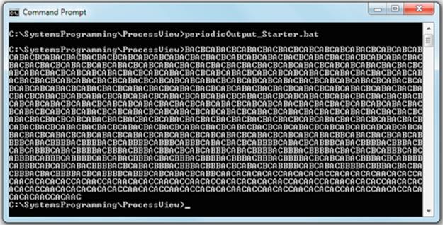
Expected Outcome

You should see something similar to my screenshot, although the actual behavior is sensitive to exactly which scheduler variant is present. In the screenshot, we can clearly see the behavior before and after the CPU_Hog background workload was started. Initially, the three copies of the PeriodicOutput process were running and their output was interleaved as we would expect. Just after half-way through this experiment, the CPU_hog processes were started in the second command window. You can see that the impact on the PeriodicOutput processes (which regularly perform IO and thus block) was that they received less regular CPU timeslots. The effect of this shows up as a disruption of the interleaving, as the three processes have to wait in the blocked state and then rejoin the ready queue, which always has at least three of the four CPU_Hog processes too, because these processes never block. This is a simple yet very important demonstration of the ways in which the performance of one process can be impacted by the behavior of the other processes that constitute the workload of the host computer. It also demonstrates how the workload intensity can change suddenly and by significant amounts and thus illustrates how difficult it can be to accurately predict process performance or system-wide behavior.

Reflection

This experiment illustrates the limitations of general-purpose schedulers with respect to process ordering and resource sharing. As the scheduler is unaware of any deadline or periodic behavior requirements of its processes, it simply shares the CPU resource based on the process state model. As most real-time tasks are also considerably IO-intensive (consider video streaming, voice and music applications, and reading sensors or making control outputs in machinery), it is likely that they will get blocked regularly, thus having to wait for events and IO hardware mechanisms, before joining the ready queue again. Therefore, these types of task are the most noticeably affected by abrupt changes in system workloads, as we have seen in this activity.

Consider a subsystem in a fly-by-wire⁵ system in which a user provides control inputs at a remote command station (e.g., the cockpit of an airplane). The commands must be auctioned within a short time frame such that they take effect on the aircraft as soon as possible after the command has been issued. The user (in this case the pilot) receives feedback through the corresponding change in behavior of the airplane. In some scenarios, there may be a need to apply a control input progressively, using the feedback as an indication of when to ease off. For such a situation, an end-to-end response time of a few tens of milliseconds might be appropriate, that is, the time between the user proving a control input, the system acting upon it, and the user receiving feedback. Thus, for a given input (which becomes a task in the system), a deadline can be determined. A deadline miss in this scenario translates into delayed response and the airplane becomes difficult or impossible to fly. There may be a marginal point at which the delay causes the airplane to respond in jerky movements as the pilot gets confusing feedback from his actions leading to alternation between overcontrol and compensation inputs. A slight increase in delay beyond this point and the airplane is totally unstable and unflyable. Figures 2.24 and 2.25 provide a simplified illustration of this scenario; T_Response is the response time of the control system once the pilot's request has been auctioned; for safe operation, this must be completed by the feedback deadline.

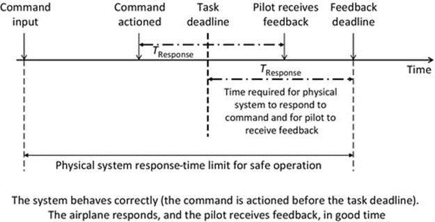
FIGURE 2.24 Simplified illustration of the importance of meeting the deadline in a hard real-time system such as a fly-by-wire vehicle.

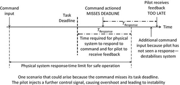
FIGURE 2.25 Simplified illustration of the importance of meeting the deadline in a hard real-time system such as a fly-by-wire vehicle.

Figures 2.24 and 2.25 provide an example of how a computer task deadline in a real-time system (in this case, a fly-by-wire aircraft control system) maps onto the boundary between safe behavior (Figure 2.24) and unsafe behavior (Figure 2.25). In such systems, it is necessary for the computer system to achieve responsiveness as close to that of systems with a direct mechanical linkage as possible. This is explained in terms of the control systems of two very different aircraft. The Tiger Moth is an iconic biplane developed in the 1930s. Its handling was found to be suitable for use as a pilot trainer and was actually used to train Spitfire pilots during the Second World War. The Moth has direct cable linkages from its central joystick to the ailerons on the wings. You push the stick forward and the plane will dive, pull it back and it climbs, and push it left or right and it performs a banked turn to the left or right, respectively. The pilot receives instant feedback from her actions through the movement of the plane. If, for example, the pilot feels the plane is climbing too steeply, she will ease off on the stick, moving it towards the central position, and the climb will level off. The Moth is very responsive and easy to fly and the control system is very simple—there is no latency added by the control system itself. The pilot's actions in moving the stick translate directly and instantly in the equivalent movement of the ailerons. Now, compare the Moth with modern airliners, which are fly-by-wire with some very sophisticated control systems and in which some of the control surfaces are extremely heavy and large. The pilot demands a system that is as responsive as that of the Moth (having been privileged to have flown a Tiger Moth, I can confirm that the control inputs do indeed have immediate effect and the plane is highly responsive as a result). The modern plane has a vast array of safety systems, sensors, and actuators; to manage these systems, a great many computational processes can be active on its onboard computers at any moment. This is a very good example of a hard real-time system in which various tasks have different deadlines and priorities. There is a need to deal with routine sensor signals on a periodic basis, as well as unpredictable (asynchronous) events such as alarm signals indicating detected faults while ensuring that the control signals to move control surfaces do not miss their deadlines. The various computation and control activities must each be carried out within strict deadlines and the priorities of different tasks may change depending on the flight context, such as whether the plane is taking off, in smooth flight, in turbulent conditions, or landing.

As Figure 2.25 shows, a delay to a control action could lead to additional inputs from the pilot, which leads to overcompensation and ultimately destabilization of the aircraft.

A process that deals with inputs from a joystick could be an example of a periodic process, generating periodic tasks. Instead of detecting joystick movements and reacting to each, a more likely approach is to read the joystick position at a suitably high rate and communicate the value to the control surfaces regardless of whether the stick has been moved or not. In this way, the control surfaces always follow the stick's position with a certain lag, which is the total of the time to read the sensor, process the data to compute the control surface position, transmit the command to the actuator (such as on the wing), and actually move the control surface. The total latency must be small enough that the pilot gets a natural response from the plane; ideally, there should be the illusion of direct cable connection to the stick, pulling the ailerons. In addition to low latency, the actual latency must be consistent so that the pilot gets a predictable and consistent response from the plane; the scheduler must ensure this even when dealing with other urgent actions.

For illustration, consider that the sampling rate could be perhaps 100 Hz (i.e., sample the position of the control stick 100 times a second). The total latency allowed once sampling has occurred might be perhaps 50 ms. This means that the total time delay, between the stick being moved and the aircraft's control surface following it, would be 50 ms plus up to 10 ms due to the sampling interval (i.e., if the stick was moved immediately after sampling, then a further 10 ms would elapse before the new movement would be detected).

Many real-time monitoring and/or control systems include periodic tasks where a sensing activity and a subsequent control activation are performed with a regular time period (as in the aircraft joystick example discussed above). Often, there will be multiple streams of periodic tasks, generated by different processes. For example, playing a movie may involve two different streams of tasks, one for the video frames and one for the sound. In this case, the timing relationships not only within the streams but also between the streams must be maintained (so that the sound and vision remain synchronized). Scheduling for such systems has some specific requirements, including the need to maintain the interval between the execution of tasks in a given stream and the need to schedule all tasks from all streams within their time constraints. The CPU processing capacity is a limiting factor in the rate at which tasks can be performed. The utilization of the CPU (for a given stream of tasks) depends on a combination of the period between the tasks and the computation time needed for each task instance.

The formulas to compute CPU utilization for periodic tasks are shown in Figure 2.26. The left-hand formula is for a single periodic task stream (continuous stream of tasks), while the right-hand formula is for a set of n periodic task streams. C is the computation time per task instance (within a stream), P is the intertask period, and U is the resulting CPU utilization as a fraction between 0 and 1. For the right-hand formula, n is the number of periodic task streams in the concurrent set, and i signifies a specific periodic task stream in the set {1 … n}.

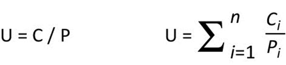
FIGURE 2.26 CPU utilization formulas for periodic tasks.

The lower the utilization U, the more likely that all tasks can be scheduled correctly. If U exceeds 1.0, then the system is overloaded and some tasks will definitely be delayed. Even at values of U that are below 1.0 where there are multiple streams of tasks, it is possible that some specific task instances will be delayed because of the interleaving requirements of the multiple streams. Table 2.1 illustrates the way the utilization formulas work with some example configurations for a single periodic task stream P₁ {P₁T₁, P₁T₂ … P₁T_n} and for two periodic task streams P₁ {P₁T₁, P₁T₂ … P₁T_n} and P₂ {P₂T₁, P₂T₂ … P₂T_n}.

Table 2.1

CPU Utilization Examples

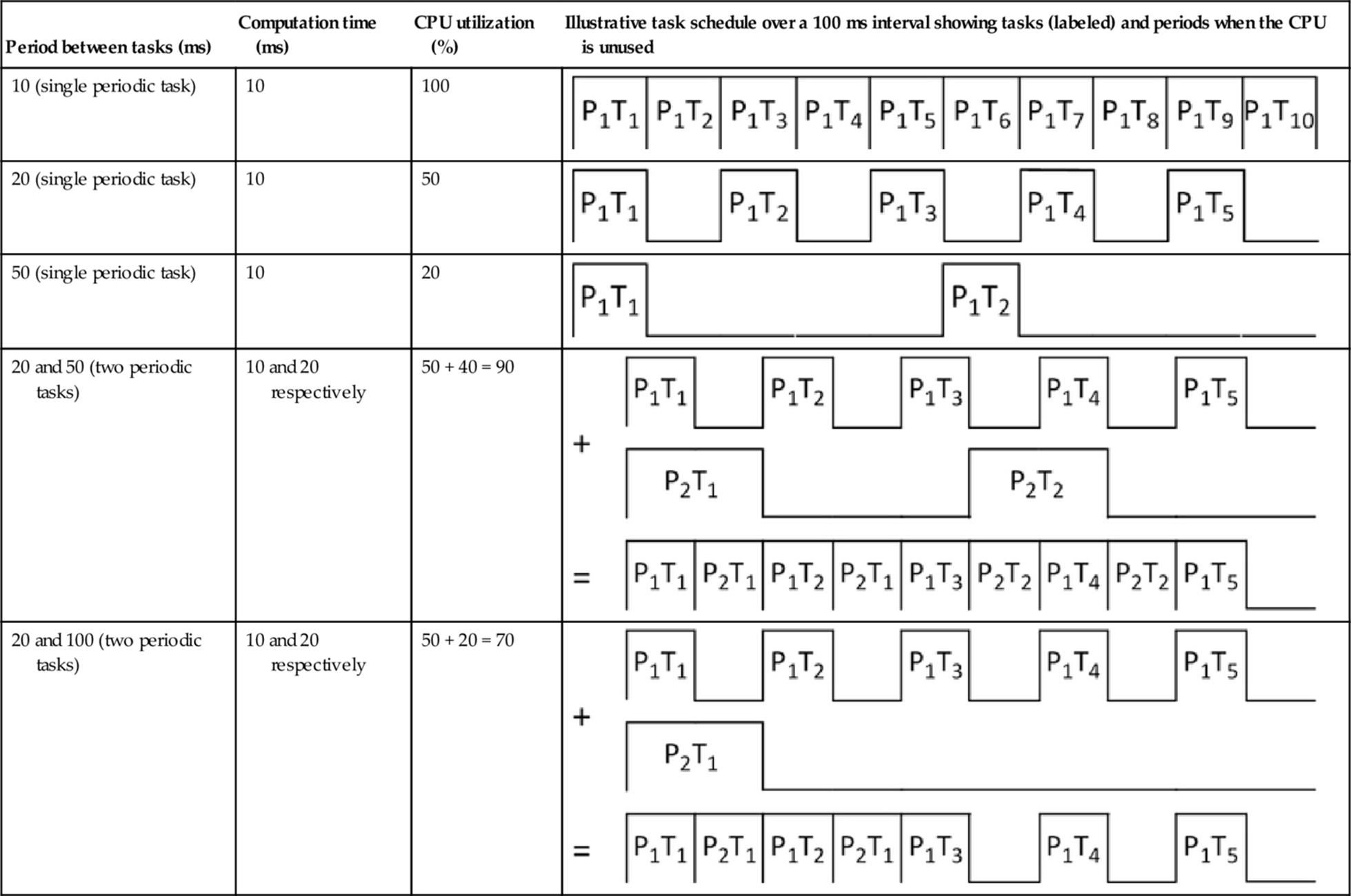
2.4.1.1 The Deadline Scheduling Algorithm

Deadline scheduling orders tasks by their deadlines, the task with the earliest deadline being run first. This has the effect that the task's deadline is its priority. The deadline scheduling approach does not pay attention to the interval between tasks that are generated periodically by a process. Therefore, while deadline scheduling is very good at meeting deadlines (because this is its only criterion when choosing tasks), it is not so good at preserving a regular spacing of tasks, which is necessary in, for example, audiovisual applications where the interframe spacing is an aspect of QoS or, for example, in a highly precise monitoring or control application where the sampling and/or control inputs must be evenly spaced in the time dimension.

2.4.1.2 The Rate Monotonic Scheduling Algorithm

Rate monotonic scheduling assigns a priority value to each process, based on the period of the tasks it generates, the process with the shortest intertask period having the highest priority. This emphasis on the period, rather than the deadline, leads to distinctly different behaviors from that of deadline scheduling under some circumstances. This approach is far better suited for systems that have repetitive streams of tasks generated by processes at regular intervals, where the interval itself is an important aspect of the system's performance. However, in emphasizing the value of preserving the interval, this algorithm is not as good as deadline scheduling at meeting deadlines in some situations.

Activity P8 investigates the behavior of the deadline and rate monotonic real-time scheduling algorithms using a variety of different real-time task mixes.

Activity P8

Using the Operating Systems Workbench to Explore Scheduling for Real-Time Systems (Introductory): Comparing Deadline and Rate Monotonic Scheduling Algorithms

Prerequisite

The instructions below assume that you have obtained the Operating Systems Workbench and the supporting documentation as explained in Activity P5.

Read the document “Real-Time Scheduling (Introductory) Activities.”

Learning Outcomes

1. To gain an understanding of the nature of real-time processes, especially with respect to deadlines

2. To appreciate the differences between real-time schedulers and general-purpose schedulers

3. To gain an understanding of the rate monotonic scheduling algorithm

4. To gain an understanding of the deadline scheduling algorithm

Method

This activity uses the “Real-Time Scheduling—Introductory” simulation, which is found on the “Scheduling” tab of the Operating Systems Workbench. The simulation supports up to two real-time processes with periodic tasks. For each process, the intertask period and the CPU-time requirement per task can be configured. Two real-time scheduling algorithms are provided: deadline and rate monotonic. The simulation calculates the CPU utilization for the schedule, based on the configuration of the processes. A real-time moving display is provided, showing the current time (the vertical black line), the task's approaching deadlines (the vertical arrows to the right), and a recent history of the scheduled tasks (to the left):

1. Configuration. For process 1, set the period to 33 ms and computation time to 16 ms. Enable process 2 and set the period to 20 ms and computation time to 10 ms. Select the deadline scheduling algorithm initially.

2. Notice the CPU utilization calculation that is shown. Look at the formula that has been used (this is dynamically updated depending on how many processes are active). Can you see how this formula works? See discussion earlier in the text.

3. When you are ready, press the “Free Run” button to start the simulation; let it run for some time, long enough to appreciate the scheduling behavior. Repeat the simulation with the same configuration, but using the rate monotonic scheduling algorithm instead. Note the results in the run-time statistics and system statistics windows. These will be used to compare the performance of the different scheduling algorithms.

4. Repeat the experiment (for both schedulers), but this time, use the following process configurations:

• for process 1, period = 30 ms, computation time = 7 ms,

• for process 2, period = 15 ms, computation time = 10 ms.

What differences do you notice, in terms of the CPU utilization, the processes' task timing, and the CPU idle time (look at the third horizontal display line with the green bars representing CPU idle time)?

5. Repeat the experiment, for both schedulers again, now using the following process configurations:

• for process 1, period = 30 ms, computation time = 16 ms,

• for process 2, period = 20 ms, computation time = 10 ms.

What happens to the CPU utilization, the processes' task timing, and the CPU idle time under these conditions? Note that red bars indicate the task is overdue.

The screenshot below provides a snapshot of the deadline simulation soon after it was started. The two processes have completed one task each and these tasks have both met their deadlines (the tasks ended before the vertical arrows that signify their deadlines). The second task of process 2 has begun and has had 4 ms of CPU time (see run-time statistics), of the 10 ms in total that this task needs (see the process configuration).

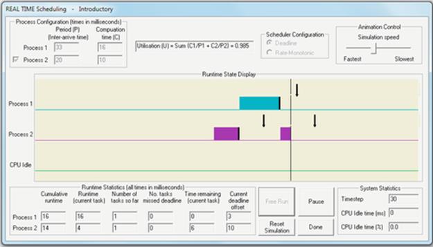
Expected Outcome

The simulations run continuously until stopped by pressing the pause or done buttons. This is because the types of process being simulated have periodic behavior in which tasks, with their own short-term deadlines, are created periodically by each process. As the tasks can be run back to back, a solid black bar marks the last time step of each task for visual clarity. You will see the run-time statistics and system statistics updating in real time as the simulation runs, as with the general-purpose scheduling simulations. These statistics facilitate analysis of the low-level behavior of the algorithms and their effects on the processes present. It is very important to pay attention to these statistics, when evaluating the relative performance of the algorithms. With real-time scheduling, the main goals are to avoid deadline misses and to maintain regular periodic task timing. Therefore, the number of tasks that miss their deadlines is generally the most important statistic to watch.

Reflection

You have examined the behavior of two real-time scheduling algorithms with a variety of process configurations. Based on the run-time statistics you have collected, you should be able to compare their behavior. Here are some questions to guide you:

1. What are the main differences in terms of the way the two algorithms perform scheduling?

2. Which is best at avoiding deadline misses?

3. Which algorithm seems to provide a more regular schedule (i.e., with regular periods between tasks)?

4. Does a CPU utilization level less than 1.0 ensure that no deadlines are ever missed?

Notice that as soon as a process' deadline expires, the scheduler calculates the next deadline for the same process; this is used as the basis for the scheduler's choice of which process to run at each time step. This awareness of deadlines is a major difference between the real-time schedulers and the general-purpose schedulers.

Make sure you appreciate how the CPU utilization calculation works. You can perform additional experiments with different process configurations to help clarify this, as necessary.

Further Exploration

Carry out additional experiments with the “Real-Time Scheduling—Introductory” simulation using a variety of different process configurations to gain a deeper understanding. In particular, look for evidence of the different task prioritization approaches of the two scheduling algorithms in the patterns of the task schedules produced.

You may want to use the single step button to run the simulations one step at a time allowing you to work at your own pace.

Introducing Variable, Bursty Workloads

In any open system, the background workload can be variable. This workload can affect the scheduler's effectiveness especially if the CPU utilization is high and all of the tasks present have real-time constraints. It is also important to realize that from the point of view of any specific process p, all other processes constitute the background workload with which it competes for resources, and thus from the point of view of those other processes, p itself is part of the background workload.

Activity P9 provides an opportunity to investigate the impact of variable workloads on real-time schedules. The advanced version of the Operating Systems Workbench real-time scheduling simulation supports three processes. In part 1 of the activity, we investigate scheduling with three periodic real-time processes. In part 2 of this activity, we use one of the processes to take the role of a bursty background workload (but whose tasks have real-time constraints), which impacts on the scheduler's ability to correctly schedule a pair of periodic real-time processes. The simulation supports configuration of a start-time offset for each process. In the second part of this experiment, we set this for the third process such that it begins in the middle of an established schedule of a pair of periodic processes. This process is configured to generate only a single task, but this has its own deadline and thus the scheduler must try to incorporate the new task into the existing schedule.

Activity P9

Using the Operating Systems Workbench to Explore Scheduling for Real-Time Systems (Advanced): Comparing Deadline and Rate Monotonic Scheduling Algorithms

Prerequisites

The instructions below assume that you have obtained the Operating Systems Workbench and the supporting documentation as explained in Activity P5.

You should have carried out Activity P8 prior to this one.

Read the document “Real-Time Scheduling (Advanced) Activities.”

Learning Outcomes

1. To gain a more detailed understanding of the nature of real-time scheduling, especially with respect to sensitivity to background workloads

2. To enhance understanding of the rate monotonic scheduling algorithm

3. To enhance understanding of the deadline scheduling algorithm

Method

This activity uses the “Real-Time Scheduling—Advanced” simulation, which is found on the “Scheduling” tab of the Operating Systems Workbench. The simulation supports up to three real-time processes with periodic tasks. For each process, the intertask period, the CPU-time requirement per task, the number of tasks, and the first task start offset can be configured, enabling simulation of a very wide range of circumstances. As with the “Introductory” simulation, two real-time scheduling algorithms are provided: deadline and rate monotonic. The simulation calculates the CPU utilization for the schedule, based on the configuration of the processes. A real-time moving display is provided, showing the current time (the vertical black line), the task's approaching deadlines (the vertical arrows to the right), and a recent history of the scheduled tasks (to the left).

Part 1. Scheduling with Three Processes

1. Configure the processes as follows:
For process 1, set the period, computation time, first instance start offset, and number of tasks to {35, 16, 0, − 1}, respectively (the − 1 means an infinite number of tasks, i.e., the process runs endlessly). Enable process 2, and similarly configure with {20, 10, 0, − 1}. Enable process 3, and configure with {25, 2, 0, − 1}. Select the deadline scheduling algorithm initially.

2. Run the simulation for some time, long enough to appreciate the scheduling behavior. Repeat the simulation with the same configuration, but using the rate monotonic scheduling algorithm instead. Note the results in the run-time statistics and system statistics windows. These will be used to compare the performance of the different scheduling algorithms.

3. What is the fundamental problem with this mix of processes? Examine the behavior until you can clearly see why this schedule will always lead to deadline misses.

4. Increase the period for task 2 until the schedule runs without deadline misses. You may need to try a few different values until you reach and acceptable configuration.

Part 2. Scheduling with a “Bursty” Background Workload

1. Processes 1 and 2 will constitute a regular real-time workload. Process 3 will represent a bursty workload, which starts abruptly, runs for a short time (causing a disturbance to the real-time scheduling), and then stops. Configure the processes as follows:
For process 1, set the period, computation time, first instance start offset, and number of tasks to {35, 16, 0, − 1}, respectively. Enable process 2, and similarly configure with {20, 10, 0, − 1}. Enable process 3, and configure with {25, 8, 100, 1}, which means that it will generate one task only, with a processing requirement of 8 ms and with a deadline of 25 ms, and will do this after a 100 ms delay. Select the deadline scheduling algorithm initially.

2. Run the simulation. Note that initially, the scheduler deals with the workload adequately. The additional task then starts and disturbs the scheduling, causing some deadline misses, and then the system settles down again once the third process has completed.

3. Repeat the experiment with the same configuration: except for process 3, which now has {50, 8, 100, 1}.

Observe the behavior—the third process has the same processing requirement as it did in the previous experiment, but this time, the processing is able to be spread over a longer time frame, which means a better opportunity for the scheduler to use any idle CPU time that may occur. Is the overall result any different this time?

The screenshot below provides a snapshot of the deadline simulation in part 1, with three processes. The CPU utilization has been calculated to be 1.037, which implies that it is not possible to meet all deadlines. We can see that one of the tasks of process 1 has missed its deadline very slightly (red bars signify an overdue task), followed by a more significant overshoot of a task of process 2.

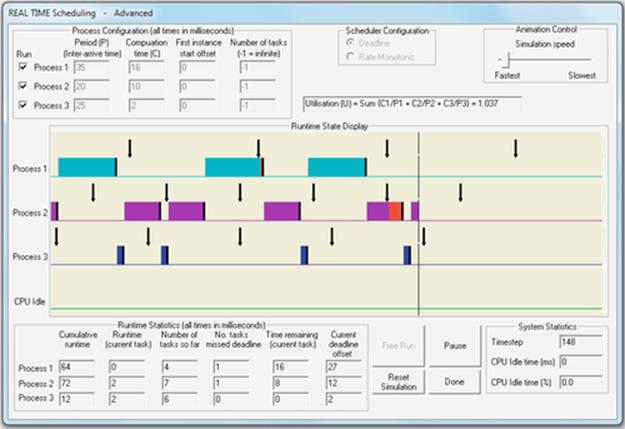
Expected Outcome

This activity has illustrated the added complexity of scheduling three real-time processes with periodic tasks and also the situation that occurs when a finely balanced two-process schedule is disturbed by the introduction of an additional process.

Reflection

As with general-purpose scheduling, CPU utilization is a main concern of real-time scheduling. In the former, an inefficient algorithm or increase in workload will have the effect of a degradation of performance generally, as tasks will take longer to execute; however, since there is no real-time constraint, it does not directly translate into a disaster. In the real-time systems, however, an inefficient algorithm or an overloaded system will lead to deadline misses. The seriousness of this will depend on the type of system. In an automated production line, it could disrupt the necessary synchrony with which the various robots operate. In automated stock trading or e-commerce, it could mean missing out on the best price in a deal. In a fly-by-wire car or aircraft, the delay of control signals reaching the control surfaces could destabilize the vehicle and lead to a crash!

We investigated the impact that background workload and fluctuations in workload can have on time-sensitive tasks. Even with real-time schedulers, a bursty background workload in which system load increases suddenly can impact the scheduling and cause deadline misses. This is an interesting challenge. The additional task could be very unlikely to occur but a very high-priority event such as closing a particular valve in an automated chemical production facility in response to an out-of-range sensor reading. The design of real-time systems thus has to consider all possible timing scenarios, including the most unlikely events, to ensure that the systems can always meet the deadlines of all tasks.

Further Exploration

Carry out additional experiments with the “Real-Time Scheduling—Advanced” simulation using a variety of different process configurations to gain a deeper understanding.

2.5 Specific Scheduling Algorithms and Variants, Used in Modern Operating Systems

Almost all popular operating systems used in general-purpose computing systems implement variants of MLFQ because of the flexibility it affords when scheduling tasks of different types. Windows NT-based operating systems use MLFQ with 32 priority levels. Priority levels 0-15 are for non-real-time processes and levels 16-31 are for processes with soft real-time scheduling requirements. Linux has used a variety of scheduling algorithms, which include a MLFQ scheduler with a range of priority levels from 0 to 140, of which levels in the range 0-99 were reserved for real-time tasks. In addition to reserving the higher-priority queue levels for real-time tasks, they are also given considerably larger quantum sizes (approximately 200 ms), while the non-real-time tasks get quanta of approximately 10 ms. AIX (a version of Unix) has supported a variety of scheduling algorithms over its various versions, including FIFO and RR. The Mac OS operating system family have used a number of different scheduling algorithms, based on preemptive kernel-level threading. OS X uses MLFQ with four priority levels (normal (lowest priority), system high priority, kernel mode only, and real-time (highest priority)).

2.6 Interprocess Communication

Communication between processes in distributed systems is necessary for a wide variety of reasons. Applications may comprise large numbers of different processes, spread across various physical computers. Some communication will be local, between processes on the same computer, and some will be between processes on different computers, perhaps with different processor architectures and/or different operating systems.

Earlier in this chapter, the pipeline was introduced as a means of communication between processes by mapping the output stream of one onto the input stream of another. This can be very useful to construct logic pipes where data flow through a number of processes, being manipulated at each step, as in the Adder | Doubler example used. However, this form of IPC operates in one direction only and the processes are directly coupled by the pipe, that is, they operate as a synchronous unit, and the second process waits on the output of the first. Another significant limitation of the pipe mechanism is that it is mediated by the process-local operating system, and thus, by implication, both processes must be located on the same physical computer.

2.6.1 Introduction to Sockets

The pipeline is only one of several IPC mechanisms available; sockets are another very important mechanism. Here, we introduce sockets in the context of IPC between local processes. The use of sockets in networking is explored in depth in Chapter 3. However, there are a few important characteristics of sockets that are mentioned briefly at this point so that their importance is recognized as you work through this section. Firstly, sockets have become a standard IPC concept that is implemented on just about every processing platform (both in terms of hardware and in terms of the operating systems that sit on the hardware platforms). Thus, the socket is an ideal basis for IPC in heterogeneous environments as it provides a means of interconnectivity between the different systems and also enhances the portability of applications. Secondly, sockets are supported by just about every programming language; this enables the components of a distributed application to be developed in different languages as appropriate for the functionality of the component. For example, in a client-server application, you might choose C++ for the back-end server processing but favor C# for the client-side graphical user-interface aspects. Finally, sockets operate at the transport layer of the seven-layer network model, and thus, socket-based IPC can be implemented using either of the TCP or UDP communication protocols.

Sockets allow communication though a dedicated channel rather than reusing the input/output streams. We are effectively creating new streams to perform the communication, facilitated by the sockets library.

The socket is a virtual resource (i.e., it is a structure within memory), which serves as an end point for communication between a pair of processes. Each socket is a resource that is associated with a specific process.

Each process can use as many sockets as necessary to permit communication with other processes. Sockets are very flexible in terms of the modes of communication they support. Sockets can be used in unicast or broadcast communication, and the processes involved can be on the same computer, or on different computers.

To set up communication, each process must first create a socket. The socket() system call is used to do this. The operating system actually creates the socket and returns the socket ID to the process, so that it can refer to the appropriate socket when sending and receiving messages. The sockets can be associated together to provide a virtual connection or can be used for discrete send and receive operations, depending on the parameters provided when the socket is created. The mechanism of using sockets to achieve IPC between processes is illustrated in Figure 2.27.

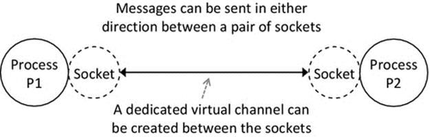
FIGURE 2.27 Sockets are end points for communication between a pair of processes.

The usage of the socket library primitives is illustrated by means of annotated code segments from the IPC_socket_Sender and IPC_socket_Receiver programs that are used in the Activity P10, which follows. In this particular scenario, the two processes are on the same computer, and unicast communication in one direction only is implemented.

Figure 2.28 presents key-code segments from the IPC_socket_Sender program. Variables are created to hold a reference to the socket and the socket address (the combination of the IP address and port number) of the recipient process; a special SOCKADDR_IN structure is used for this purpose. The socket is created inside the CreateSocket method, using the socket primitive. The send address structure is then filled out with the IP address and port number that will identify the recipient process. The user's message (preplaced in a string in code not shown here) is then sent, using the sendto primitive, which uses the previously created socket and address structure.

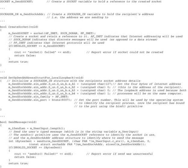
FIGURE 2.28 Annotated C++ code segments of the IPC_socket_Sender program.

Figure 2.29 presents key-code segments from the IPC_socket_Receiver program. As with the sender program, variables are created to hold a reference to the socket and the socket address (a SOCKADDR_IN structure is used again, but this time, the local address is used, i.e., it is the address on which to receive; it is interpreted as receive messages, which are sent to this address). The socket is created inside the CreateSocket method, using the socket primitive. The local address structure is then filled out with the recipients own address details. The bind primitive is used to make an association between the process and the chosen port number. This informs the operating system that any messages addressed to the specified port number should be delivered to this specific process. The recvfrom primitive is then used to retrieve a message (if one has already arrived in the receive buffer), or otherwise, the process will be blocked by the scheduler because it must wait for a message to arrive (which is an IO operation).

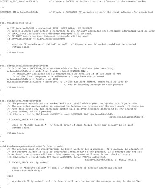
FIGURE 2.29 Annotated C++ code segments of the IPC_socket_Receiver program.

Activity P10 provides an illustration of socket-based communication between processes, using the two programs discussed above.

The sockets concepts introduced in this section and Activity P10 are very important learning outcomes at the level of the book itself and have been introduced here to link them with other aspects of the process view of systems. However, sockets are revisited and dealt with in greater depth in Chapter 3.

Activity P10

Introduction to Socket-Based Interprocess Communication (IPC)

Prerequisites

The instructions below assume that you have obtained the necessary supplemental resources as explained in Activity P1.

Learning Outcomes

This activity introduces sockets as a means of interprocess communication.

1. To understand the concept of a socket as a communication end point

2. To understand that communication can be achieved between a pair of sockets, using the sendto and recvfrom primitives

3. To understand how the local loopback special IP address can be used to identify the local computer (without having to know its actual unique IP address)

4. To understand how a port number is associated with a particular process, so that a message can be sent to that specific process when there are many processes at the same IP address

Method

This activity uses the IPC_socket_Sender and IPC_socket_Receiver programs to provide an introduction to socket-based IPC:

1. Examine the source code for the IPC_socket_Sender.cpp program. In particular, look at the way the socket primitives are used; in this program, the socket() primitive is used to create a socket, and then, the sendto() primitive is used to send a message from the created socket to another socket in another process. Also examine the socket address structure, which is configured with the IP address of the computer where the destination process is located, and the port number, which identifies the specific process (of the possibly many) on that computer. Notice that in this case, the process is located on the local computer, so the 127.0.0.1 loopback address is used and that the specific port that identifies the destination process is 8007.

2. Examine the source code for the IPC_socket_Receiver.cpp program. Look at the way the socket primitives are used, noticing some similarities with the sender program, especially the fact that a socket is created and an address structure is configured. However, there are also three important differences. Firstly, notice that the same port number is used, but this time, the bind() primitive is used—this makes an association between the receiver process and the specified port number, so that the operating system knows where to deliver the message. Secondly, the IP address used is different, in this case INADDR_ANY—this means that a message will be received by this process not only if it is sent to any address of the computer, so, for example, the special loopback address, which the sender program uses, will suffice, but also if the computer's unique IP address were used (see Chapter 3 for details), then the process would still receive the message. Thirdly, notice that recvfrom() is used to receive the message that has been sent with the sendto() primitive in the other program.

3. Open two command windows. In each one, navigate to the “ProcessView” subfolder of the SystemsProgramming folder.

4. In one of the command windows, run the IPC_socket_Receiver.exe program. This program waits for a message to be sent to it. When a message arrives, it will display it. The program should display “Waiting for message…”.

5. In the other command window, run the IPC_socket_Sender.exe program. This program waits for the user to type a message, which it then sends to the other program, via the socket-based IPC. The program should initially display “Type a message to send…”.

6. Position the two windows so that you can see both at the same time. Type a message in the IPC_socket_Sender program and press the Enter key. The message will be sent and should be displayed by the IPC_socket_Receiver program.

The screenshots below show what you should see.

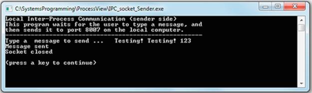
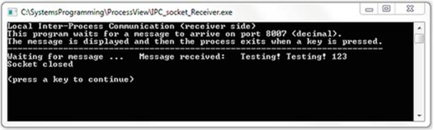
Expected Outcome

The IPC_socket_Receiver process waits for the message to arrive and then displays it, as in the example shown above. Experiment with this a few times—you are actually sending a message from one process to another, using the sockets library as the mechanism for sending and receiving the message and using the operating system as an intermediary to pass the message.

Reflection

It is important to realize that this communication between processes represents your first step towards developing distributed applications and systems. Sockets are a flexible form of IPC. With sockets, the communication can be bidirectional, the processes can be on different computers, and we can also send a broadcast message to many receivers.

Study the source code for both the sender and receiver programs and make sure that you can reconcile the logic of the two programs with the run-time behavior exhibited, especially in terms of the communication interaction that occurs between the two independent processes.

Consider the opportunities that IPC between processes on different computers opens up for you. Perhaps your interest is in e-commerce or other distributed business applications, in multiplayer games development, or in remote access to computational resources. Think about how communication between processes fits in as a major building block in all of these distributed applications.

2.7 Threads: An Introduction

2.7.1 General Concepts

A program that has a single list of instructions that run one at a time in the order that the logic of the program dictates can be said to be single-threaded (the program is said to have a single “thread of control”). In contrast, a multithreaded process has two or more threads of control. These threads can all be active at the same time and may operate asynchronously with respect to the other threads (i.e., once started, each thread gets on with its own work until it completes—it does not have to synchronize its activity with the other threads). Alternatively, their behavior may be synchronized; typically, this may involve one thread passing control (yielding) to another thread or one thread pausing until another has completed, depending on the program logic requirements and the actual threading mechanism used.

The thread that initially runs, and creates the other threads, is called the main thread of execution. The other threads are referred to as worker threads. The threads within a process share the process' resources such as memory, open files, and possibly network connections. Once started, these may need to synchronize in order to pass data from one to another or to ensure that accesses to the shared resources are performed in such a way as to prevent inconsistency; for example, if two threads were to update a shared variable independently, it is possible that one overwrites the output of the other. Access to shared resources must therefore be regulated, typically via a synchronization mechanism. Threads in some systems can be blocked (independently of the other threads) by the operating system, which improves responsiveness of the process itself. These characteristics of threads represent significant advantages over their coarser process counterparts, depending on the threading implementation and thread scheduling technique.

One advantage common to all threading schemes is that interthread communication can be achieved using shared memory within the process' address space. This means that the threads communicate by reading and writing to shared variables that they both have direct access to. This requires synchronized access to ensure consistency of the shared data but is very fast because the communication is performed at memory access speed and no context switch is needed to invoke external mechanisms, as with IPC at process level.

2.7.2 Thread Implementations

There are two distinct categories of thread mechanisms: those where the threading is visible to and supported by the operating system scheduler (and are referred to as kernel-level threading) and those that are built in user-space libraries and exist only at the process level (which are referred to as user-level threading).

Kernel-level scheduling is generally the better approach, since each thread is individually scheduled and thus a process comprising multiple threads does not get blocked when a single of its threads performs IO; only the specific thread is blocked, allowing the other threads to continue, and thus, the process can remain responsive and also can get more work done in a given span of time than if it were single-threaded. Kernel-level multithreading also offers improved performance if the threads are scheduled onto different processors or cores within the system, effectively allowing the process to use more resources than the single-threaded equivalent could.

User-level threading is useful where the kernel does not support threading directly. The scheduling of threads must be performed within the process itself. When the process is running (as viewed by the operating system), any one of its internal threads can actually be running. Threads can be preempted using programmable timer mechanisms or can hand over control to other threads when appropriate (this is referred to as yielding).

The operating system schedules the user-level threads collectively—as far as it is concerned, they are a single entity (the process), and it is not aware of the different threads. This impacts on performance in two main ways: Firstly, if one of the threads performs IO, the entire process will be blocked; and secondly, the threads cannot be spread across multiple processor cores to take full advantage of the hardware resources that are available (as kernel-level threads can).

The two approaches are compared in Figure 2.30.

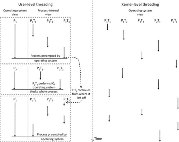
FIGURE 2.30 Comparison of user-level threading and kernel-level threading.

Figure 2.30 shows the different thread-run sequences that arise when the same pair of multithreaded processes are scheduled by user-level and kernel-level threading mechanisms, respectively. Process P₁ comprises three threads: P₁ = {P₁T₁, P₁T₂, P₁T₃}; process P₂comprises two threads: P₂ = {P₂T₁, P₂T₂}. As can be seen on the left-hand side of the figure, the internal threading of the processes in the user-level threading mechanism is invisible to the operating system, and thus, when one of the threads within a process performs IO, the entire process is blocked. In contrast, in the kernel-level threading scheme, the scheduler can run any thread in the ready queue regardless of which process it belongs to (although the selection may be influenced by other factors not discussed here such as process priority). A thread moves through the process states (run, ready, and blocked) independently of its siblings.

2.7.3 Thread Scheduling Approaches

There are two ways in which operating systems perform thread scheduling:

1. The operating system gives a thread a quantum and preempts the thread when the quantum has expired. This is termed preemptive multitasking and is similar to preemptive process scheduling.

2. Threads are started by the operating system and relinquish control when they need to stop processing, for example, when they have completed a task or must wait to synchronize with another thread. This is termed cooperative multithreading.

Preemptive multitasking allows the operating system to determine when context switches (i.e., handing control to a different thread) occur, which can be better for overall system fairness. However, cooperative multithreading allows the individual threads to hand over control at appropriate points within their processing and can therefore be more efficient with respect to the performance of individual processes, whereas operating system-driven preemption can occur at any time irrespective of thread-internal state. Cooperative multithreading requires careful logic design and can be problematic in terms of performance and efficiency if a thread does not relinquish control appropriately; it may temporarily starve other threads of processing resource, or it may hold onto the CPU while waiting for some resource to become available.

Regardless of which of these scheduling approaches are used by the operating system, it is the operating system that chooses the next thread to run, from the set that are available, that is, ready.

2.7.4 Synchronous (Sequential) Versus Asynchronous (Concurrent) Thread Operation

The thread scheduling approaches discussed above apply at the operating system level and relate to the way in which threads are actually scheduled by the system. Any thread that is able to run can be selected to run next; the developer of the program does not control this aspect.

However, depending on the actual function and logic of applications, there are situations when the developer needs to influence the thread-run ordering as part of the program logic, that is, restricting the set of threads that can be executed at a particular moment by the operating system, based on program logic-specific criteria. One common example is requiring that one particular thread pauses until another specific thread has completed. The developer may need to enforce synchronization in the way in which the threads run to ensure correctness in terms of, for example, the way resources are accessed or the order in which functions are performed.

Synchronous thread operation requires that a particular thread waits for another specific thread to either complete or yield (pass control to another thread) before it continues. Asynchronous thread scheduling enables threads to run concurrently, that is, one does not wait for the other to complete. In this case, the threads run as and when they are given CPU time (scheduled by the operating system) without the process actively controlling the sequence. The extent of synchronicity in the behavior of threads within a process is controlled through the use of thread primitives.

The join primitive can be used to achieve synchronization. The calling thread, the one that calls the join() method, is blocked until the called thread, the thread whose join() method was called, completes. For example, thread A can be made to wait for thread B to complete by thread A calling thread B's join() method. This is illustrated in Figure 2.31, which shows the pseudocode for a scenario in which the thread synchronization is used to ensure action X occurs before action Y.

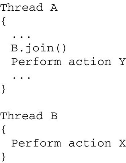
FIGURE 2.31 Pseudocode example showing the use of join primitive to synchronize threads.

Thread synchronization with join is explored in more detail in the Threads_Join program (see Figure 2.32).

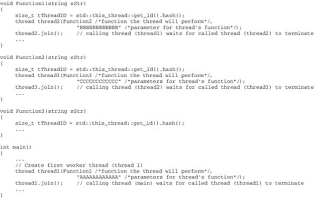
FIGURE 2.32 Selected code sections—Threads_Join example (C++).

Figure 2.32 shows the threading control parts of the Threads_Join sample program code. The main thread creates the first worker thread (thread1) and then joins the thread to itself. This causes the main thread to pause until thread1 terminates. Thread1 then creates thread2 and joins thread2 to itself, causing thread1 to pause until thread2 terminates. Similarly, thread2 creates thread3 and joins thread3 to itself; thus, thread2 pauses until thread3 terminates. The effect of this chain of joins is that the threads complete their work in the reverse order that they were created, thread 3 finishing first and the main thread finishing last. The synchronous behavior that arises is illustrated in Figure 2.33.

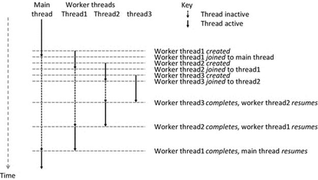
FIGURE 2.33 Synchronous behavior and thread execution order arising from the use of the join primitive in the Threads_Join sample program.

Alternatively, where there is no requirement of synchronized thread behavior, it may be desirable to allow all threads to run concurrently (as far as the process is concerned) and let the operating system schedule them freely, based on its thread scheduling mechanism. The detach primitive can be used to achieve this. detach() has essentially the opposite meaning to join(); it means that the calling thread should not wait for the called thread, but can instead run concurrently with it. This is illustrated in Figure 2.34, which shows the pseudocode for a scenario in which action X and action Y can be performed concurrently.

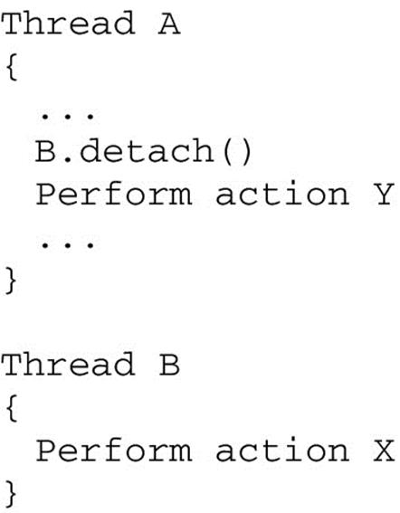
FIGURE 2.34 Pseudocode example of use of detach primitive to enable threads to run concurrently.

The use of detach to run threads asynchronously is explored in more detail in the Threads_Detach program (see Figure 2.35).

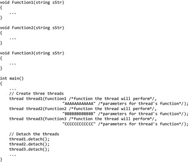
FIGURE 2.35 Selected code sections—Threads_Detach example (C++).

Figure 2.35 shows the threading control parts of the Threads_Detach sample program code. The main thread creates the three worker threads and then detaches all three of them from itself. This causes the threads to run asynchronously with respect to each other (the creating thread does not wait for the created threads to complete; instead, it is scheduled concurrently with them). This behavior is illustrated in Figure 2.36.

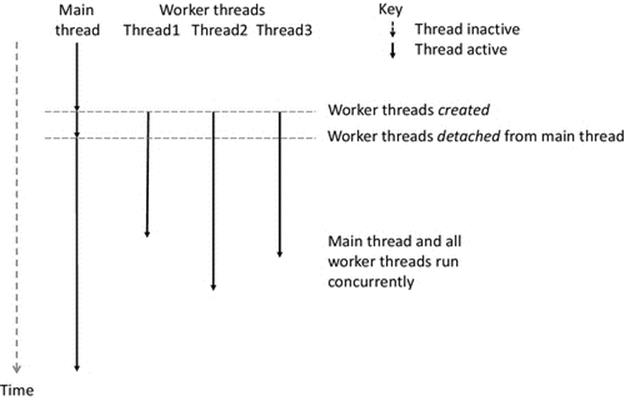
FIGURE 2.36 Asynchronous thread execution behavior arising from the use of the detach primitive in the Threads_Detach sample program.

Threads can relinquish the CPU when they have completed a particular task or when they need to wait for some other activity to be performed before continuing; this is called “yielding” and is performed by the relevant thread using the yield() primitive. However, the thread does not choose which thread runs next; this aspect is a scheduler function and is performed by the operating system based on the subset of other threads that are ready to run.

The use of the join() and detach() primitives to achieve synchronous and asynchronous thread behaviors, respectively, is investigated in Activity P11.

Activity P11

Empirical Investigation of the Behavior of Threads

Prerequisites

The instructions below assume that you have obtained the necessary supplemental resources as explained in Activity P1.

Learning Outcomes

1. To gain an understanding of threads concepts

2. To gain a basic understanding of the ways in which threads are used within programs

3. To gain a basic understanding of synchronous and asynchronous thread execution

Method

This activity uses a pair of programs Threads_Join and Threads_Detach to illustrate how created worker threads can be executed either synchronously or asynchronously. The activity is carried out in two parts.

Part 1. Executing Threads with the join() Operation

1. Examine the source code for the Threads_Join program. Make sure you understand the logic of this program, especially the way in which three threads are created, each inside the previous one (thread1 being created inside the main function, thread2 being created inside thread1, and thread3 being created inside thread2); in each case, the threads are “joined” with their creating thread.

2. Run the Threads_Join program in a command window. Navigate to the “ProcessView” subfolder and then execute the Threads_Join program by typing Threads_Join.exe followed by the Enter key.

3. Observe the behavior of the threads. Try to relate what you see happening to the logic of the source code.

The screenshots below provide examples of the thread execution patterns that occur. The left screen image shows the behavior when join() is used to synchronize the threads behavior—here, the calling thread (the one that uses the join primitive) waits for its called thread to finish before it continues (i.e., the threads run synchronously with respect to each other). The right screen image shows the behavior when detach() is used to start the threads—in this case, the threads run asynchronously.

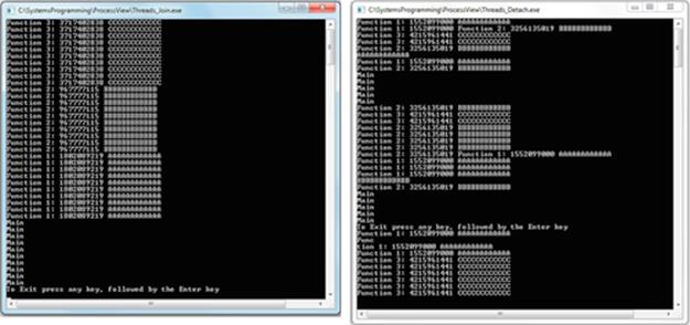
Part 2. Executing Threads with the detach() Operation

1. Use the same method as part 1, but this time using the Threads_Detach program.

2. You should see that the behavior is different each time you run the Threads_Detach program. You will see the outputs from the three threads are interlaced with each other and also with the outputs from main, which indicates they are all running in parallel (i.e., the calling thread does not wait for its called thread to finish before it continues).

Expected Outcome

You should see that the three threads are started as part of the same process, but the threads themselves execute their instructions independently of the other threads. You should see the different effects of using join() and detach() to determine whether the logic in the calling function should synchronize with the termination of the called thread or whether the threads can run concurrently. You should notice that the threads are assigned a unique ID (within the process itself) and that this ID is dynamically allocated and can change each time the program is run. You should also see that with detach(), the actual relative timing of the threads' behavior (and thus the ordering of their output) is not predictable and can differ each time the program is run.

Reflection

Threads are a means of ensuring responsiveness within programs, by having different “threads” of logic running independently, and in parallel with other threads. This not only introduces the potential for efficient operation but also can lead to overall behavior, which is hard to predict, especially with respect to timing, as this activity has shown, and thus emphasizes the need for careful design and testing.

This activity has illustrated the fundamental nature of threads, although it is important to point out that this is a simple example and that multithreaded applications can exhibit significantly more complex behavior than shown here.

2.7.5 Additional Complexity Accompanying Threading

A single thread of control is predictable, fundamentally because only one action (such as reading a variable or writing a variable) can occur at any time, and thus, the consistency of its private data space is ensured. However, with multiple threads sharing access to the process' data space, there is the possibility that the timing of different threads' actions will lead to inconsistencies. For example, if one thread writes to a variable and another reads the same variable, the precise timing of these actions becomes critical to ensure updates are performed in the correct order and that data values are not overwritten before they are used. This is an example of what is called “race conditions.” Without careful regulation, threaded applications are nondeterministic in the sense that the overall sequence of events and thus the actual behavior and results achieved are sensitive to the actual fine-grained timing behavior in the system, such that if the same process runs twice, it may give different results, even if the actual data values used are the same each time. The necessary regulation to ensure that processes' behavior remains deterministic, at least in terms of data consistency, and ultimately produces the correct result is achieved through the combination of careful program design and the use of run-time control mechanisms such as semaphores and the “mutex,” which provides mutually exclusive access to resources so that operations performed by different threads cannot overlap.

Even once the design is correct, the testing required to confirm correctness and consistency is itself complex because it must ensure that under all possible timing and sequencing behaviors, the end result remains correct. Erroneous use of mechanisms such as semaphores and mutexes and the join primitive can lead to deadlock situations in which all threads are blocked, each waiting for another thread to perform some action. The design stage should ensure that such problems cannot occur, but because of the complex timing relationships that can exist between multiple threads at run time, this aspect itself can be challenging. Thus, the design, development, and testing of multithreaded versions of applications can be significantly more complex than for single-threaded versions.

2.7.5.1 Application Scenarios for Multithreading

Multithreading can be used to enable a process to remain responsive despite IO activities. In a single-threaded program, if the single thread performs an IO activity such as reading a large file or waiting for a message from another process, as is a common scenario in distributed applications, the process itself is blocked by the scheduler. This has the undesirable effect that the application “freezes” and does not respond to user commands. If the code is designed such that the tasks that are likely to block are each within separate worker threads that run concurrently with each other, then the application can remain responsive to user input. For example, consider a fast-action networked game that has an event-driven graphical user interface, regularly sends and receives messages across a network, and also requires local access to images and movie clips, which are accessed as files from local secondary storage such as a hard disk. In such an application, a main nonfunctional requirement is high responsiveness to the user commands and the corresponding display updates; in fact, this would likely be a main determining factor as to the usability and user satisfaction rating of the game. Access to the hard drive to retrieve a file or waiting for messages to arrive over the network would interfere with the smooth and fast responsiveness of the user interface that is required. This is a situation where a multithreaded approach would be advantageous, as the user-interface servicing could operate asynchronously to the other IO activities.

However, the simpler game that is used as a case study throughout this book does not require access to the local secondary storage while the game is running. In this case, a multithreaded solution could still be used to perform the network IO on a separate thread to the user interface, but since it is not a fast-action game, with user events occurring on the time frame of several seconds rather than several within a single second, a simpler approach has been taken that involves a single-threaded solution with a nonblocking socket so that the message buffer can be inspected without the process having to wait if there is no message available. This achieves the appropriate level of responsiveness without the added design complexity of a multithreaded solution.

Multithreading is advantageous to maximally leverage the computational resources of a processor. In a parallel application, multiple worker threads will be created that each perform the same computation but work with different subsets of the data. If the application is run on a multicore platform (assuming the kernel-level threading model), its process can use as many cores as it has threads, subject to the operating system's scheduling policy. Even on a single-core platform, multithreading can boost the performance of such applications because individual threads are able to perform IO (causing them to block), while others within the same process continue to run.

2.7.6 A Multithreaded IPC Example

As discussed earlier, IPC is a form of IO, and thus while waiting for an incoming message, a process will block. Concurrent sending and receiving can be achieved at process level by having separate threads for each of the sending and receiving activities (thus allowing each to be scheduled, and blocked, independently). In this section, we use a multithreaded IPC example to extend the discussion of benefits of multithreading and also to delve a bit deeper into IPC issues.

The Multithreaded_IPC program combines threading and IPC and demonstrates how, by using asynchronous threading, the sending and receiving activities can operate concurrently. Note that in a single-threaded application, these would be serialized and the application would be difficult to use because each of the two activities would block while waiting for IO activities (the send activity waits for user input from the keyboard, while the receive activity waits for IPC messages to arrive on the socket). In contrast, the Multithreaded_IPC process waits for a message while continuing to send typed messages each time the user enters a new line. Send and receive are executed on separate threads, using blocking sockets. Separate sockets are used so that there are no race conditions within the process behavior. The program has two command-line arguments (send port and recv port) so that two instances of it can be configured to communicate together, as explained in Activity P12.

As illustrated in Figures 2.37 and 2.38, the receive function is placed into a worker thread, so when this thread blocks while waiting for an IPC message, it does not block the main thread. In this simple example, the sending activity is run on the main thread, as there is no business logic as such. In a more complex application with specific business logic, it would be possible to place the send activity in a further worker thread so that the business logic can operate while the send thread is blocked waiting for the user to type input; key sections of code concerned with the threading aspect are shown, with annotation, in Figures 2.39 (the main thread) and 2.40 (the receive thread).

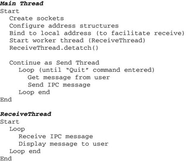
FIGURE 2.37 Pseudocode of the Multithreaded_IPC program.

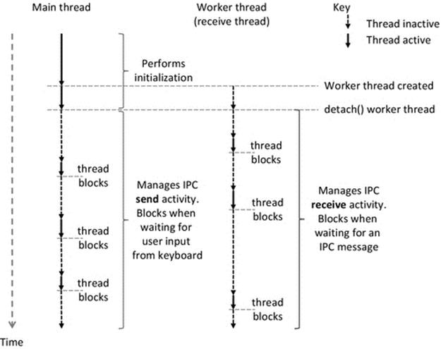
FIGURE 2.38 The main thread and worker thread run concurrently in Multithreaded_IPC.

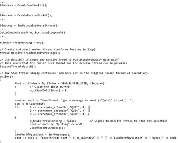
FIGURE 2.39 Annotated key sections of the Multithreaded_IPC program, main thread (C++ code).

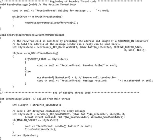
FIGURE 2.40 Annotated key sections of the Multithreaded_IPC program, receive thread (C++ code).

Activity P12 uses two process instances of the Multithreaded_IPC program to explore the asynchronous communication behavior achieved by the multithreaded design.

Activity P13 uses the “Threads—Introductory” simulation within the Operating Systems Workbench to explore the behavior of threads and to investigate the differences between synchronous and asynchronous thread execution.

Activity P12

Further Investigation of Threads and IPC Using the Multithreaded IPC Program

Prerequisites

The instructions below assume that you have obtained the necessary supplemental resources as explained in Activity P1.

Learning Outcomes

1. To reinforce understanding of threads concepts

2. To reinforce understanding of the use of sockets to achieve IPC

3. To gain an understanding of how asynchronous multithreading facilitates having concurrent blocking activities (in this case, send and receive), which would otherwise be serialized

Method

This activity uses two process instances of the program multithreaded IPC communicating together to illustrate full-duplex communication in which send and receive operate concurrently in each direction:

1. Examine the source code for the multithreaded IPC program. Make sure you understand the logic of this program, especially the way in which the communication activity is separated across the two threads (such that the main thread deals with sending functionality, while a worker thread is created to deal with receive functionality).

2. Run two instances of the program, each in a separate command window, remembering to swap the ports order in the command-line arguments so that the send port of the first instance is the same as the receive port for the second instance, and vice versa. For example,

3. Experiment with the two processes. Try to send and receive in various orders, to confirm that the process itself remains responsive, even when waiting for input from the keyboard or waiting for a message to arrive.

The screenshots below provide examples of the Multithreaded_IPC processes in action during the experiment. Note that the program logic is configured specifically by the port number parameters provided on the command line. Hence, the two processes shown below are communicating with each other using two separate unidirectional communication channels (at thread level) to provide bidirectional communication at the process level.

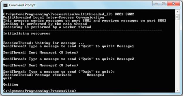
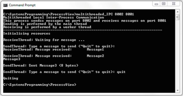
Expected Outcome

You should see that the two instances of the program work independently because they are separate processes individually scheduled by the operating system. They perform IPC via sockets and this communication works independently in each direction. The processes remain responsive because they use separate threads to perform the sending and receiving actions, and thus, these threads become blocked on an individual basis, as necessary.

Reflection

This activity provides an example of kernel-level threading. The send and receive threads each block when waiting for input. In the case of the receive thread, blocking occurs when it waits for a message to arrive from the other copy of the program. In the case of the main thread (which performs the send function), blocking occurs when waiting for the user to type a message on the keyboard that will be sent to the other copy of the program.

Activity P13

Using the Operating Systems Workbench to Explore the Behavior of Threads

Prerequisites

The instructions below assume that you have obtained the Operating Systems Workbench and the supporting documentation as explained in Activity P5.

Read the document “Threads (Introductory) Activities.”

Learning Outcomes

1. To enhance understanding of threads concepts

2. To enhance understanding of synchronous and asynchronous thread execution

Method

This activity uses the “Threads Introductory” simulation, which is found on the “Threads” tab of the Operating Systems Workbench. The simulation supports up to three threads running concurrently. The threads color randomly chosen pixels on a display area, each thread using a specific color (red, green, or blue) for the three threads, respectively. The progress of the threads can be visually followed by the color density of the screen area—so if the “red” thread receives more computational time than the other two, the “red intensity” will be higher than the green and blue intensities.

Part 1. Asynchronous Thread Scheduling (the Process Does Not Actively Control the Thread Execution Sequence)

1. Create and start a single thread. Notice how the thread gradually paints the (initially black) drawing area with its own color, the intensity of a particular pixel being incremented each time the pixel is randomly chosen. Leave this running for a few minutes or more and you should see near-total coloring.

2. Reset the drawing canvas. Create and start all three threads together with the same priority. Leave this running for a few minutes or more and you should see near-total coloring—which approximates to white—that is, an approximately even mix of red, green, and blue pixels.

3. Reset the drawing canvas. Create and start all three threads together; this time, set the threads to a mixture of highest and lowest priority (the differentiation between the other levels can be quite fine and the effect difficult to see). Leave this running for a few minutes or more and you should see the higher-priority thread(s) dominating with their color coverage.

Part 2. Synchronous Thread Scheduling (the Thread Execution Sequence Is Controlled Within the Process Itself)

1. Select the “Externally impose priority” radio button. Use the “Create and start threads” button to start the simulation with all threads having equal priority. You will notice that each thread runs for a short time in sequence, leading to a color-cycling effect. Experiment with different priorities of the threads (use the highest and lowest priorities to obtain the most visible effects). Notice that in this example, priority is translated into the share of run time that each thread gets, so the average color of the drawing area will be dominated by the colors attributed to the highest-priority thread(s).

The four screenshots below provide snapshots of the threads simulation for part 1 (in the sequence: top left, top right, bottom left, bottom right, respectively): only the red thread is running, the green thread has highest priority, the red and blue threads have highest priority, and, finally, all threads have equal priority.

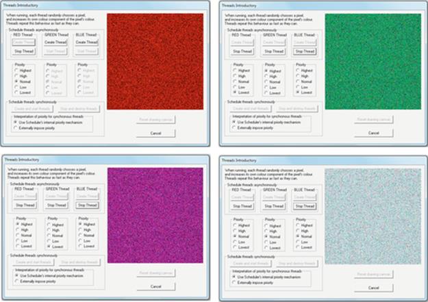
The screenshots below show the transition from red thread to green thread in part 2, on the left when all threads have equal priority and on the right when the red thread has lowest priority, and thus, the display remains mainly blue even after the red thread has run.

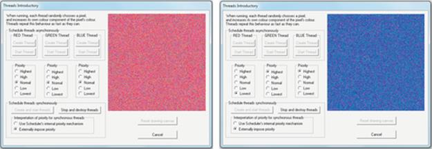
Expected Outcome

By having each thread draw in a different primary color, the simulation provides a means of visualization of the share of run time each thread receives.

In part 1, the threads run concurrently, and because the thread interleaving is very fast, they appear to run in parallel. You can see the resulting interleaving of pixel coloring behavior achieved.

Part 2 shows the effect of synchronous scheduling in which only one thread runs at any instant, leading to a color-cycling effect. It is important to realize that the amount of time for which each thread runs for has been exaggerated to ensure the effect works visually for the purpose of demonstration. In real systems that schedule threads in sequence, they may typically run for 10 s or perhaps 100 s of milliseconds at a time.

Reflection

This simulation illustrates the scheduling of threads within a process. There can be many processes in a system, as we have discussed earlier. Within each process, there can be many threads. The individual threads are scheduled entirely by the operating system itself in some systems and are controlled to some extent at the process level (by primitives in the process' code) in other systems.

From an application design viewpoint, try to think of situations where separate threads within a process is an appropriate solution, as opposed to having separate processes.

Further Exploration

Experiment further with the “Threads Introductory” simulation to gain a deeper understanding.

2.8 Other Roles of the Operating System

In addition to process scheduling as discussed in some detail above, operating systems need to perform a variety of related tasks. These arise from the need to manage the resources of the system and make them available to the processes that are running, as they are needed.

Two other roles are briefly identified here as they have impacts on the way that processes operate and the overall efficiency and effectiveness of the platforms on which the processes run. As these activities impact significantly on the use of resources, they are revisited in more detail in Chapter 4.

Memory management. The operating system must ensure that processes have access to a reserved area of memory for the duration of their execution. It must limit the amount of memory used by any single process and ensure that processes are separated from (and protected from) each other, by preventing one process from reading or modifying the part of memory currently in use by another process.

Resource allocation. Processes request access to certain resources dynamically, at times unpredictable (certainly to the operating system). The operating system must ensure that processes are granted resources as needed while maintaining separation of processes and preventing a conflict arising where two processes attempt to use a resource simultaneously. If a request for access to a resource is denied by the operating system, the process may wait (blocked).

2.9 Use of Timers Within Programs

There are many situations where tasks need to be executed periodically at a certain rate, and possibly, several different types of event or task need to occur at different rates within the same program. Timers provide a means of executing code within a process at a certain period or after a specific interval. These are particularly useful in distributed applications in combination with nonblocking sockets operations, for example, checking to see if a message has arrived, without blocking the application to wait for the message; this is discussed in depth in Chapter 3, and the use of timers is illustrated. Here, the concept of using timers is introduced for completeness as it has some similarities with and can be considered an alternative to using threads in some circumstances.

The expiry of a timer can be considered an event to which the program must respond. The function that is invoked is called the “event handler” for the timer event.

Activity P11 has introduced threads and has shown their main benefit, which is that the threads operate in parallel with each other, but this also reveals a potential weakness—it can be difficult to predict the sequence of operations across multiple threads and can be difficult to ensure that one specific event occurs before, or more frequently, than another. Timers allow blocks of code to execute asynchronously to the main function and can be a useful alternative to threads to ensure responsiveness without the potential complexity overheads that can arise with multithreaded solutions. The fundamental difference is that threads are scheduled by the operating system, and thus, the developer does not have control over their relative ordering or timing. Timers, on the other hand, cause their event handlers to be invoked at developer-decided intervals, and thus, the developer can embed precise timing relationships between events, into the program logic.

A simple example of the use of timer-based activity is an environment monitoring application, which has a temperature sensor and measures the temperature value at a fixed time interval. The Distributed Systems Workbench contains an example of this (the distributed temperature sensor application), which is discussed in Chapter 3.

Figure 2.41 illustrates the run-time sequencing of a program that performs three timer-based functions. The program's logic is initiated in its main function. Three programmable timers are set, and when each of these expire, its related function is invoked automatically. On completion of the function, control is returned to the main function at the point where it previously left off, in the same way that returning from a standard function call works. Annotated sections of the Timers_Demonstration program are provided in Figure 2.42.

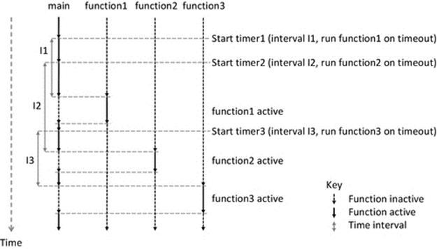
FIGURE 2.41 Timer-driven behavior.

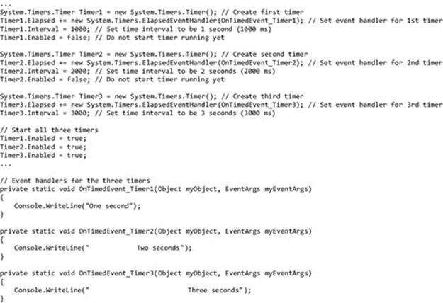
FIGURE 2.42 Annotated sections of the Timers_Demonstration c# program.

Figure 2.43 shows the output produced by the Timers_Demonstration process. The three timers run independently, effectively as separate threads, asynchronously with each other and the main thread. On close inspection of the output, you can see that at the point where 6 s have passed, all three timers expire at the same time, and in such a situation, it is not predictable by looking at the code which one will actually be serviced first. In this case, timer 3 is serviced first, followed by timer 2 and then timer1. Similarly, you can also see that after 2 s has passed, the second timer event handler is serviced before the first timer handler.

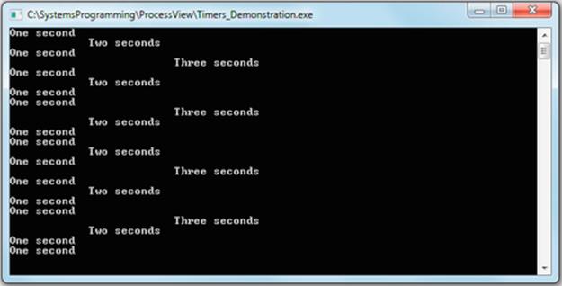
FIGURE 2.43 The Timers_Demonstration process running.

2.9.1 Use of Timers to Simulate Threadlike Behavior

It is possible to achieve threadlike behavior within a process by using timers and their event handlers to achieve multiple “threads” of control. The timer event handlers are similar to threads in the sense that they run independently of the other event handlers and also independently of the main thread of control. However, the main difference is that with timers, the actual timing of when the event handlers run is under the control of the programmer. This approach is better for periodic tasks within a process and can be used to achieve a real-time effect even without the use of a real-time scheduler (although the timing accuracy of the timers is not reliable for small time intervals, typically less than about 100 ms).

The timer countdown is managed by the operating system kernel, and thus, the countdown continues regardless of the whether the process is in the run state or not (i.e., the process is not itself decrementing the timer, this happens automatically as far as the process is concerned and the event handler is invoked automatically when the timer expires—which means its countdown reaches zero).

An example situation where I regularly use timers to achieve a threading-like behavior is in low-end embedded systems where the code runs “on the metal” (i.e., there is no operating system to manage resources). My application has to directly manage the resources it uses and natively runs as a single thread of control, following the various branches in the code based on a combination of the program logic and the contextual inputs from sensors. These systems have various hardware modules that can generate interrupts, including typically several programmable timers. Interrupt handlers have higher priority than the main thread of instruction execution, so I can create a high-priority “thread” by placing its logic in a timer interrupt routine and configuring the timer to interrupt at a suitable rate. For example, consider a sensor node application in which I need to have a general sensor monitoring application running as the foreground thread of control while periodically sampling a particular sensor at a certain rate (using one programmable timer) and also sending a status message to other sensor nodes at regular intervals (using a second programmable timer).

2.10 Transparency from the Process Viewpoint

Of the various forms of transparency that are required in distributed systems, two forms in particular are important from the process viewpoint. These are briefly introduced here and are treaded in more depth in Chapter 6.

2.10.1 Concurrency Transparency

In situations where multiple concurrent processes can access shared resources, the operating system must ensure that the system remains consistent at all times. This requires the use of mechanisms such as locks (discussed in Chapter 4) and transactions (discussed in Chapters 4 and 6) to ensure that processes are kept isolated from each other and do not corrupt each other's results, which would leave the system in an inconsistent state.

2.10.2 Migration Transparency

If a resource is moved while in use, any process using the resource must be able to continue to access it without any side effects; this is quite challenging. More commonly, resources are only moved when they are not in use, and then, directory services are updated so that the resources can be found in their new location.

Moving a running process is possible in some systems; it has been done in some load sharing schemes, for example. However, this is far more complex than moving a resource. To move a process, it must first be stopped (frozen), then its process state is captured and transferred to a new location, and the process is restarted running so that it continues from the place it left off. The process must not notice anything different; its state must have been preserved so that its computation will be consistent despite the move. This is analogous to a person being moved between identical hotel rooms while asleep, such that when they wake up, they see the same environment and pick up from where they left off unaware that they have been relocated.

2.11 The Case Study from the Process Perspective

The case study application is a game (tic-tac-toe) that is played across a network. The discussion below focuses on the process perspective, and the other aspects such as the networking and distribution and resource usage are discussed in the relevant other chapters.

The game application comprises two types of component: a client program and a server program. The client will run on each user's (game player's) computer, providing their interface to the game and enabling them to play the game remotely. The server will run on any computer in the network. It can be placed on one of the users' computers or can be on a separate computer. The server provides connectivity between the two clients (who do not communicate directly with each other) and also provides the control and synchronization of the game logic and stores the game state.

Running the game requires that the various components are run on the various computers. Note that there is only one client program, but this will be run on two computers, giving rise to two client process instances. The program logic of each of these is identical, but the actual behavior of these will be different because it is configured by the users inputs (in the game of noughts and crosses, this input includes the selection of which available space to place their token, at each turn).

The client processes will communicate with the server process using sockets as an IPC technique. The server will manage game state, and thus, when two clients are related through a live game, the server will mediate in terms of turn-taking by the users; so the server will enable one of the clients to enter a move while preventing the other.

2.11.1 Scheduling Requirements

The application has loose timing requirements in the sense that users expect their input to be processed promptly and the response time (in terms of updating both client user interfaces to reflect the latest move) should be low, perhaps within 1 s is acceptable.

The timing requirements are not precise; there are no specific deadlines and the time-bounded aspect is very weak with no real consequences. Some variance (arising, e.g., due to heavy workload at one or more of the host computers) is acceptable without diminishing user satisfaction appreciably; thus, the game is not in the soft real-time category.

Such timing requirements are typical of very many general-purpose user event-driven applications and should be serviced adequately by any of the currently used schedulers in popular operating systems, discussed earlier. There is no requirement for real-time scheduling.

2.11.2 Use of Timers

Programmable timers are required within the game application. A timer is used in both the client and server components to check for incoming messages at regular intervals of 100 ms. Essentially, the timer interrupt handler is used to run the receive functionality asynchronously with respect to the main thread, which handles the user interface and the send functionality (which is driven directly from the user input). By using a nonblocking socket for receive, in combination with the timer, which checks for received messages frequently, a responsive, multithreaded effect is achieved without actually requiring a multithreaded solution.

There are no time-dependent elements in the game logic itself.

2.11.3 Need for Threads

Client side: Due to the turn-based game play in this particular application, the user interface need not be highly responsive (compare, e.g., with a shoot 'em up-style game where the users are making command inputs and needing display updates at a very high rate). Given the style of game and the relatively low rate of user interaction with the interface, the user-interface aspect of the game client does not need to be multithreaded (whereas, for a fast-action game, this would be needed). A multithreaded solution is not required from the communication point of view because the communication timing requirement is not strict. The combination of a timer and nonblocking sockets lends itself to a simpler solution in this case.

Server side: The game server will support a small number of active games, and the message-load per active game is low; one message is received each time a client move is made, the server then having to compute the new game state and send a message to each of the two clients. Given the low rate of this operation and the low complexity of the game logic itself, the server need not be multithreaded.

However, the game logic could be redesigned as a multithreaded solution if required, for example, if a fast-action aspect with specific timing requirements were added to the game action or if more complex communication timing constraints were added. In such a case, it would be appropriate at the client side to separate send functionality and receive functionality each onto their own threads and have a third thread to handle the user-interface events.

The lack of requirement of multithreading at both client and server sides makes the game very suitable as a case study for the purposes of this book because the program operation is easy to understand, allowing the discussion to focus on the architecture, distribution, and communication aspects.

2.11.4 IPC, Ports, and Sockets

The IPC between processes in the game will take place across a network. While it is possible to run two clients at the same computer, it does not make sense from a distributed game point of view; it would imply that two players were sat at the same computer. The processes will use sockets as communication end points. The server will bind to a port whose number is known to, or discoverable by, client processes. Chapter 3 will deal with networking aspects in detail.

Figure 2.44 illustrates the structure of the game at various levels. This representation is very useful to help clarify the terminology we should use. It is important to recognize that the game itself is the application, which comprises two different programs: the client and server. These programs cannot really be called applications in their own right, because they do not do anything meaningful on their own; both parts are needed to actually play the game. This particular game is a two-player game, and therefore, the client program will need to run on two computers, one for each player. Note that the client program provides the user interface, which allows the user to interact with the game logic, which in this case actually resides on, and is controlled by, the server. The two players will require the same interface, and thus, both will use the same client program. It is very important to realize that an in-play instance of the game comprises two process instances of the single client program (i.e., not two different client programs). As the figure depicts, the IPC is between each client process and the server process. The IPC channels shown can be considered private communication between each pair of processes. When following the client-server paradigm, it is usual that the clients do not communicate directly. The combination of client-server game architecture and socket-based IPC gives rise to two hardware configurations, that is, two different mappings between the processes and the computers they run on. The first of these is that each process can reside on a separate computer. However, only the location of the clients is important (i.e., their location depends on where the actual players are), but the server can be anywhere in the network and thus can also be on the same computer as one of the clients. Technically, it would be possible to put all three processes on the same computer, and in some applications, this might make sense, but this mapping is not applicable in a two-player game in which each player needs their own keyboard and screen in order to interact with the game.

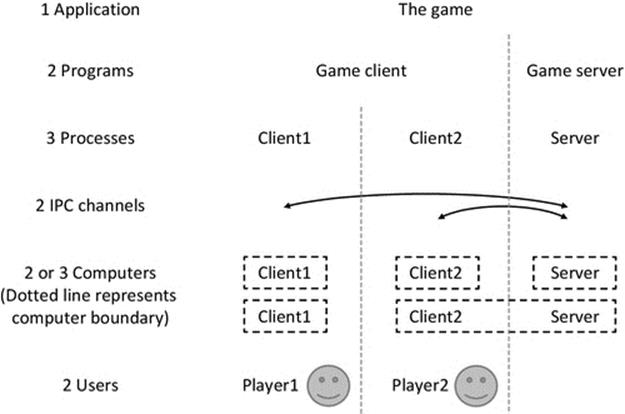
FIGURE 2.44 Structural mapping of the components of the game, at the various levels.

Figure 2.44 also helps to reinforce the very important concept that a server is a process, and not a computer. A common misconception is that a server is a computer; this arises because often, a dedicated computer is provisioned to run a particular service (i.e., to house a server process) and then the computer itself gets referred to as “the server”; but as illustrated in the figure, the server is very clearly a process and in fact could be moved from one computer to another without affecting the way in which the game works.

2.12 End-of-Chapter Exercises

2.12.1 Questions

1. Consider a single-core processor system with three active processes {A, B, C}. For each of the process state configurations a-f below, identify whether the combination can occur or not. Justify your answers.

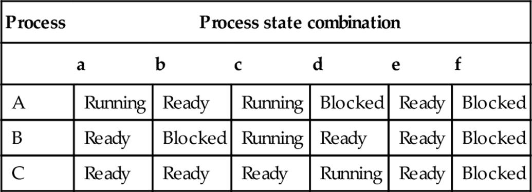
2. For a given process, which of the following state sequences (a-e) are possible? Justify your answers.

(a) Ready → Running → Blocked → Ready → Running → Blocked → Running

(b) Ready → Running → Ready → Running → Blocked → Ready → Running

(c) Ready → Running → Blocked → Ready → Blocked → Ready → Running

(d) Ready → Blocked → Ready → Running → Blocked → Running → Blocked

(e) Ready → Running → Ready → Running → Blocked → Running → Ready

3. Consider a compute-intensive task that takes 100 s to run when no other compute-intensive tasks are present. Calculate how long four such tasks would take if started at the same time (state any assumptions).

4. A non-real-time compute-intensive task is run three times in a system, at different times of the day. The run times are 60, 61, and 80 s, respectively. Given that the task performs exactly the same computation each time it runs, how do you account for the different run times?

5. Consider the scheduling behavior investigated in Activity P7.

(a) What can be done to prevent real-time tasks from having their run-time behavior affected by background workloads?

(b) What does a real-time scheduler need to know about processes that a general-purpose scheduler does not?

2.12.2 Exercises with the Workbenches

Use the Operating Systems Workbench to investigate process scheduling behavior.

The following exercises are based on the “Scheduling Algorithms—Advanced” simulation within the Operating Systems Workbench.

Exercise 1. Comparison of the SRJN and RR scheduling algorithms. Both SRJN and RR are preemptive. The objective of this activity is to compare the efficiency and fairness of the two algorithms

1. Configure the simulation as follows:

Process 1: Type = CPU Intense, Runtime = 40 ms

Process 2: Type = CPU Intense, Runtime = 40 ms

Process 3: Type = CPU Intense, Runtime = 40 ms

Process 4: Type = IO Intense, Runtime = 30 ms

Process 5: Type = IO Intense, Runtime = 30 ms

IO Device Latency = 10 ms

Quantum Size = 10 ms
Scheduler Configuration = Round Robin

2. Run the simulation and KEEP A RECORD OF ALL THE STATISTICS VALUES.

3. Modify the configuration as follows:
Scheduler Configuration = Shortest Remaining Job Next

4. Run the simulation and KEEP A RECORD OF ALL THE STATISTICS VALUES.
Less CPU idle time implies better scheduling efficiency.

Q1. Which algorithm was more efficient in these simulations? Is this difference due to a carefully chosen set of processes, or will it apply generally?

A “fair” scheduler will give roughly similar waiting times to all processes.

Q2. Which algorithm was fairest in these simulations? Is this difference due to a carefully chosen set of processes, or will it apply generally?

Low waiting time and low “total time in the system” are measures of the responsiveness of processes.

5. Calculate the mean waiting time and mean total time in the system for the set of processes, for each simulation.

Q3. Which algorithm gave rise to the highest responsiveness of the processes in these simulations? Is this difference due to a carefully chosen set of processes, or will it apply generally?

Exercise 2. Investigation of the effects of changing the size of the Scheduling Quantum

1. Configure the simulation as follows:

Process 1: Type = CPU Intense, Runtime = 40 ms

Process 2: Type = Balanced, Runtime = 50 ms

Process 3: Type = IO Intense, Runtime = 40 ms

Process 4: Type = Balanced, Runtime = 30 ms

Process 5: Type = IO Intense, Runtime = 30 ms

IO Device Latency = 10 ms

Scheduler Configuration = Round Robin
Quantum Size = 5 ms

2. Run the simulation and KEEP A RECORD OF ALL THE PROCESS STATISTICS VALUES.

3. Modify the configuration as follows:
Quantum Size = 10 ms

4. Run the simulation and KEEP A RECORD OF ALL THE PROCESS STATISTICS VALUES.

5. Modify the configuration as follows:
Quantum Size = 15 ms

6. Run the simulation and KEEP A RECORD OF ALL THE PROCESS STATISTICS VALUES.

7. Modify the configuration as follows:
Quantum Size = 20 ms

8. Run the simulation and KEEP A RECORD OF ALL THE PROCESS STATISTICS VALUES.

9. Modify the configuration as follows:
Quantum Size = 25 ms

10. Run the simulation and KEEP A RECORD OF ALL THE PROCESS STATISTICS VALUES.

Q1. How does the quantum size affect fairness (i.e., which quantum size causes the processes to encounter similar wait times and which quantum size causes the greatest difference in the wait times)? Why is this so?

11. For each set of results, calculate the mean wait time and the mean total time in the system for the processes.

Q2. How does the quantum size affect the mean wait time? Why is this so?

Q3. How does the quantum size affect the mean total time in the system? Why is this so?

Exercise 3. Investigation of the effects of changing the IO device latency

1. Configure the simulation as follows:

Process 1: Type = CPU Intense, Runtime = 40 ms

Process 2: Type = Balanced, Runtime = 50 ms

Process 3: Type = IO Intense, Runtime = 40 ms

Process 4: Type = Balanced, Runtime = 30 ms

Process 5: Type = IO Intense, Runtime = 30 ms

Quantum Size = 15 ms
Scheduler Configuration = Round Robin
IO Device Latency = 5 ms

2. Run the simulation and KEEP A RECORD OF ALL THE PROCESS STATISTICS VALUES.

3. Modify the configuration as follows:
IO Device Latency = 10 ms

4. Run the simulation and KEEP A RECORD OF ALL THE PROCESS STATISTICS VALUES.

5. Modify the configuration as follows:
IO Device Latency = 15 ms

6. Run the simulation and KEEP A RECORD OF ALL THE PROCESS STATISTICS VALUES.

7. Modify the configuration as follows:
IO Device Latency = 20 ms

8. Run the simulation and KEEP A RECORD OF ALL THE PROCESS STATISTICS VALUES.

9. Modify the configuration as follows:
IO Device Latency = 25 ms

10. Run the simulation and KEEP A RECORD OF ALL THE PROCESS STATISTICS VALUES.

Q1. As IO device latency increases, what happens to the total time in the system (the time it takes to execute to completion) of each process?

Do any of the processes take longer to execute? If so, why?
Do any of the processes take less time to execute? If so, why?

11. For each set of results, calculate the mean wait time and the mean total time in the system for the processes.

Q2. How does the IO device latency affect the mean total time in the system? Why is this so? Is this what you expected?

Q3. How does the IO device latency affect the mean wait time? Why is this so (think carefully)? Is this what you expected?

Exercise 4. Predict and Analyze the behavior of the SRJN scheduling algorithm (part 1)

1. Configure the simulation as follows:

Process 1: Type = Balanced, Runtime = 40 ms

Process 2: Type = Balanced, Runtime = 50 ms

Process 3: Type = IO Intense, Runtime = 30 ms

Process 4: Type = Not selected

Process 5: Type = Not selected

IO Device Latency = 20 ms
Quantum Size = 10 ms
Scheduler Configuration = Shortest Remaining Job Next0

Q1. Predict which process will finish first.

Q2. Predict which process will finish last.

Q3. Predict how much time process 1 will spend in the blocked state.

2. Run the simulation to check your predictions. If you were wrong, make sure that you understand why.

3. Modify the configuration as follows:

Process 1: Type = CPU Intense, Runtime = 70 ms

Process 2: Type = Balanced, Runtime = 50 ms

Process 3: Type = IO Intense, Runtime = 30 ms

Process 4: Type = Not selected

Process 5: Type = Not selected

Q4. Predict which process will finish first.

Q5. Predict which process will finish last.

Q6. Predict how much time process 1 will spend in the blocked state.

4. Run the simulation to check your predictions. If you were wrong, make sure that you understand why.

Exercise 5. Predict and Analyze the behavior of the SRJN scheduling algorithm (part 2)

1. Configure the simulation as follows:

Process 1: Type = IO Intense, Runtime = 40 ms

Process 2: Type = IO Intense, Runtime = 50 ms

Process 3: Type = CPU Intense, Runtime = 100 ms

Process 4: Type = IO Intense, Runtime = 30 ms

Process 5: Type = IO Intense, Runtime = 40 ms

Quantum Size = 25 ms
Scheduler Configuration = Shortest Remaining Job Next
IO Device Latency = 25 ms

Q1. Predict which process will start first.

Q2. Predict which process will finish first.

Q3. Predict which process will finish last.

Q4. Predict how much time process 1 will spend in the blocked state.

Q5. Predict how much time process 4 will spend in the run state.

2. Run the simulation to check your predictions. If you were wrong, make sure that you understand why.

3. Modify the configuration as follows:
IO Device Latency = 20 ms

Q6. Predict which process will start first.

Q7. Predict which process will finish first.

Q8. Predict which process will finish last.

Q9. Predict how much time process 2 will spend in the blocked state.

Q10. Predict how much time process 3 will spend in the run state.

4. Run the simulation to check your predictions. If you were wrong, make sure that you understand why.
The following exercise is based on the “Real-Time Scheduling Algorithms—Advanced” simulation within the Operating Systems Workbench.

Exercise 6. In-depth comparison between the RATE MONOTONIC (RM) and DEADLINE (DL) scheduling algorithms

Using each of the following process configurations, experiment with the two scheduling algorithms. Keep detailed notes of behavioral characteristics and any “interesting” observations or problems that occur. The goal is to perform a scientific comparison of the two scheduling algorithms.

Configuration A:

Process 1: Inter-arrival 30, Computation time 12, Start delay 0, and infinite tasks.

Process 2: Inter-arrival 20, Computation time 10, Start delay 0, and infinite tasks.

Process 3: Inter-arrival 25, Computation time 2, Start delay 0, and infinite tasks.

Configuration B:

Process 1: Inter-arrival 33, Computation time 16, Start delay 0, and infinite tasks.

Process 2: Inter-arrival 20, Computation time 10, Start delay 0, and infinite tasks.

Process 3: Inter-arrival 25, Computation time 2, Start delay 0, and infinite tasks.

Configuration C:

Process 1: Inter-arrival 33, Computation time 11, Start delay 0, and infinite tasks.

Process 2: Inter-arrival 33, Computation time 11, Start delay 0, and infinite tasks.

Process 3: Inter-arrival 33, Computation time 11, Start delay 0, and infinite tasks.

Configuration D:

Process 1: Inter-arrival 33, Computation time 6, Start delay 0, and infinite tasks.

Process 2: Inter-arrival 5, Computation time 2, Start delay 0, and infinite tasks.

Process 3: Inter-arrival 5, Computation time 2, Start delay 0, and infinite tasks.

Configuration E:

Process 1: Inter-arrival 30, Computation time 12, Start delay 0, and infinite tasks.

Process 2: Inter-arrival 20, Computation time 10, Start delay 0, and infinite tasks.

Process 3: Inter-arrival 25, Computation time 5, Start delay 50, and 5 tasks.

Configuration F:

Process 1: Inter-arrival 30, Computation time 13, Start delay 0, and infinite tasks.

Process 2: Inter-arrival 20, Computation time 10, Start delay 0, and infinite tasks.

Process 3: Inter-arrival 25, Computation time 5, Start delay 50, and 5 tasks.

When you have performed the comparative simulations, try these questions (in each case, justify your answer based on simulation evidence):

1. Which algorithm is the overall best for meeting task deadlines?

2. Which algorithm is the overall best for achieving high CPU utilization?

3. Do short-lived processes (those that have only a few tasks) interfere with/mess up the scheduling, or do the algorithms cope sufficiently?

4. Which is the overall best algorithm for REAL-TIME scheduling?

5. Are there any circumstances in which the overall-worst algorithm has advantages?

6. Is it possible to state that one algorithm is ALWAYS better than the other?

2.12.3 Programming Exercises

Programming Exercise #P1: Creating a bidirectional socket-based IPC application (extend the provided sample code to send a message and return a reply between a pair of processes).

Step 1: Examine the source code for the IPC_socket_Sender and IPC_socket_Receiver programs, which comprise the introductory sockets application we used in Activity P10.

Step 2: Rearrange the existing programs to create a new version of the application in which the original message sent to the receiver (which is sent to port 8007) is modified and sent back to the original sender (this time using port 8008). The modification can be something simple such as reversing the order of the characters in the message.

The main modifications you need to perform for the new sender program are the following:

• Create a new socket for receiving the reply message.

• Create a new socket address structure, which contains the address of the local computer and the port number 8008.

• Bind the new receiving socket to the local address structure.

• After the current send statement, add a receive statement, using the new receiving socket, which will wait for the reply message.

• Display the received reply message on the console output.

Note that all of the codes for these steps already exist in the original receiver program. The various sections of code can be copied into the new Sender program, with only minor changes needed.

The main modifications you need to perform for the new Receiver program are the following:

• Create a new socket for sending back the reply message.

• Modify the existing receive method, so that it stores the address of the message sender process.

• Create a new socket address structure, which contains the address of the sender process (so a reply can be sent back to it) and the port number 8008.

• Write a method to reverse the received message (or perform some other simple translation).

• After the current receive statement, add a send statement, using the new sending socket, to send back the reply message to the sender of the first message.

Note that all of the code for these steps already exists in the original Sender program. The various sections of code can be copied into the new Receiver program, with only minor changes needed.

A sample solution to this problem is provided in the programs IPC_socket_Sender_with_Reply and IPC_socket_Receiver_with_Reply.

Programming Exercise #P2: The Multithreaded_IPC program runs the receive activity as a worker thread, while the main thread performs the send activity. Rearrange the code so that both the sending and receiving activities are run on worker threads, and thus, the main thread is left free for other activity (which, in a real application, could be the core business logic).

To achieve this you, will need to refactor the code so that the sending activity is run as a separate thread, using detach() so that the new thread runs asynchronously with the main thread.

An example solution is provided in the application Multithreaded_IPC_two_worker_threads.

Programming Exercise #P3: The Multithreaded_IPC program shuts down the local process when the command “Quit” is entered. Modify the program so that in addition to this local shutdown, the remote communicating process is also shutdown.

To achieve this, you will need to send the message “Quit” across the network to the other process and then perform the local “quit” action. You also need to modify the receive logic so that the process shuts down if the command “Quit” is received from the socket communication, in the same way that at present it operates if the command is seen from the local user input.

An example solution is provided in the application Multithreaded_IPC_remote_shutdown.

2.12.4 Answers to End-of-Chapter Questions

Q1. Answer

Assuming a single-core processor system, at most, one process can be in the running state at any time:

Configurations a, d, and f are possible.

Configurations b and e can only exist momentarily because there are processes in the ready state and the CPU is not being used, so the scheduler should immediately dispatch one of the ready-state processes.

Configuration c cannot occur because there is only a single processing core.

Q2. Answer

Sequence a is not possible because a blocked to running transition is not allowed.

Sequence b is possible.

Sequence c is not possible because a process in the ready state cannot become blocked.

Sequence d is not possible because a process in the ready state cannot become blocked and because a blocked to running transition is not allowed.

Sequence e is not possible because a blocked to running transition is not allowed.

Q3. Answer

Four times as much CPU processing time is needed. So if the first task had received 100% of the CPU, then we can expect the four tasks to take 400 s, as each is now getting 25% of the CPU resource. If however the original task had received a share of the CPU resource less than 100%, then the calculation is more complex—for example, refer back to Activity P4 in which the first task gets 50% but when four run, they get 25% each. In such a case, we would expect the run time to be approximately 200 s when all four tasks run at once.

Q4. Answer

Non-real-time tasks are not guaranteed to run in any particular time period. Therefore, variation in actual execution times is the norm, not an exception. The variations arise because of the presence of other processes in the system, which compete for the processing resource. The scheduler makes short-term decisions as to which process to run based on the set of processes present and their individual process states. The state of the system as a whole is in constant flux as processes arrive, perform their work, and then complete; and so it is unlikely that the exact same conditions apply for more than a short sequence of consecutive scheduling decisions.

The minimum execution time can be achieved for a particular process only when it is given exclusive access to the CPU. In this case, the 60 s run time could be the minimum execution time, but there is not enough information provided to confirm this.

Q5. Answer

Part (a) A real-time scheduler that takes periodicity or deadlines into consideration is needed.

Part (b) Deadline of processes or either deadline or periodicity of subtasks generated by the process.

2.12.5 List of In-text Activities

2.12.6 List of Accompanying Resources

The following resources are referred to directly in the chapter text, the built-in activities, and/or the end-of-chapter exercises.

• Operating Systems Workbench (“systems programming” edition)

• Source code (including solutions to programming tasks)

• Executable code