Systems Programming: Designing and Developing Distributed Applications, FIRST EDITION (2016)

Chapter 4. The Resource View

Abstract

This chapter examines the resource aspects of distributed systems. It is concerned with ways in which resource availability and resource usage impact on communication and on the performance of the communicating processes. The main physical resources of interest are processing power, network communication bandwidth, and memory. The discussion focuses on the need to use these resources efficiently as they directly impact on performance and scalability of applications and the system itself. The characteristics and behavior of network protocols and transmission mechanisms are examined with particular emphasis on the way messages are passed across networks and the ways in which congestion can build up and the effects of congestion on distributed applications.

Memory is discussed in terms of its use as a resource for general processing and more specifically in the context of its use to provide buffers for the assembly and storage of messages prior to sending (at the sender side) and for holding messages after receipt (at the receiver side) while the contents are processed. The memory hierarchy is discussed in terms of the trade-offs between access, availability, and IO latency and the way in which program design can impact on efficiency and performance in this regard. Memory management is examined, in particular in terms of the use of virtual memory to extend the effective size of the physical memory available.

A number of virtual resource types, including sockets and ports, are discussed in terms of their relationship to processes and the management of communication.

Ways in which the design of distributed applications impacts on resource usage and efficiency are discussed, and the case study is examined from the resource perspective.

Keywords

Resource management

Memory buffer

Memory hierarchy

Virtual memory

Page replacement algorithms

Dynamic memory allocation

Shared resources

Lost updates

Transactions

Locks

Deadlock

Resource replication

Network bandwidth

Data compression

Serialization

Protocol data units

Encapsulation

Routing

Data consistency

Replication

4.1 Rationale and Overview

A computer system has many different types of resource to support its operation; these include the central processing unit (CPU) (which has a finite processing rate), memory, and network bandwidth. Different activities use different combinations and amounts of resources. All resources are finite, and for any activity, there will often be one particular resource that is more limited than the others in terms of availability and thus acts as a bottleneck in terms of performance. Resource management therefore is a key part of ensuring system efficiency, and it is thus necessary for the developers to understand the distributed applications they build in terms of the resources they use. It is also very important from a programming viewpoint to understand the way resources such as message buffers are created and accessed. This chapter presents a resource-oriented view of communication between processes, with a focus on how the resources are used by applications and the way the resources are managed, either by the operating system or implicitly through the way applications use them.

4.2 The CPU as a Resource

The CPU is a very important resource in any computer system, because no work can be done without it. A process can only make progress when it is in the running state, that is, when it is given access to the CPU. The other main resources (memory and network) get used as a result of process executing instructions.

Even when there are several processing cores available in a system, they are still a precious resource that must be used very efficiently. As we investigated in Chapter 2, there can be very many processes active in a modern multiprocessing system, and thus, the allocation of processing resource to processes is a key aspect that determines the overall efficiency of the system.

The Chapter 2 has focused mainly on the CPU in terms of resources. In particular, we looked at the way in which the processing power of the CPU has to be shared among the processes in the system by the scheduler. We also investigated the different types of process behavior and how competition for the CPU can affect the performance of processes. This chapter therefore focuses mainly on the memory and network resources.

However, the use of the various resources is intertwined; their use is not orthogonal. A process within a distributed system that sends a message to another process actually uses many resource types simultaneously. Almost all actions in a distributed system involve the main resource types (CPU, memory, and network) and virtual resources such as sockets and ports to facilitate communication.

For example, when dealing with memory as a resource, it is important to realize that the CPU can only directly access the contents of its own registers and the contents of random-access memory (RAM). Other possibly more abundant memory types, such as hard disk drives and USB memory sticks, are accessed with significantly higher latency as the data must be moved into RAM before being accessed. This illustrates the importance of understanding how the resources are used and the interaction between resources that occurs, which in turn is necessary in order to be able to make good design decisions for distributed applications and to be able to understand the consequences of those design decisions.

Poor design leading to inefficient resource usage can impact the entire system, beyond a single application or process. Negative impacts could arise, for example, in the form of network congestion, wasted CPU cycles, or thrashing in virtual memory (VM) systems.

4.3 Memory as a Resource for Communication

Consider the very simple communication scenario between a pair of processes in which a single message is to be sent from one process to the other. Several types of resource are needed to achieve this, so let us first look at the use of memory.

In order to be able to send a message, the sending process must have access to the message; that is, it must have been defined and stored in memory accessible to the process. The normal way to arrange this is to reserve a block of memory specially for holding a message prior to sending; we call this the send buffer or transmission buffer. A message can then be placed into this buffer for subsequent transmission across the network to the other processes.

A buffer is a contiguous block of memory, accessible by the process that will read and write data to/from it. The process may be part of a user application or may be part of the operating system. By contiguous, we mean that the memory must be a single unbroken block. For example, there must not be a variable stored in the same block of memory. In fact, we say that the block of memory is “reserved” for use as the buffer (of course, this requires sensible and informed behavior on the part of the programmer).

There are three significant attributes of a buffer (start address, length, and end address), as illustrated in Figure 4.1.

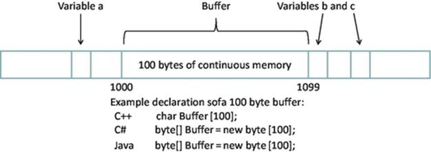
FIGURE 4.1 Illustration of a buffer; the one illustrated is 100 bytes long starting at address 1000 and ending at address 1099. Suitable declaration statements for some popular languages are also shown.

A buffer can be described precisely by providing any two of its three attributes, and the most common way to describe a buffer is by using start address and length. As each address in memory has a unique address and the memory used by the buffer must be in a contiguous block as discussed above, this description precisely and uniquely describes a particular block of memory. For the example shown in Figure 4.1, this is 1000 and 100. This information can be passed to the communication part of the application process; in the case of the sender, this indicates where the message that must be sent is stored, or in the case of the receiver, this indicates where to place the arriving message. Figure 4.1 also illustrates the requirement that the buffer's memory must be reserved such that no other variables overlap the allocated space. It is very important to ensure that accesses to the buffer remain within bounds. In the example shown, if a message of more than 100 bytes were written into the buffer, the 101st character would actually overwrite variable b.

The first resource-related issue we come across here is that the size of the buffer must be large enough to hold the message. The second issue is how to inform the code that performs the sending where the buffer is located and the actual size of the message to send (because it would be very inefficient to send the entire buffer contents if the message itself were considerably smaller than the buffer size, which would waste network bandwidth).

Figure 4.2 illustrates the situation where a message of 21 bytes is stored into a buffer of 40 bytes in size. From this figure, we can see several important things. Firstly, each byte in the buffer has an index that is its numerical offset from the start of the buffer, so the first byte has an index of 0, the second byte an index of 1, and so on, and perhaps, the most important thing to remember when writing code that uses this buffer is that the last byte has an offset of 39 (not 40). We can also see that each character of the message, including spaces, occupies one byte in the buffer (we assume simple ASCII encoding in which each character code will always fit into a single byte of memory). We can also see that the message is stored starting from the beginning of the buffer. Finally, we can see that the message in this case is considerably shorter than the buffer, so it is more efficient to send across the network only the exact number of bytes in the message, rather than the whole buffer contents.

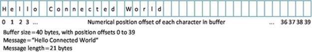
FIGURE 4.2 Buffer and message size.

A single process may have several buffers; for example, it is usual to have separate buffers for sending and receiving to permit simultaneous send and receive operations without conflict.

For many years, memory size was a limiting factor for performance in most systems due to the cost and the physical size of memory devices. Over the last couple of decades, memory technology has advanced significantly such that modern multiprocessing systems have very large memories, large enough to accommodate many processes simultaneously. The operating system maintains a memory map that keeps track of the regions of memory that have been allocated to each process and must isolate the various processes present in the system from each other. In particular, each process must only have access to its allocated memory space and must not be able to access memory that is owned by another process.

Each process is allocated its own private memory area at a specific location in the system memory map. Processes are unaware of the true system map and thus are unaware of the presence of other processes and the memory they use. To keep the programming model simple, each process works with a private address range, which starts from address 0 as it sees it (i.e., the beginning of its own address space), although this will not be located at the true address 0 at the system level. The true starting address of a process' memory area is used as an offset so that the operating system can map the process' address spaces onto the real locations in the system memory. Using the private address space, two different processes can both store a variable at address 1000 (as they see it). This address is actually address 1000 relative to the offset of where the process' memory begins; thus, its true address is 1000 plus the process' memory offset in the system memory address space; see Figure 4.3.

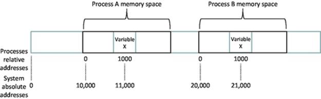
FIGURE 4.3 Process memory offsets and relative addressing.

Figure 4.3 illustrates the way in which different processes are allocated private memory areas with offsets in the true address range of the system and the way in which relative addressing is used by processes within their allocated memory space. This permits two process instances of the same program to run on the same computer, each storing a variable X at relative address 1000. The operating system stores the offsets for the two memory spaces (in this example, 10,000 and 20,000), thus using the true memory address offsets for each of the processes; the true locations of the two variables are known to the operating system (in this example, 11,000 and 21,000). This is a very important mechanism because it means that the relative addresses used within a program are independent of where the process is loaded into the true physical memory address range; which is something that cannot be known when the program is compiled.

Next, let us consider what information is needed to represent the size and location of a buffer within the address space of a particular process and thus the size and location of the message within it.

Figure 4.4 shows how the buffer is located within the process' memory space. Note here that the memory address offsets of the 10,000 bytes are numbered 0 through 9999 and that address 10,000 is not actually part of this process' memory space.

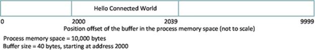
FIGURE 4.4 A buffer allocated within a process' address space.

The message starts at the beginning of the buffer (i.e., it has an offset of 0 within the buffer space) and has a length of 21 bytes. Therefore, by combining our knowledge of the message position in the buffer and our knowledge of the buffer position in the process' memory space, we can uniquely identify the location of the message within the process' memory space. In this case, the message starts at address 2000 and has a length of 21 bytes. These two values will have to be passed as parameters to the send procedure in our code, so that it can transmit the correct message.

We now consider the role of memory buffers in the complete activity of sending a message from one process (we shall call the sender) to another process (we shall call the receiver). The sender process must have the message stored in a buffer, as explained above, before it can send the message. Similarly, the receiver process must reserve a memory buffer in which to place the message when it arrives. Figure 4.5 provides a simplified view of this concept.

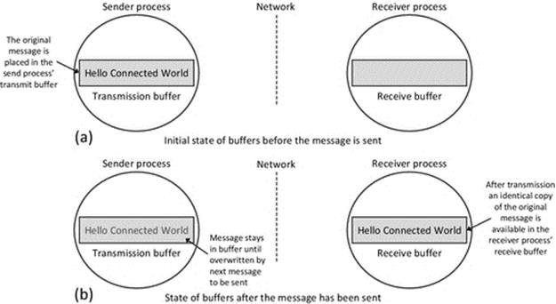
FIGURE 4.5 Simplified view of sender and receiver use of buffers.

Figure 4.5 shows the role of memory buffers in communication, in a simplified way. Part (a) of the figure shows the situation before the message is sent. The message is stored in a buffer in the memory space of the sending process, and the buffer in the receiving process is empty. Part (b) of the figure shows the situation after the message has been sent. The essential point this figure conveys is that the sending of a message between processes has the effect of transferring the message from a block of memory in the sender process to a block of memory in the receiver process. After the transfer is complete, the receiver can read the message from its memory buffer, and it will be an exact replica of the message the sender had previously placed in its own send buffer.

As stated above, this is a simplified view of the actual mechanism for the purpose of establishing the basic concept of passing a message between processes. The message is not automatically deleted from the send buffer through the action of sending; this is logical because it is possible that the sender may wish to send the same message to several recipients. A new message can be written over the previous message when necessary, without first removing the earlier message. The most significant difference between Figure 4.5and the actual mechanism used is that the operating system is usually responsible for receiving the message from the network and holding it in its own buffer until the recipient process is ready for it, at which point the message is transferred to the recipient process' receive buffer.

The receive mechanism is implemented as a system call that means that the code for actually performing the receive action is part of the system software (specifically the TCP/IP protocol stack). This is important for two main reasons: Firstly, the system call mechanism can operate when the process is not running, which is vital because it is not known in advance exactly when a message will arrive. The receiver process is only actually running when it is scheduled by the operating system, and thus, it may not be in the running state at the moment when the message arrives (in which case, it would not be able to execute instructions to store the message in its own buffer). This is certain to be the case when the socket is configured in “blocking” mode that means that as soon as the process issues the receive instruction, it will be moved from the running state to the blocked state and stays there until the message has been received from the network. Secondly, the process cannot directly interact with the network interface because it is a shared resource needed by all processes that perform communication. The operating system must manage sending and receiving at the level of the computer itself (this corresponds to the network layer). The operating system uses port numbers, contained in the message's transport layer protocol header to determine which process the message belongs to. This aspect is discussed in depth in Chapter 3, but the essence of what occurs in the context of the resource view is shown in Figure 4.6.

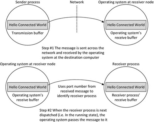
FIGURE 4.6 A message is initially received by the operating system at the destination computer and then passed to the appropriate process.

The most important aspect of Figure 4.6 is that it shows how the operating system at the receiving node decouples the actual sending and receiving processes. If the receiving process were guaranteed to be always running (in the running state), then this decoupling may be unnecessary, but as we have seen in Chapter 2, the receiving process may actually only be in the running state for a small fraction of the total time. The sending process cannot possibly synchronize its actions such that the message arrives at exactly the moment the recipient process is running, because, among other things, the scheduling at the receiving node is a dynamic activity (and thus, the actual state sequences are not knowable in advance) and also the network itself is a dynamic environment (and thus, the end-to-end delay is continuously varying). If the operating system did not provide this decoupling network, communication would be unreliable and inefficient as the two communicating processes would have to be tightly synchronized in order that a message could be passed between them.

4.3.1 Memory Hierarchy

There are many types of memory available in a distributed system, the various types having different characteristics and thus being used in different ways. The memory types can be divided into two main categories: primary memory and secondary storage.

Primary memory is the memory that the CPU can access directly; that is, data values can be read from and written to primary memory using a unique address for each memory location. Primary memory is volatile (it will lose its contents if power is turned off) and comprises the CPU's registers and cache memory and RAM.

Secondary storage is persistent (nonvolatile) memory in the form of magnetic hard disks, optical disks such as CDs and DVDs, and flash memory (which includes USB memory devices and also solid-state hard disks and memory cards as used, e.g., in digital cameras). Secondary storage devices tend to have very large capacities relative to primary memory, and many secondary storage devices use replaceable media, so the drive itself can be used to access endless amounts of storage, but this requires manual replacement of the media. The contents of secondary storage cannot be directly addressed by the CPU, and thus, the data must be read from the secondary storage device into primary storage prior to its use by a process. As the secondary storage is nonvolatile (and primary memory is volatile), it is the ultimate destination of all persistent data generated in a system.

Let us consider the memory-use aspect of creating and running a process. The program is initially held in secondary storage as a file that contains the list of instructions. Historically, this will have been held on a magnetic hard disk or an optical disk such as a CD or DVD. In addition, more recently, flash memory technologies have become popular, such that large storage sizes of up to several gigabytes can be achieved on a physically very small memory card or USB memory stick. When the program is executed, the program instructions are read from the file on secondary storage and loaded into primary memory RAM. As the program is running, the various instructions are read from the RAM in sequence depending on the program logic flow.

The CPU has general purpose registers in which it stores data values on a temporary basis while performing computations. Registers are the fastest access type of memory, being integrated directly with the processor itself and operating at the same speed. However, there are a very limited number of registers; this varies across different processor technologies but is usually in the range of about eight to about sixty-four registers, each one holding a single value. Some processor architectures have just a handful of registers, so registers alone are not sufficient to execute programs; other forms of memory and storage are needed.

The data values used in the program are temporarily held in CPU registers for purposes of efficiency during instruction execution but are written back to RAM storage at the end of computations; in high-level languages, this happens automatically when a variable is updated, because variables are created in RAM (and not registers). This is an important point; using high-level languages, the programmer cannot address registers, only RAM locations (which are actually chosen by the compiler and not the programmer). Assembly language can directly access registers, but this is a more complex and error-prone way of programming and in modern systems is only used in special situations (such as for achieving maximum efficiency on low-resourced embedded systems or for achieving maximum speed in some timing critical real-time applications).

The memory hierarchy shown in Figure 4.7 is a popular way of representing the different types of memory organized in terms of their access speed (registers being the fastest) and access latency (increasing down the layers) and the capacity (which tends to also increase down the layers) and cost, which if normalized to a per byte value increases as you move up the layers. The figure is a generalized mapping and needs to be interpreted in an informed way and not taken literally in all cases. For example, not all flash USB memory drives have larger capacity than the amount of RAM in every system, although the trend is heading that way. Network-accessible storage has the additional latency of the network communication, on top of the actual device access latency. Network-accessible drives are not necessarily individually any larger than the local one, but an important point to note, especially with the distributed systems theme of this book, is that once you consider network access, you can potentially access a vast number of different hard drives spread across a large number of remote computers. Cartridge disk drives and removable media systems such as CD and DVD drives are shown as being slower to access than network drives. This is certainly the case if you take into account the time required for manual replacement of media. The capacity of replaceable media systems is effectively infinite, although each instance of the media (each CD or DVD) has well-defined limits.

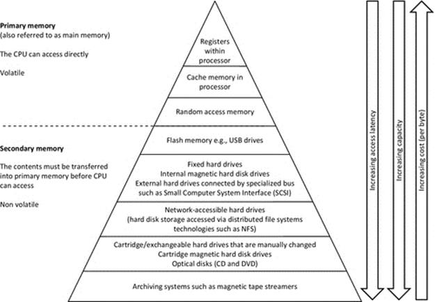
FIGURE 4.7 The memory hierarchy.

RAM is so named because its data locations can be accessed individually, in any order (i.e., we can access memory locations in whatever sequence is necessary as the process runs), and the access order does not affect access time, which is the same for all locations. However, the name can be misleading; there is usually a pattern to the accesses that tends to exhibit spatial or temporal locality. The locations accessed are done so purposefully in a particular sequence and not “randomly.” Spatial locality arises for a number of reasons. Most programs contain loops or even loops within loops, which cycle through relatively small regions of the instruction list and thus repeatedly access the same memory locations. In addition, data are often held in arrays, which are held in a set of contiguous memory locations. Iteration through an array will result in a series of accesses to different, but adjacent, memory locations, which will be in the same memory page (except when a boundary is reached). An event handler will always reference the same portion of memory (where its instructions are located) each time an instance of the event occurs; this is an example of spatial locality, and if the event occurs frequently or with a regular timing pattern, then this is also an example of temporal locality.

The characteristics of secondary storage need to be understood in order to design efficient applications. For example, a hard disk is a block device; therefore, it is important to consider the latency of disk IO in terms of overall process efficiency. It may be more efficient, for example, to read in a whole data file into memory in one go (or at least a batch of records) and access the records as necessary from the cache, rather than reading each one from disk when needed. This is very application-dependent and is an important design consideration.

4.4 Memory Management

In Chapter 2, we looked closely at how the operating system manages processes in the system; in particular, the focus was on scheduling. In this chapter, we examine memory management, which is another very important role of the operating system. There are two main aspects of memory management: dynamic memory allocation to processes (which is covered in depth in a later section) and VM (which is discussed in this section).

As we have seen above, processes use memory to store data, and this includes the contents of messages received from the network or to be sent across the network. Upon creation of a process, the operating system allocates sufficient memory to hold all the statically declared variables; the operating system can determine these requirements as it loads and reads the program. In addition, processes often request allocation of additional memory dynamically; that is, they ask the operating system for more memory as their execution progresses, depending on the actual requirements. Thus, it is not generally possible to know the memory requirements of processes precisely at the time of process creation.

As discussed in the section above, there are several different types of storage in a computer system, and the most common form of primary memory is RAM, which is addressable from the processor directly. A process can access data stored in RAM with low latency, much faster than accessing secondary storage. The optimal situation is therefore to hold all data used by active processes in RAM. However, in all systems, the amount of RAM is physically limited, and very often, the total amount of memory demanded by all the processes in the system exceeds the amount of RAM available.

Deciding how much memory to allocate to each process, actually performing the allocation, and keeping track of which process is using which blocks of memory and which blocks are free to allocate are all part of the memory management role of the operating system. In the earliest systems, once the physical RAM was all allocated, then no more processes could be accommodated. VM was developed to overcome this serious limitation. The simplest way to describe VM is a means of making more memory available to processes than what actually exists in the form of RAM, by using space on the hard disk as temporary storage. The concept of VM was touched upon in Chapter 2 when the suspended process states were discussed. In that chapter, the focus was on the management of processes and the use of the CPU, so we did not get embroiled in the details of what happens when a process' memory image was actually moved from RAM to disk (this is termed being “swapped out”).

Activity R1 explores memory availability and the way this changes dynamically as new memory-hungry processes are created. The activity has been designed to illustrate the need for a VM system in which secondary storage (the hard disk) is used to increase the effective size of primary memory (specifically the RAM).

“Thrashing” is the term used to describe the situation in which the various processes access different memory pages at a high rate, such that the paging system spends almost all of its time swapping pages in and out, instead of actually running processes, and thus, almost no useful work can be performed.

Activity R1

Examine memory availability and use. Observe behavior of system when memory demand suddenly and significantly increases beyond physical availability

Learning Outcomes

1. Understand memory requirements of processes.

2. Understand physical memory as a finite resource.

3. Understand how the operating system uses VM to increase the effective memory availability beyond the amount of physical memory in the system.

This activity is performed in two parts. The first of these involves observing memory usage under normal conditions. The second part is designed to stress-test the VM mechanics of the operating system by suddenly and significantly increasing the amount of memory demanded by processes, beyond the amount of physical RAM available.

Part 1: Investigate memory availability and usage under normal conditions.

Method

(Assume a Windows operating system; the required commands and actions may vary across different versions of the operating system. The experiments were carried out on a computer with Windows 7 Professional installed.)

1. Examine memory availability. Open the Control Panel and select “System and Security,” and from there, select “System.” My computer has 4 GB RAM installed, 3.24 GB usable (available for processes).

2. Use the Task Manager utility to examine processes' memory usage. Start the Task Manager by pressing the Control, Alt, and Delete keys simultaneously and select “Start Task Manager” from the options presented. Select the “Applications” tab to see what applications are running in the system.

3. Select the “Processes” tab, which provides more details than the Applications tab; in particular, it provides memory usage per process. Look at the range of memory allocations for the processes present. These can range from about 50 kB up to hundreds of megabytes. Observe the memory usage of processes associated with applications you are familiar with, such as Windows (File) Explorer and Internet Explorer and perhaps a word processor; are these memory usage values in the ranges that you would have expected? Can you imagine what all that memory is being used for?

4. With the Task Manager “Processes” tab still open for diagnostic purposes, start the Notepad application but do not enter any characters into the form. How much memory is needed for the application itself? We could call this the memory overhead, as this much memory is needed for this application without including any user data (in my system, this was 876 kB). I typed a single character and the memory usage went up to 884 kB; does that tell us anything useful? I don't have access to the source code for this application, but it seems as if a single memory page of 8 kB was dynamically allocated to hold the user data. If I am right, then typing a few more characters will not further increase the memory usage; try it. After some experimentation, I found that Notepad allocates a further 8 kB of memory for approximately each 2000 characters typed into the form. This is approximately what I would expect and is quite efficient; using 4 bytes of memory to hold all the information, it needs about each character of data. You should experiment further with this simple application as it is an accessible way to observe dynamic memory allocation in operation in a real application.

Part 2: Investigate system behavior when memory demand increases beyond the size of physical RAM available in the system.

Caution! This part of the activity can potentially crash your computer or cause data loss. I recommend that you follow this part of the activity as a “pseudo activity,” since I have performed the activity and reported the results so you can observe safely without actually risking your system. The source code for the Memory_Hog program is provided so that you can understand its behavior. If you choose to compile and run the code, make sure you first save all work, close all files, and shut down any applications, which may corrupt data.

Method

(Part 2A uses the system default page file size, which is 3317 MB; this is approximately the same size as the amount of physical RAM installed; the VM size is the sum of the usable RAM plus the page file size and was 6632 MB for this experiment.)

5. Keep the Task Manager “Processes” tab open for diagnostic purposes, while completing the following steps. You can also use the “Performance” tab to inspect the total memory in use and available in the system.

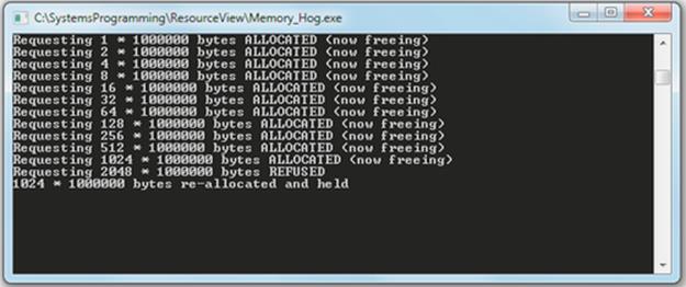
6. Execute a single copy of Memory_Hog within a command window to determine the maximum amount of memory that the operating system will allocate to a single process. The Memory_Hog requests increasing memory amounts, starting with 1 megabyte (MB). Each time it is successful, it frees the memory, doubles the request size, and requests again. This is repeated until the request is refused by the operating system, so the maximum it gets allocated might not be the exact maximum that can be allocated, but it is in the approximate ballpark, and certainly, the system will not allocate twice this much. The screenshot below shows the output of the Memory_Hog on my computer. The maximum size that was successfully allocated was 1024 MB.

7. Execute multiple copies of the Memory_Hog each in a separate command window. Do this progressively, starting one copy at a time and observing the amount of memory allocated to each copy, both in terms of the output reported by the Memory_Hog program and also by looking at the Task Manager “Processes” tab. I used the Task Manager “Performance” tab to inspect the amount of memory committed, as a proportion of the total VM available. The results are presented in the table below.

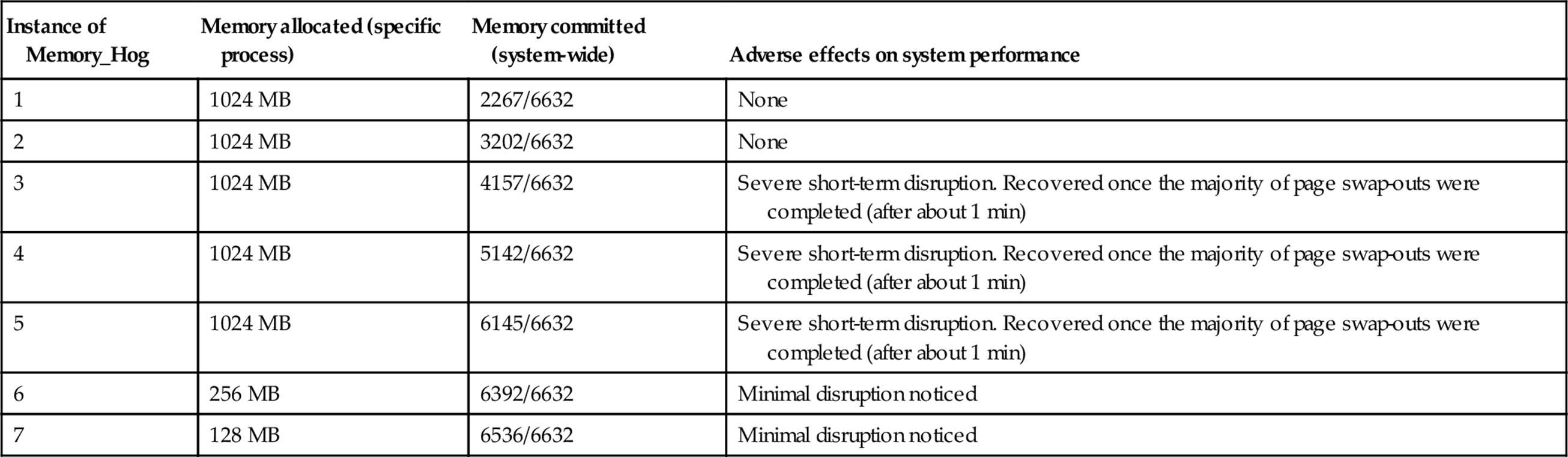
The first and second instances of the Memory_Hog process were allocated the process maximum amount of memory (1024 MB, as discovered in step 6 above). This was allocated without exceeding the amount of physical RAM available, so there was no requirement for the VM system to perform paging.

The third, fourth, and fifth instances of the Memory_Hog process were also allocated the process maximum amount of memory (1024 MB). However, the memory requirement exceeded the physical memory availability, so the VM system had to swap currently used pages out to disk to make room for the new memory allocation. This caused significant disk activity for a limited duration, which translated into system disruption; processes became unresponsive and the media player stopped and started the sound in a jerky fashion (I was playing a music CD at the time). Eventually, the system performance recovered once the majority of the disk activity was completed. No data were lost and no applications crashed, although I had taken the precaution of closing down almost all applications before the experiment.

The sixth instance of the Memory_Hog process was allocated 256 MB of memory. The VM system had to perform further swap-outs, but this was a much smaller proportion of total memory and had a much lower, almost unnoticeable effect on system performance.

The seventh instance of the Memory_Hog process was allocated 128 MB of memory. As with the sixth instance, the VM system performed further page swap-outs, but this had an almost unnoticeable effect on system performance.

When evaluating the system disruption effect of the Memory-Hog processes, it is important to consider the memory-use intensity of the large amounts of memory it requests. If you inspect the source code for the Memory_Hog program, you will see that once it has allocated the memory, it does not access it again; it sits in an infinite loop after the allocation activity, doing nothing. This makes it easy for a paging mechanism based on Least Frequently Used or Least Recently Used memory pages to be able to identify these pages for swapping out. This indeed is the effect witnessed in the experiments and explains why the system disruption is short-lived. If the processes accessed all of their allocated memory aggressively, then the system disruption would be continual, as the paging would be ongoing, for each process. If multiple processes are making such continuous access, then the VM system may begin to “thrash.” This means that the VM system is continually moving pages between memory and disk and that processes perform very little useful work because they spend most of the time in the blocked state waiting for a specific memory page to become available for access.

Method

(Part 2B uses an increased page-file size of 5000 MB, which exceeds the physical memory size significantly. The VM size in this case was 8315 MB.)

8. Execute multiple copies of the Memory_Hog each in a separate command window, progressively as in step 7. The results are presented in the table below.

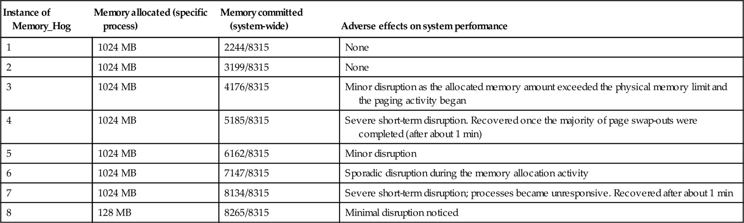
A similar pattern of disruption was observed as with the experiment in part 2A. When the total memory requirement can be satisfied with physical memory, there is no system performance degradation. Once the VM system starts performing page swaps, the performance of all processes is potentially affected. This is due to the latency of the associated disk accesses and the fact that a queue of disk access requests can build up. Once the majority of page swaps necessary to free the required amount of memory for allocation have been completed, the responsiveness of the other processes in the system returns to normal.

Reflection

This activity has looked at several aspects of memory availability, allocation, and usage. The VM system has been investigated in terms of its basic operation and the way in which it extends the amount of memory available beyond the size of physical memory in the system.

When interpreting the results of parts 2A and 2B, it is important to realize that the exact behavior of the VM system will vary each time the experiment is carried out. This is because the sequence of disk accesses will be different each time. The actual set of pages that are allocated to each process will differ as will the exact location of each page at any particular instant (i.e., whether each specific page is held on disk or in physical RAM). Therefore, the results will not be perfectly repeatable, but can be expected to exhibit the same general behavior each time. This is an example of nondeterministic behavior that can arise in systems: It is possible to describe the behavior of a system in general terms, but it is not possible to exactly predict the precise system state or low-level sequence of events.

4.4.1 Virtual Memory

This section provides an overview of the mechanism and operation of VM.

Figure 4.8 illustrates the mapping of process' memory space into the VM system and then into actual locations on storage media. From the process' viewpoint, its memory is a contiguous block, which is accessible on demand. This requires that the VM mechanism is entirely transparent; the process accesses whichever of its pages it needs to, in the required sequence. It will incur delays when a swapped out page is requested, leading to a page fault which the VM mechanism handles, but the process will be moved to the blocked state while this takes place and is unaware of the VM system activity. The process does not need to do anything differently to access the swapped out page, so effectively, the VM mechanism is providing access transparency. The VM system however is aware of the true location of each memory page (which it keeps track of in a special page table), the set of pages that are in use by each process and the reference counts or other statistics for each page (depending on the page replacement algorithm in use). The VM system is responsible for keeping the most needed memory pages in physical memory and swapping in any other accessed pages on demand. The physical memory view reflects the true location of memory pages, which is either the RAM or a special file called the page file on the secondary storage (usually a magnetic hard disk).

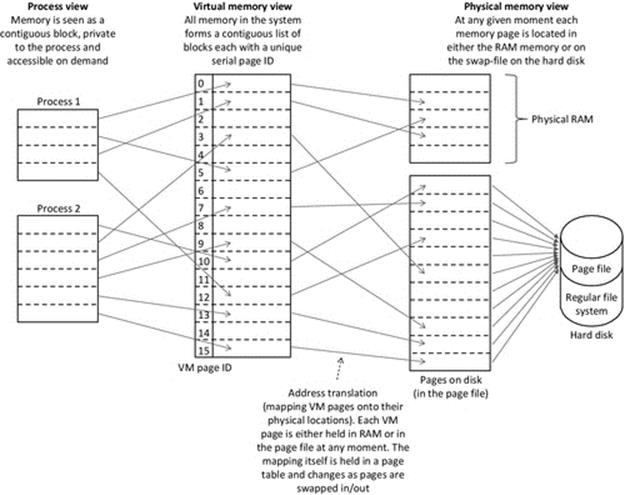
FIGURE 4.8 VM overview.

4.4.1.1 VM Operation

Memory is divided into a number of pages, which can be located either in physical memory or on the hard disk in the page file. Each memory page has a unique VM page number. Memory pages retain their VM page number but can be placed into any numbered physical memory page or disk page slot as necessary.

A process will use one or more memory pages. The memory pages contain the actual program itself (the instructions) and the data used by the program.

The CPU is directly connected to the physical memory via its address and data buses. This means that it can directly access memory contents that are contained in pages that are held in physical memory. All memory pages have a VM page ID, which is permanent and thus can be used to track a page as it is moved between physical memory and the page file on disk.

Memory pages that are not currently held in physical memory cannot be immediately accessed. These have to be moved into the physical memory first and then accessed. Running processes can thus access their in-memory pages with no additional latency but will incur a delay if they need to access a page currently held on disk.

Some key terms are defined:

Swap-out: A VM page is transferred from physical memory to disk.

Swap-in: A VM page is transferred from disk to physical memory.

Page fault: Processes can only access VM memory pages that are held in physical memory. A page fault is the name given to the error that occurs when an attempt is made to access a memory page that is not currently in physical memory. To resolve a page fault, the relevant page must be swapped in. If there are no physical memory pages available to permit the swap-in, then another page must be swapped out first to free space in physical memory.

Allocation error: If the VM system cannot allocate sufficient memory to satisfy a memory allocation request from a process, an allocation error will occur.

Thrashing: When processes allocate a lot of memory, such that a significant amount of the swap file is used and also makes frequent access to the majority of their allocated pages, the VM system will be kept busy swapping out pages to make room for required pages and then swapping in those required pages. This situation is worse when there is low spatial locality in the memory accesses. In extreme cases, the VM system is continuously moving pages between memory and disk, and processes are almost always blocked, waiting for their memory page to become available. The system becomes very inefficient, as it spends almost all of its effort moving pages around and the processes present perform very little useful work.

As is reflected in the results of Activity R1, the overall performance of the VM system depends in part on the size of the swap file allocated on the disk. The swap file size is usually chosen to be in the range of 1-2 times the primary memory size, with 1.5 times being a common choice. It is difficult to find an optimum value for all systems, as the amount of paging activity that occurs is dependent on the actual memory-use behavior of the processes present.

4.4.1.2 Page Replacement Algorithms

When a page in memory needs to be swapped out to free up some physical memory, a page replacement algorithm is used to select which currently in-memory page should be moved to disk.

There are a variety of different page replacement algorithms that can be used. The general goal of these is the same: to remove a page from memory that is not expected to be used soon and store it on the disk (i.e., swap out this page) so that a needed page can be retrieved from disk and placed into the physical memory (i.e., the needed page is swapped in).

4.4.1.3 General Mechanism

As processes execute, they access the various memory pages as necessary, which depends on the actual locations where the used variables are held. Access to a memory location is performed either to read the value or to update the value. If even a single location within a page is accessed, it is said to have been referenced, and this is tracked by setting a special “referenced bit” for the specific page. Similarly, modification of one or more locations in a page is tracked by setting a special “modified bit” for the specific page. The referenced and/or modified bits are used by the various page replacement algorithms to select which page to swap out.

4.4.1.4 Specific Algorithms

The Least Recently Used (LRU) algorithm is designed to keep pages in physical memory that have been recently used. This works on the basis that most processes exhibit spatial locality in their memory referencing behavior (i.e., the same subset of locations tend to be accessed many times over during specific functions, loops, etc.), and thus, it is efficient to keep the pages that have been recently referenced in physical memory. Referenced bits are periodically cleared so that old reference events are forgotten. When a page needs to be swapped out, it is chosen from those that have not been recently referenced.

The Least Frequently Used (LFU) algorithm keeps track of the number of times a VM page in physical memory is referenced. This can be achieved by having a counter (per page) to keep track of the number of references to that page. The algorithm selects the page with the lowest reference count to swap out. A significant issue with LFU is that it does not take into account how the accesses are spread over time. Therefore, a page that was accessed many times, for example, in a loop, a while ago may show up as being more important than a page that is in current use but is not used so repetitively. Because of this issue, the LFU algorithm is not often used in its pure form, but the basic concept of LFU is sometimes used in combination with other techniques.

The First-In, First-Out (FIFO) algorithm maintains a list of the VM pages in physical memory, ordered in terms of when they were placed into the memory. Using a round-robin cycle through the circular list, the algorithm selects the VM page that has been in physical memory the longest, when a swap-out is needed. FIFO is simple and has low overheads but generally performs poorly as its basis for selection of pages does not relate to their usage since they were swapped in.

The clock variant of FIFO works fundamentally in the same round-robin manner as FIFO, but on the first selection of a page for potential swapping out, if the referenced bit is set, the page is given a “second chance” (because at least one access to the page has occurred). The referenced bit is cleared and the round robin continues from the next page in the list until one is found to swap out.

The Random algorithm selects a VM page randomly from those that are resident in physical memory for swapping out. This algorithm is simpler to implement than LRU and LFU because it does not need to track page references. It tends to perform better than FIFO, but less well than LRU, although this is dependent on the actual patterns of memory accesses that occur.

The performance of a page replacement algorithm is dependent on the general memory-access behavior of the mix of processes in the system. There is no single algorithm that works best in all circumstances, in terms of it being able to correctly predict which pages will be needed again soon and thus keep these in physical memory. The various algorithms discussed above have relative strengths and weaknesses, which are highlighted with the aid of some specific scenarios below:

• LRU and LFU are well suited to applications that allocate a large amount of memory and iterate through it or otherwise access it in a predictable way in which there is a pattern to references, for example, a scientific data processing application or a simulation that uses techniques such as computational fluid dynamics (as used, e.g., in weather prediction). In such scenarios, the working set of pages at any moment tends to be a limited subset of the process' entire memory space, so pages that have not been used recently are not particularly likely to be needed in the short term. Depending on the relative size of the working set of pages and the total allocated memory, the clock variant of FIFO may work well.

• An application that has a very large allocated memory and uses the contents very sparsely and with low repetition will have a much less regular patterns in terms of the pages used. In this case, it is very difficult to predict which pages will be needed next and which ones are thus likely to be good candidates to swap out. In such a case, the Random algorithm may perform relatively better than it would with programs that display greater temporal or spatial locality, since no algorithm is able to predict very well, but the Random algorithm at least has very low overheads.

Memory management behavior can be investigated using the Operating Systems Workbench. The VM simulation demonstrates the need for VM and facilitates experimentation with swapping pages between RAM and the hard disk as necessary to meet the applications' memory needs. Activity R2 examines the basics of the VM mechanism and its operation and does not focus on any particular algorithm although the simulation can support evaluation of specific page replacement algorithms, which can be investigated subsequently (see Section 4.11).

Activity R2

Using the Operating Systems Workbench to explore the basics of memory management and VM

Prerequisite: Download the Operating Systems Workbench and the supporting documentation from the book's supplementary materials website. Read the document “Virtual Memory—Activities and Experiments.”

Learning Outcomes

1. To gain an understanding of the need for memory management

2. To gain an understanding of the operation of VM

3. To gain an understanding of the meaning of “page fault,” “swap-out,” and “swap-in”

4. To explore the basics of page replacement algorithms

This activity uses the “virtual memory” simulation provided by the Operating Systems Workbench on the Memory Management tab. The simulation provides an environment in which there are four pages of physical memory and a further eight pages of storage on the disk. Each page holds 16 characters. Either one or two simple text-editing type applications (which are built in to the simulation) can be used to access the memory, for the purpose of investigating the memory management behavior.

Part 1: Simple illustration of the need for, and basic concept of, VM.

Method

1. Enable the first application.

2. Carefully type the letters of the alphabet (from A to Z) in uppercase initially and then repeat in lower case and watch how the characters are stored in the memory as you type. This initial block of text comprises 52 characters. The memory is organized into 16-character pages, so this text spans 4 pages. At this point, all of the text you have typed is held in VM pages currently in physical memory—this is an important observation.

3. Now, type the characters “11223344556677889900”; this adds another 20 characters, totaling 72, but the four physical memory pages can only hold only 64, so what happens? We get a page allocation error.

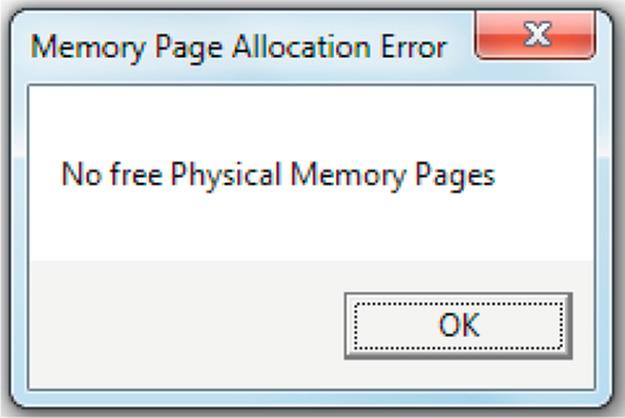
4. You have exhausted the physical memory when you get to the first “7” character. The solution is to select one of the four VM pages in use, to be swapped out (i.e., stored in one of the disk pages), thus freeing up a physical memory page so that you can finish typing your data. Select VM page 0 and press the adjacent “Swap OUT (to Disk)” button. Notice that VM page 0 is moved onto the disk and that the “7” character is now placed into the new page (VM page 4), at the physical page 0 address. Now, you can continue typing the sequence.

The screenshot below shows what you should see after step 4 has been completed.

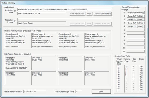
Expected Outcome for Part 1

You can see how your application is using five pages of memory, but the system only has four physical pages. This is the fundamental basis of VM; it allows you to use more memory than you actually have. It does this by temporarily storing the extra pages of memory on the disk, as you can see in the simulation.

Part 2: An example of a page fault; we shall now try to access the memory page that is held on the disk. This part of the activity continues from where part 1 above left off.

5. Try to change the first character you typed, the “A,” into an “@” by editing the application data in the same text box where you originally typed it. You will get a “page fault” because this character is in the page that we swapped out to disk; that is, at present, the process cannot access this page.

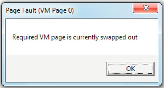
6. We need to swap in VM page 0 so we can access it—press the button labeled “Swap IN (to Memory)” for VM page 0 at the top of the right-hand pane. What happens? We get a page allocation error, because there are no free pages of physical memory that can be used for the swap-in.

7. We need to select a page to swap out so as to create space to swap in VM page 0. Ideally, we will choose a page that we won't need for a long time, but this can be difficult to predict. In this case, we shall choose VM page 1. Press the button labeled “Swap OUT (to Disk)” for VM page 1 at the top of the right-hand pane. Notice that VM page 1 is indeed swapped out and appears in the disk pages section of the display.

8. Now, we try to swap in VM page 0 again. Press the button labeled “Swap IN (to Memory)” for VM page 0 at the top of the right-hand pane again. This time, it works and the page appears back in physical memory—but not in its original place—the contents are still for page 0, but this time, the page is mapped as physical page 1. This is a very important point to note: The system needs to keep a mapping of the ordering of the pages and this is done by the fact that the page is still numbered as VM page 0. The frame table for application 1 confirms that it is using page 0 (as well as pages 1, 2, 3, and 4). Note also that as soon as the page reappears in physical memory, the application is able to access it and the “A” is finally changed to the “@” you typed.

The screenshot below shows what you should see after step 8 has been completed.

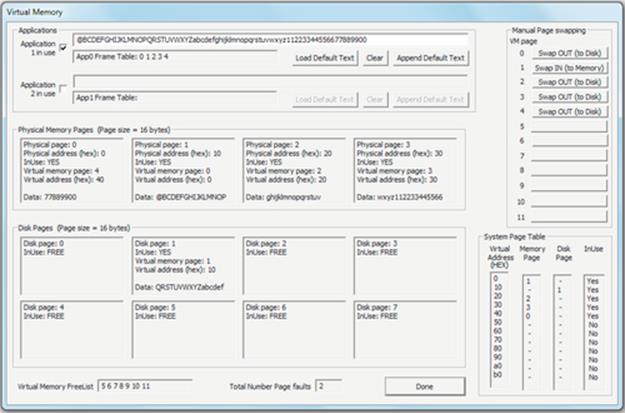
Expected Outcome for Part 2

You should be able to see how the VM pages have been moved between physical memory and disk as necessary to make more storage available than the actual amount of physical memory in the system and to enable the application to access any of the pages when necessary. Note that steps 6-8 were separated for the purpose of exploration of the VM system behavior, but in actual systems, these are carried out automatically by the VM component of the operating system.

Reflection

It is important to realize that in this activity, we have played the role of the operating system by choosing which page to swap out on two occasions: first, to create additional space in the physical memory and, second, to reload a specific swapped out page that we needed to access. In real systems, the operating system must automatically decide which page to swap out. This is achieved using page replacement algorithms that are based on keeping track of page accesses and selecting a page that is not expected to be needed in the short term, on a basis such as it being either the Least Recently Used or Least Frequently Used page.

Further Exploration

VM is one of the more complex functions of operating systems and can be quite difficult to appreciate from a purely theoretical approach. Make sure you understand what has happened in this activity, the VM mechanism by which it was achieved, and the specific challenges that such a mechanism must deal with. Carry out further experiments with the simulation model as necessary to ensure that the concept is clear to you.

Figure 4.9 shows the VM manager behavior as the process makes various memory page requests during Activity R2. Part (a) depicts the first four memory page allocation requests, which are all granted. Part (b) shows that the fifth memory page request causes an allocation error (all RAM is in use). Part (c) shows how VM page 0 is swapped out to free RAM page 0, which is then allocated to the requesting process (as VM page 4); this coincides with the end of part 1 of Activity R2. Part (d) shows that when VM page 0 is subsequently requested by the process, it causes a page fault (the page is not currently in RAM). Part (e) shows the steps required to swap in VM page 0 so that the process can access it. E1: VM page 1 was swapped out (from RAM page 1) to disk page 1 (because initially, VM page 0 occupied disk page 0 so disk page 1 was the next available). This frees RAM page 1. E2: VM page 0 was then swapped in to RAM page 1, so it is accessible by the process. This reflects the state of the system at the end of part 2 of Activity R2.

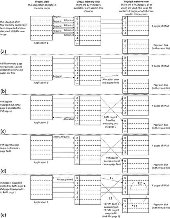
FIGURE 4.9 Illustration of VM manager behavior during Activity R2.

4.5 Resource Management

4.5.1 Static Versus Dynamic Allocation of Private Memory Resources

Memory can be allocated to a process in two ways. Static memory allocation is performed when a process is created, based directly on the declarations of variables in the code. For example, if an array of 20 characters is declared in the code, then a block of 20 bytes will be reserved in the process' memory image and all references to that array will be directed to that 20-byte block. Static memory allocation is inherently safe because by definition, the amount of memory needed does not change as the process is running.

However, there are situations where the developer (i.e., at design time) cannot know precisely how much memory will be needed when a program runs. This typically arises because of the run-time context of the program, which can lead to different behaviors on each execution instance. For example, consider a game application in which the server stores a list of active players' details. Data stored about each player may comprise name, high score, ratio of games lost to games won, etc.; perhaps a total of 200 bytes per player, held in the form of a structure. The designer of this game might wish to allow the server to handle any number of players, without having a fixed limit, so how is the memory allocation performed?

There are two approaches that can be used. One is to imagine the largest possible number of players that could exist, to add a few extra for luck, and then to statically allocate an array to hold this number of player details structures. This approach is unattractive for two reasons: Firstly, a large amount of memory is allocated always, even if only a fraction of it is actually used, and secondly, ultimately, there is still a limit to the number of players that can be supported.

The other approach that is generally more appropriate in this situation is to use dynamic memory allocation. This approach enables an application to request additional memory while the program is running. Most languages have a dynamic memory allocation mechanism, often invoked with an allocation method such as malloc() in C or by using a special operator such as “new” to request that enough memory for a particular object is allocated. Using this approach, it is possible to request exactly the right amount of memory as and when needed. When a specific object that has been allocated memory is no longer needed, the memory can be released back to the available pool. C uses the free() function, while C++ has a “delete” operator for this purpose. In some languages such as C# and Java, the freeing of dynamically allocated memory is performed automatically when the associated object is no longer needed; this is generically termed “garbage collection” (Figure 4.10)

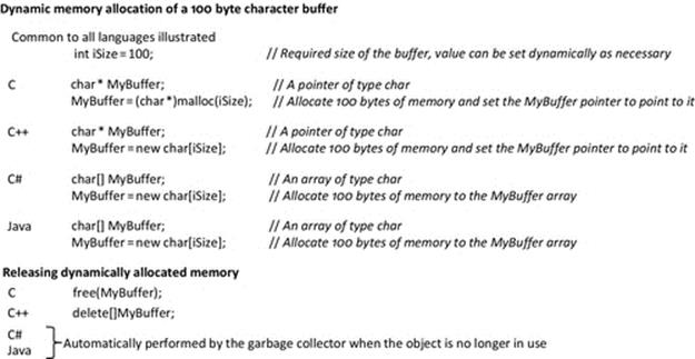
FIGURE 4.10 Dynamic memory allocation of a character array (compare with the static allocation code shown in Figure 4.1).

This approach works very well in applications in which it is easy to identify all of the places in the code and the logical flows through that code, where the objects are created and where the objects need to be destroyed.

However, in programs with complex logic or in which the behavior is dependent on contextual factors leading to many different possible paths through the code, it can be difficult to determine where in the code to allocate and release memory for objects. This can lead to several types of problem, which include the following:

• An object is destroyed prematurely, and subsequently, an access to the object is attempted causing a memory-access violation.

• Objects are dynamically created in a loop that does not terminate properly, thus causing spiraling memory allocation that will ultimately reach the limit that the operating system will allow, leading to an out-of-memory error.

• Objects are created over time, but due to varying paths through the code, some do not get deleted; this leads to an increasing memory usage over time. This is called a “memory leak” as the system gradually “loses” available memory.

These types of problem can be particularly difficult to locate in the code, as they can arise from the run-time sequence of calls to parts of the code which are individually correct; it is the actual sequence of calls to the object creation and object deletion code that is erroneous, and this can be difficult to find with design-time test approaches. These types of problem can ultimately lead to the program crashing after it has been running for some period of time, and the actual behavior at the point of crashing can be different each time, therefore making detection of the cause even harder.

For these reasons, the use of dynamic memory allocation should be treated with utmost respect and care by developers and is perhaps the most important aspect of program design from a memory-resource viewpoint. Figure 4.11 illustrates some common dynamic memory allocation patterns.

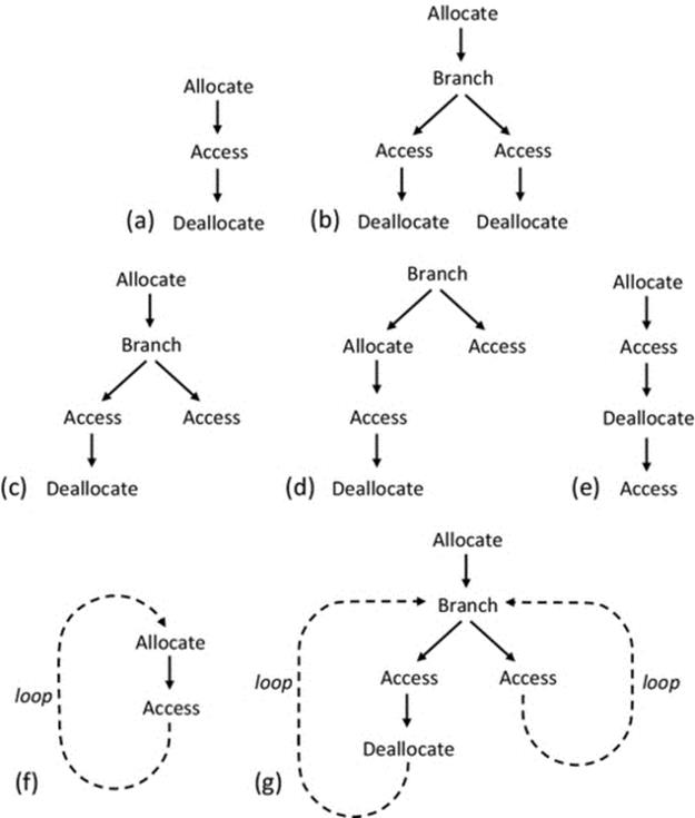
FIGURE 4.11 Dynamic memory allocation and deallocation. Examples of correct sequences and some simplified illustrations of common mistakes.

Common dynamic memory allocation and deallocation sequences are illustrated in Figure 4.11. The scenarios are kept simple for the purpose of clarity and are intended to show general common patterns that arise rather than specific detailed instances. It is clear that if the common mistakes shown can occur in simple cases, there is considerable scope for these problems in larger, complex code with many contextual branches and loops and many function call levels and thus very large numbers of possible logical paths. Therefore, these problems can be very difficult to locate, and it is better to prevent them through high vigilance and rigor in the design and testing stages of development. For the specific patterns shown: (a) is the simplest correct case; (b) illustrates a more complex yet correct scenario; (c) causes a memory leak, but the program logic itself will work; (d) can cause an access violation as it is possible to attempt to access unallocated memory, depending on which branch is followed; (e) causes an access violation because there is an attempt to access memory after it has been de-allocated; (f) causes a behavior to arise that is highly dependent on the loop characteristics—it causes a memory leak, and if the loop runs a large number of times, the program may crash due to memory allocation failure, having exhausted the memory availability limits; (g) is representative of a wide variety of situations with complex logical paths, where some paths follow the allocation and access rules of dynamic memory allocation correctly and some do not. In this specific scenario, one branch through the code de-allocates memory that could be subsequently accessed in another branch. In large software systems, this sort of problem can be very complex to track down, as it can be difficult to replicate a particular fault that may only arise if a certain sequence of branches, function calls, loop iterations, etc. occurs.

4.5.2 Shared Resources

Shared resources must be managed in such a way that the system remains consistent despite several processes reading and updating the resource value. This means that while one process (or thread) is accessing the resource, there must be some restriction on access by other processes (or threads). Note that if all accesses are reads, then there is no problem with consistency because the resource value cannot change. However, even if only some accesses involve writes (i.e., changing the value), then care must be taken to control accesses to maintain consistency.

One way in which a system can become inconsistent is when a process uses an out-of-date value of a variable as the basis of a computation and subsequently writes back a new (but now erroneous) value. The lost update problem describes a way in which this can occur.

Figure 4.12 illustrates the problem of lost updates. The three parts to the figure all represent a scenario in which two threads update a single shared variable. To keep the example simple, one thread just increments the variable's value, and the other thread just decrements the variable's value. Thus, if equal numbers of events occur in each thread, the resulting value should be the same as its starting value. Part (a) shows an ideal situation (that cannot be guaranteed) where two or more processes access a shared resource in an unregulated way without an overlap ever occurring in their access pattern; in such a scenario, the system remains consistent. Part (b) shows how it is possible for the accesses to overlap. In such a case, it is possible that one process overwrites the updates performed by the other process, hence the term “lost update.” In this example, the ADD thread reads the value and adds one to it, but while this is happening, the SUBTRACT thread reads the original value and subtracts one from it. Whichever thread writes its update last overwrites the other thread's update, and the data become inconsistent. In this specific case, one thread adds 1 and one thread subtracts 1, so the value after these two events should be back to where it started. However, you can see that the resulting value is actually one less than it should be. The third event, on the ADD thread, does not actually overlap any other accesses, but the data are already inconsistent before this event starts.

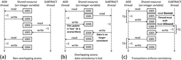
FIGURE 4.12 The problem of lost updates.

To put this “lost update” concept into the context of a distributed application, consider a banking system in which the in-branch computer systems and automatic teller machines (ATM) are all part of a large complex distributed system. The ADD thread could represent someone making a deposit in a branch to a joint account, while at the same time, the SUBTRACT thread represents the other account holder making a withdrawal from an ATM. In an unregulated-access scheme, the two events could overlap as in part (b) of Figure 4.12 depending on the exact timing of the events and the various delays in the system; one of the events could overwrite the effect of the other. This means that either the bank or the account holders lose money!

4.5.3 Transactions

The lost update problem illustrates the need to use special mechanisms to ensure that system resources remain consistent. Transactions are a popular way of achieving this by protecting a group of related accesses to a resource by a particular process from interference arising from accesses by other processes.

The transaction is a mechanism that provides structure to resource access. In overview, it works as follows: When a process requests access to a resource, a check is performed to make sure that the resource is not already engaged in an on-going transaction. If so, the new request must wait. Otherwise, a new transaction is started (preventing access to the resource by other processes). The requesting process then makes one or more accesses that can be read or written in any order, until it is finished with the resource, and the transaction is then terminated and the resource is released.

To ensure that transactions are implemented robustly and provide the appropriate level of protection, there are four criteria that must be met:

Atomicity. The term atomic is used here to imply that transactions must be indivisible. A transaction must be carried out in its entirety, or if any single part of it cannot be completed or fails, then none of it must be completed. If a transaction is in progress and then a situation arises that prevents it from completing, all changes that have been made must be rolled back so that the system is left in the same consistent state as it was originally, before the transaction began.

Consistency. Before a transaction begins, the system is in a certain stable state. The transaction moves the system from one stable state to another. For example, if an amount of money is transferred from one bank account to another, then both the deduction of the sum from one account and the addition of the sum to the other account must be carried out, or if either fails, then neither must be carried out. In this way, money cannot be “created” by the transaction (such as if the addition took place but the deduction did not) or “lost” (such as if the deduction took place but not the addition). In all cases, the total amount of money in the system remains constant.

Isolation. Internally, a transaction may have several stages of computation and may write temporary results (also called “partial” results). For example, consider a “calculate net interest” function in a banking application. The first step might be to add interest at the gross rate (say 5%), so the new balance increases by 5% (this is a partial result, as the transaction is not yet complete). The second step might be to take off the tax due on the interest (say at 20%). The net gain on the account in this particular case should be 4%. Only the final value should be accessible. The partial result, if visible, would lead to errors and inconsistencies in the system. Isolation is the requirement that the partial results are not visible outside of the transaction, so that transactions cannot interfere with one another.

Durability. Once a transaction has completed, the results should be made permanent. This means that the result must be written to nonvolatile secondary storage, such as a file on a hard disk.

These four criteria are collectively referred to as the ACID properties of transactions.

Transactions are revisited in greater depth in Chapter 6 (Section 6.2.4); here, the emphasis is on the need to protect the resource itself rather than the detailed operation of transactions.

Part (c) of Figure 4.12 illustrates how the use of transactions can prevent lost updates and thus ensure consistency. The important difference between part (b) and part (c) of the figure is that (in part (c)) when the ADD thread's activity is wrapped in a transaction T1, the SUBTRACT thread's transaction T2 is forced to wait until T1 has completed. Thus, T2 cannot begin until the shared resource is stable and consistent.

4.5.4 Locks

Fundamentally, a lock is the simple idea of marking a resource as being in-use and thus not available to other processes. Locks are used within transactions but can also be used as a mechanism in their own right. A transaction mechanism places lock activities into a structured scheme that ensures that the resource is first locked, then one or more accesses occur, and then the resource is released.

Locks can apply to read operations, write operations, or read and write operations. Locks must be used carefully as they have the effect of serializing accesses to resources; that is, they inhibit concurrency. A performance problem arises if processes that hold locks on resources do not release them promptly after they finish using the resource. If all accesses are read-only, then the lock is an encumbrance that does not actually have any benefit.

Some applications lock resources at a finer granularity than others. For example, some databases lock an entire table during access by a process, while others lock only the rows of the table being accessed, which enhances concurrency transparency because other processes can access the remainder of the table while the original access activity is ongoing.

Activity R3 explores the need for and behavior of locks and the timing within transactions of when locks are applied and released.

Activity R3

Using the Operating Systems Workbench to explore the need for locks and the timing within transactions of when locks are applied and released

Prerequisite

Download the Operating Systems Workbench and the supporting documentation from the book's supplementary materials website.

Read the document “Threads (Threads and Locks) Activities and Experiments.”

Learning Outcomes

1. To gain an understanding of the concept of a transaction

2. To understand the meaning of “lost update”

3. To explore the need for and effect of locking

4. To explore how an appropriate locking regime prevents lost updates

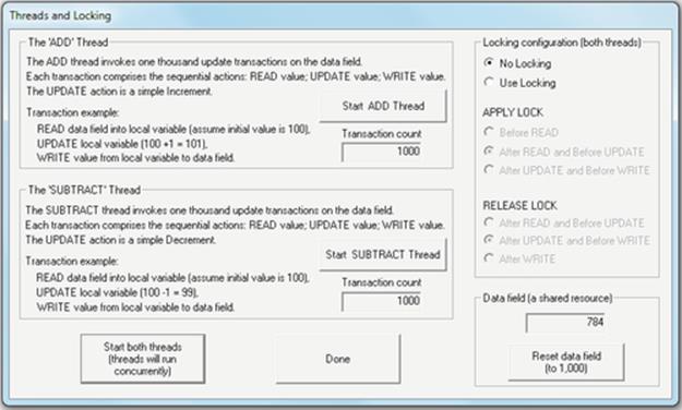
This activity uses the “Threads and Locks” simulation provided by the Operating Systems Workbench. Two threads execute transactions that access a shared memory location.

Part 1: Run threads without locking to see the effect of lost updates.

Method

1. Press the “Reset data field” button and check that the value of the data field is initialized to 1000. Run the ADD thread by clicking the “Start ADD Thread” button. This will carry out 1000 transactions each time adding the value 1. Check if the end result is correct.

2. Now, run the SUBTRACT thread by clicking the “Start SUBTRACT Thread” button. This will carry out 1000 transactions each time subtracting the value 1. Check if the end result is correct (it should be back to the original value prior to step 1).

3. Press the “Reset data field” button again; check that the value of the data field is initialized to 1000. Without setting any locking (leave the selection as “No Locking”), run both threads concurrently by clicking the “Start both threads” button. This will carry out 1000 transactions of each thread. The threads run asynchronously (this concept has been discussed in Chapter 2). Each thread runs as fast as it is allowed, carrying out its particular action (so either adding or subtracting the value 1 from the data value). Check the end result—is it correct?

The screenshot below provides an example of the behavior that occurs when the two threads are run concurrently without locking.

Expected Outcome

Overlapped (unprotected) access to the memory resource has led to lost updates, so that although each thread has carried out the same number of operations (which in this simulation are designed to cancel out), the end result is incorrect (it should be 1000).

Part 2: Using locks to prevent lost updates

Method

Experiment with different lock and release combinations to determine at which stage in the transaction the lock should be applied and at which stage it should be released to achieve correct isolation between transactions and thus prevent lost updates.

1. On the right-hand pane, select “Use Locking.”

2. The transactions in the two threads each have three stages, during which they access the shared data field (Read, Update, and Write). The APPLY LOCK and RELEASE LOCK options refer to the point in the transaction at which the lock is applied and released, respectively. You should experiment with the APPLY and RELEASE options to determine which combination(s) prevents lost updates.

The second screenshot shows a combination of lock timing that results in complete isolation of the two threads' access to the memory resource, thus preventing lost updates.

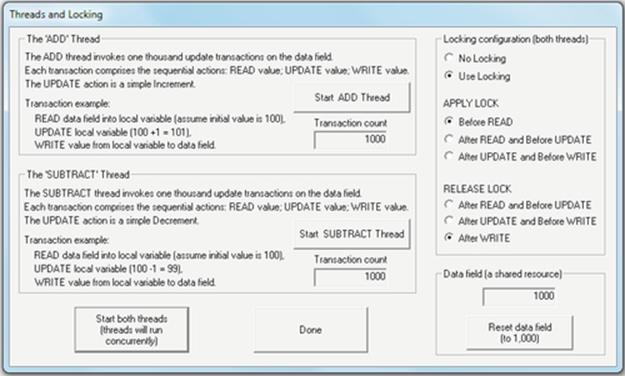
Expected Outcome

Through experimentation with the various lock timing combinations, you should determine that the isolation requirements of transactions are only guaranteed when all accesses to the shared resource are protected by the lock. Even just allowing one thread to read the data variable before the lock is applied is problematic if the second thread then changes the value before releasing the lock so that the first thread can write its change (which is based on the previously read value). See the main text for full discussion of lost updates.

Reflection

This activity has illustrated the need for protection when multiple processes (or threads) access a shared resource. To ensure data consistency, the four ACID properties of transactions must be enforced (see main text for details).

4.5.5 Deadlock

Depending on the way in which resources are allocated and on which resources are already held by other processes, a specific problem called deadlock can arise in which a set of two or more processes are each waiting to use resources held by other processes in the set, and thus, none can proceed. Consider the situation where two processes P1 and P2 each require to use resources R1 and R2 in order to perform a particular computation. Suppose that P1 already holds R1 and requests R2 and that P2 already holds R2 and requests R1. If P1 continues to hold R1 while it waits for R2 and P2 continues to hold R2 while waiting for R1, then a deadlock occurs—that is, neither process can make progress because each requires a resource that the other is holding, and each will continue to hold the resource until it has made progress (i.e., used the resource in its awaited computation). The situation is permanent until one of the processes is removed from the system. Figure 4.13 illustrates this scenario.

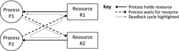
FIGURE 4.13 A deadlock cycle.

For the system shown in Figure 4.13, a deadlock is possible. This is indicated by the fact that the arrows can be followed in a complete cycle. However, this does not mean that a deadlock will actually occur; it depends on the timing and ordering of the various resource requests. Specifically, there are four conditions that must hold simultaneously in order for a deadlock to occur; these are the following:

1. Mutual exclusion. Resources already held by processes are nonshareable; that is, the holding process has exclusive access to them. A process may hold one or more resources in this way.

2. Hold and wait. While holding at least one resource, a process waits for another resource (i.e., it does not release already held resources while waiting).

3. No preemption. Processes cannot be forced to release resources that they are holding; they can be held indefinitely.

4. Circular wait. A cycle is formed of two or more processes, each holding resources needed by the next one in the cycle. For example, Figure 4.13 shows a cycle where process P1 holds a resource R1 needed by process P2, which in turn holds a resource R2 needed by P1; hence, the cycle is complete.

If these four conditions hold, a deadlock occurs. The only way to resolve the situation is to stop (kill) one of the processes, which causes the resources it was holding to be released. Deadlock detection and resolution are additional roles within the resource allocation umbrella that the operating system should ideally perform. It is however the responsibility of application developers to understand the nature of deadlock and thus identify and avoid (to the extent possible) circumstances where it may occur.

Deadlock is explored in Activity R4, using the Deadlock simulation within the Operating Systems Workbench.

The occurrence of deadlock is sensitive to the relative timing of events, and there is usually a limited window of opportunity where a deadlock will actually occur, as the resource acquisition stages of transactions have to relate to the same set of resources and overlap in time. Identifying that a deadlock may occur does not actually mean that a deadlock will occur. The theoretical technique of cycle drawing is used to determine if a deadlock is possible, but this does not indicate actual probability of deadlock. The deadlock simulation allows exploration of the factors that affect the likelihood of a deadlock.

The deadlock simulation characteristics are described below. Note that the simulation user interface refers to threads, so the discussion below does for consistency. However, the deadlock simulation equally applies at the level of processes within a system, as it does at the level of threads within a process.

• The number of resources per transaction is one or more and chosen randomly up to the limit number that each thread is permitted to use (but also within the limit number of resources enabled in the simulation).

• The actual resources to be used in a particular transaction are chosen randomly from the set that is enabled.

• The resources are considered shared, so each thread makes its decision to use a resource independently of what the other thread is doing and what resources it is using.

• Threads acquire resources individually and lock them while waiting to acquire others (the hold and wait condition).

• Once all resources needed are held, the transaction begins. There is no preemption; held resources are only released at the end of the transaction.

• A resource is used exclusively by the thread that holds it.

• A circular wait develops if a thread is waiting for a resource held by another thread, which is itself waiting for a resource held by another thread in the same chain, such that a complete cycle forms. This is easy to see in the simulation because only two threads will be involved. In real systems, it is possible for cycles to involve more than two threads, and these of course can be complex in nature and difficult to detect.

Activity R4

Using the Operating Systems Workbench to explore deadlock during resource allocation

Prerequisite: Download the Operating Systems Workbench and the supporting documentation from the book's supplementary materials website.

Read the document “Deadlock—Activities and Experiments.”

Learning Outcomes

1. To gain an understanding of the nature of deadlock

2. To explore the circumstances required for deadlock to occur

3. To explore factors that affect the likelihood of a deadlock

This activity uses the “Deadlock” simulation provided by the Operating Systems Workbench. Up to two threads are supported (the simulation applies conceptually to either threads or processes), which compete for up to 5 resources.

Part 1: Exploration of the nature of deadlock and the conditions under which it can occur

Method

1. Run the simulation with a single thread by clicking the top leftmost button entitled “Start Thread.” Experiment with different numbers of resources, by enabling or disabling them with the column of buttons to the right of center. Using the radio buttons at top right, set the maximum number of resources each thread is permitted to use to 2. Does deadlock occur? Do your observations indicate that a deadlock can occur in these circumstances?

2. Repeat step 1 but this time using both threads and only a single resource. Does deadlock occur in this case?

3. Repeat step 1 again, now using both threads and two resources. Does deadlock occur in this case?

The screenshot below from step 3 of part 1 shows the situation when a deadlock has occurred.

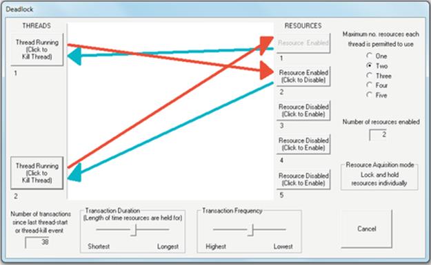
Expected Outcome

A deadlock is detected by having a cycle in the resource allocation pattern. This is seen in the screenshot. You can see that thread 1 has acquired resource 1 (blue arrow) and is waiting for resource 2 (red arrow). At the same time, thread 2 has acquired resource 2 and is waiting for resource 1. The arrows form a directed cycle (i.e., the arrows all point in the same direction around the cycle). The only way to break this cycle is to kill one of the threads; this will cause the held resource to be released and thus the remaining thread will be granted access to it and can continue with its transaction.

Part 2: Exploration of factors that affect the likelihood of deadlock

In this part of the activity, you should explore different configurations of the simulation and observe how this affects the likelihood of deadlock. Use both threads for this part of the experiment. Initially change only one parameter at a time, as set out in the four steps below. Once you think you understand the circumstances that make deadlocks more or less likely, then try changing several parameters at the same time to confirm or reinforce your understanding.

1. Experiment with different numbers of resources available (enabled) for the two threads to use.

2. Experiment with different limits on the number of resources each thread is permitted to use simultaneously.

3. Experiment with different values of the transaction duration.

4. Experiment with different values of transaction frequency.

The screenshot below relates to part 2. It shows a scenario with five resources active but each process only using a maximum of two.

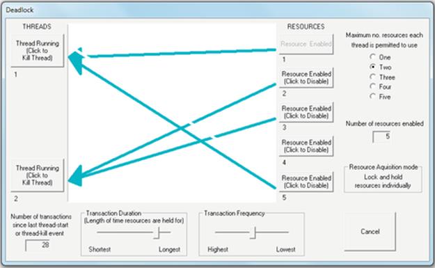
Expected Outcome

In part 2 of the activity, you should see that deadlock likelihood is affected by certain factors. For example, the longer a resource is held while acquiring others (use the “transaction duration” control to adjust this), the greater the window of opportunity for deadlock. The more resources a thread uses, the greater the opportunity for deadlock, while having more resources available for use dilutes the probability that the threads will each use the same set of resources (see the screenshot above as an example where two threads simultaneously use two resources each without conflict).

Reflection

Deadlock prevents threads continuing with their work and thus impacts on the performance of specific tasks and also on the robustness of systems themselves because deadlock resolution involves killing one of the threads that may then have to be restarted, depending on circumstances. Realization of the way in which deadlock can occur and the factors that affect its likelihood is important for the design of robust and efficient distributed systems.

Further exploration

Carry out further experiments with the deadlock simulation until you have a clear appreciation of the cause of deadlock and the factors, which increase its likelihood of occurrence.

4.5.6 Replication of Resources

This section introduces the concept of replication of resources as it is important as part of the resource view of systems. Chapter 5 discusses replication in greater detail, including the semantics of replication, and provides an activity in which an example implementation of replication is explored. In addition, replication transparency is discussed in Chapter 6.

Having only a single copy of each resource in a distributed system is limiting in several ways. A key issue is the possibility of permanent loss of data. There is a risk that the resource will be lost; for example, if stored on a single hard disk, it is susceptible to a disk crash or physical damage to the host computer caused by fire or flood, for example, or even theft of the computer. If the only up-to-date copy of a resource is held temporarily in volatile memory such as RAM, it is susceptible to the computer being switched off or a momentary interruption to the power supply.

There is also a risk that shared access to a specific resource will become a performance bottleneck and may limit the usability or scalability of the system. For example, if the resource in question is a highly visited web page hosted on a single server, then the accessibility of the web page is limited by the processing throughput of the computer on which the server sits and also limited by the throughput of the network and of the connection to the computer. These limitations translate into a cap on the number of simultaneous users who can access the resource with an acceptable response time.

A further risk arises in terms of availability. If there is only a single copy of a specific resource, then its availability is dependent on every component in the chain of access working correctly simultaneously. If the computer on which the resource is hosted has an uptime of 98% (i.e., 2% of the time, it is unavailable because of system maintenance or failures) and the network connection to that computer has a reliability of 99%, then the resource is available for 97.02% of the time. That is, the entire chain of access has a reliability of 0.98 × 0.99 = 0.9702.

To overcome these limitations, it is common to replicate resources in distributed systems. This essentially means that there are multiple copies of the resource stored in different places within the system, thus enhancing robustness, availability, and access latency. The actual number of replicas and their dispersal within a system are system-specific issues that are highly dependent on the particular applications that use the resources. Managers of large commercial distributed applications such as banking, stock trading, and ecommerce will likely choose to ensure that the replicas are spread across multiple geographically spread sites to ensure disaster resilience (protection against such things as natural disasters, civil disturbance, and terrorism). Smaller-scale applications or applications owned by smaller organizations may hold replicas at the same site; but the system architecture should be designed to ensure that they are not on the same physical disk or host computer. The number of replicas should take account of the expected access rate, which in turn is related to the number of concurrent users expected.

The provision of replicas introduces two new main challenges. The first of these is consistency. Each copy of the resource must hold the same value. When one copy is updated, so too must all the other copies be. An application reading one copy of the resource should get the same value as if it were to read any other copy. Data consistency is in itself a major challenge in large-scale distributed systems, especially if multiple replicas can be write-accessed by applications and have their values changed simultaneously. To limit the extent of this challenge, it is possible to arrange that only one replica at any time can be written to, and all other copies support only read-only access. In this case, the problem is reduced to the need for timely propagation of value updates, from the read-write copy to the read-only copies.

The second main challenge introduced by replication is a special case of transparency requirements. Applications should be designed such that they access a (from their viewpoint) nonreplicated resource, for example, opening a file or updating a database. That is, the host system must provide the illusion of a single instance of the resource, regardless of whether it is replicated or not. The application behavior and its interface to the underlying system must not change because of the replication of one of the resources it uses. Instead, the replication must be managed within the (distributed) system. This form of transparency is termed replication transparency. Lack of this transparency would imply that the application had to be aware of the number of and location of replicas and to update each one directly.

The application developer should not need to be aware of replication; there should be no special actions required because a resource is replicated and no new primitives to use. The application developer should not know (or need to know) that a resource is replicated, how many replica instances exist, where they are located, or what the consistency management mechanism is.

Similarly, users of applications should not be aware of resource replication. A user should have the illusion that there is a single copy of each resource that is robustly maintained and always up-to-date. All details of how this is achieved should be completely hidden.

Consider, for example, your bank account value, which you quite likely access through an Internet online facility. You see a single value of your account balance, which should always be consistent, reflecting accurately the various financial transactions that have been carried out. The fact that in reality, the bank stores your bank account balance value on several computers, likely spread geographically, possibly even internationally, should be of no concern to you. The bank will have in place mechanisms to propagate updates so that replicas remain consistent and to manage recovery if one copy becomes corrupted or inaccessible, using the values of the other copies.

The need for timely propagation of updates to all replicas can be illustrated using the documents that contain the text for this book as a simple example. As I write, I keep copies of the document files on two different hard disks to avoid problems arising from a hardware fault on my computer and from accidental deletion by myself. There are always two copies of the work. In order for this to be effective, I use the copies on one specific drive as the working set and back up the files to the other disk on a regular basis, typically at the end of each couple-of-hour period that I have been working on the book. There are thus moments when the two copies are actually different and there is a risk of losing some work. In this situation, the update rate is chosen to reflect the risk involved. I can accept the risk of losing at most a couple of hours of work. Notice that the lost update problem also applies here. During moments when the copies are unsynchronized, if I accidentally open the older copy, add new material, and then save as the latest version, I will have overwritten some changes I had previously made.

4.6 The Network as a Resource

4.6.1 Network Bandwidth

Bandwidth is the theoretical maximum transmission rate for a specific network technology and thus applies separately to each link in the network depending on which technology is involved. For example, Fast Ethernet has a bandwidth of 100 megabits per second. Bit time is the time taken to transmit a single bit. For any given technology, this value is a constant and is derived as the reciprocal of bandwidth. The bit time for Fast Ethernet is thus 10 ns (or 10^{− 8} s). Throughput is the term used to describe the actual amount of data transmitted.

Network bandwidth will always be finite in a given system. Advances in technology means that over time, bit rates are increasing (so newer technologies support transmitting more data in a given amount of time) and infrastructure is becoming more reliable. However, improvements in network technology can barely keep up with the increasing demands from users to transmit ever more data.

Developments in other technologies also can lead to large increases in network traffic volumes; consider, for example, the improvements in digital camera technology in recent years. Image fidelity has improved from typically 1 megapixel (one million pixels per image) to cameras that produce images of 20 megapixels and more. The actual size of image files produced depends on the image coding and the data compression techniques used. The “True Color” encoding scheme uses 24 bits per pixel; 8 bits are used to represent each of the red, green, and blue components, providing 256 intensity values for each. Thus, before compression, some systems encode 3 bytes of data per pixel in the image. For a 20-megapixel image, this would give rise to a precompression file size of 60 MB. A very popular example of digital image compression is the Joint Photographic Experts Group (JPEG) scheme, which can achieve a compression factor of about 10:1 without noticeable degradation of image quality. Using JPEG, our 20-megapixel image is now reduced to 6 MB, which is still a significant amount of data to be transmitted across a network.

These devices are also increasingly abundant, a high-resolution digital camera is now cheap enough for many people to buy, and of course, other devices such as mobile phones and tablets contain cameras. The situation is further exacerbated by the fact that social networking has become extremely popular in the last couple of years and many people are continually uploading not only large amounts of data in the form of pictures but also other digital media such as sound and video that can represent much larger transfers than still images.¹ On top of all this, the total number of users and the proportion of their daily activities that involve “online” behavior of some sort or another are also increasing rapidly.

We can conclude from the trends in device technology to generate ever-larger data volumes and the trends in society to be ever more dependent on data communication that bandwidth will always be a precious resource that must be used efficiently. A large proportion of network performance problems are related to network bandwidth limitations. Bandwidth is typically shared among many traffic flows, so when we compute the time taken to transfer a certain amount of data over a particular network, based on the bandwidth of a specific link, we must keep in mind that we are calculating the best-case time. For example, if we wish to transmit a file of 100 MB over a 100 megabit per second link, we do the following sum:

So 8 s is the time required to transmit the file at the maximum possible rate, which assumes dedicated access to the link. The actual time to transfer the file depends on the actual share of the link that our application flow uses. In a busy network, the link the file may take considerably longer to transmit over the same link.

The situation is more complex when traversing a path through a network, which comprises several links that may have different bandwidths. In this case, the highest theoretical throughput end-to-end is limited by the slowest link bandwidth on the path.

Designers of distributed applications can never afford to be complacent with respect to the way they use bandwidth. For the reasons explained above, it is not realistic to assume that technological improvements over time (e.g., link speeds will be higher or routers will have faster forwarding rates) will lead to overall better performance as perceived by the users of any particular application.

There are several ways in which an application developer can ensure that their application is efficient with respect to network bandwidth, these fall into two categories: Firstly, minimize what is sent such that only essential communication takes place and, secondly, minimize the overheads of communication through careful selection and tuning of communication protocols.

4.6.1.1 Minimal Transmissions

In order to use network bandwidth effectively and to ensure that individual applications are efficient in their communication behavior, it is important that messages are kept as short as possible. Care should be taken when designing distributed applications to avoid transmission of redundant or unnecessary information. Only the minimum data fields necessary for correct operation should be transmitted; this may require having a number of different message structures for different scenarios within an application, especially where the range of message sizes varies greatly in the same application. The data fields themselves should be as small as possible to contain the necessary information. Messages should only be transmitted when needed and where periodic transmission is necessary; the rate of message transmission should be carefully optimized as a trade-off between timeliness of information update and communication efficiency. In some applications, it might be possible to perform aggregation of several messages at the sending side and transmit the resulting information at a significantly reduced rate. This is particularly relevant for sensor systems where data from sensors are often transmitted periodically. The rate of transmission needs to be aligned to the rate at which the actual sensed attribute changes. For example, the temperature in a residential room or office does not change significantly over a one second period but might do over a 1 min period. Thus, it might be appropriate to send update messages at 1 min intervals, especially if the data are used to control an air conditioning system. If, however, the purpose of measuring temperature is only for historical logging purposes, then it may be better to collect temperature samples every 1 min and aggregate the values of perhaps ten samples together into a single message that is sent every 10 min. The aggregation could be in the form of taking a single average value or by collecting the ten samples into a data array and sending them in a single message (note that in this latter case, the same amount of data is sent, but the amount of communication overhead is reduced). In contrast, if temperature is being sensed within a stage of a chemical process in a production facility, it may be necessary to sample temperate at high rates, perhaps at intervals of 100 ms. In such a scenario, the data may be safety related; it may indicate that a particular valve needs to be closed to prevent a dangerous situation developing. If this is the case, it is necessary to transmit each message immediately in its raw form.

4.6.1.2 Frame Size (Layer 2 Transmission)

Transmission errors (caused by electromagnetic interference, voltage glitches, and cross talk between conductors) impact at the level of individual bits. The probability of a single bit being corrupted by such errors is considered the same for all bits transmitted on a particular link, although some sources of interference occur in bursts and may affect several bits transmitted in a short time frame.

Short frames are less likely to be impacted by bit errors² than longer frames. This is because for a given bit error rate on a link, the probability of the error affecting a particular frame is directly proportional to the size of the frame.

For example, if the bit error rate is 10^{− 6}, one bit error occurs, on average, every 1 million bits transmitted. For a frame of size 10³ bits, the probability of suffering a bit error is 10³/10⁶ = 10^{− 3}, so there is a 1 in 1000 chance that a specific frame will be corrupted. The problem of a corrupted frame is resolved by retransmitting the entire frame; thus, the cost of each bit error is actually 1000 bits of transmission, and so, the overall cost of bit errors for this configuration is 1/1000th of the total resource. However, if the frame size is 10 times larger, fewer frames are sent per second, but the total number of bits transmitted is the same. In this case, the probability of a frame suffering a bit error is 10⁴/10⁶ = 10^{− 2}, so there is a 1 in 100 chance that a specific frame will be corrupted. Retransmitting the frame in this case costs 10,000 bits of transmission. The overall cost of bit errors for this configuration is thus 1/100th of the total resource.

The way in which a particular packet is divided into frames for transmission over a link carries an efficiency trade-off because each frame has a transmission overhead. Using fewer, larger frames translates into lower total overheads (in the absence of errors); however, smaller frames are cheaper to retransmit if affected by a bit error. Figure 4.14 illustrates this efficiency trade-off with an example based on Ethernet.

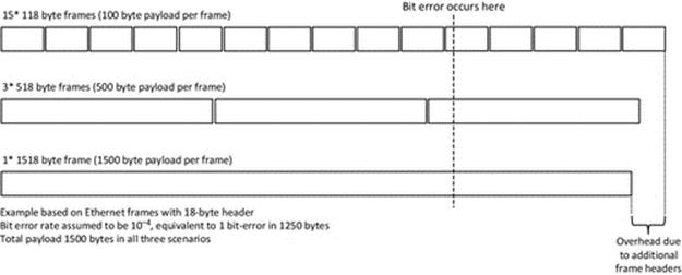
FIGURE 4.14 Frame size relationship with bit error rates.

Figure 4.14 shows three scenarios for transmitting a 1500-byte (12,000 bit) payload over an Ethernet network in terms of the way it is divided into frames. The payload is the maximum size for a single Ethernet frame, and hence, one of the scenarios uses a single, maximum length frame. The other scenarios shown arise from dividing the payload into three and fifteen parts. The frame overhead (the Ethernet header) is 18 bytes. The figure shows the effect of the additional overhead when transmitting the same payload distributed over a higher number of smaller frames. Bit errors operate at the physical level and do not respect frame boundaries; that is, a bit error corrupts the current bit in transmission, regardless of which frame it belongs to. In the example, the bit error rate for the link is assumed to be 10^{− 4}, which means that one bit error occurs on average for every 10,000 bits transmitted (this bit error rate value is used for the purpose of illustration; it would typically be much lower). The payload in this case is greater than 10,000 bits, so there is a high probability that a bit error will occur during its transmission. For the purpose of the example, a bit error is assumed to occur at the same bit position measured from the start of the first transmission, in all three scenarios. The frame that is in transmission when the bit error occurs becomes corrupted and must be retransmitted. Assuming that the retransmissions succeed with no further bit errors, then the true cost of the single bit error is an overhead of 100%, 33%, and 6.7% for the 1518-byte, 518-byte, and 118-byte frame size scenarios, respectively.

The susceptibility of larger frames to bit errors is one of the reasons why link technologies have upper limits on frame sizes; this tends to be in the region of a few hundred to a few thousand bytes. Shorter frames also have advantages in terms of achieving finer-grained multiplexing, thus enhancing the illusion of a dedicated circuit on shared links.

4.6.1.3 Packet Size (Layer 3 Transmission)

From a message transmission viewpoint, packets can be considered as an intermediary format mapping the content of an application-level message into frames. This is because during the encapsulation down, the protocol stack a message is divided into one or more packets, which are each then divided into one or more frames.

Each link in a network has a fixed maximum frame size and thus a maximum payload size within those frames. For a given specific link, the maximum transmission unit (MTU) determines the maximum size of packet that can be carried within a frame. This may be configured at routers up to the maximum frame payload size for the relevant link technology. For example, for Ethernet, the maximum MTU size is 1500 bytes.

With IPv4, packets are fragmented as necessary to fit within the MTU for each link and may get further fragmented by routers as they travel across the network. In IPv6, the sending node is required to determine the MTU for the entire end-to-end journey and to perform the fragmentation based on the determined MTU, such that no further fragmentation is necessary by intermediate routers.

Fragmentation is generally undesirable. Each packet has its own network-layer header, which contains, among other things, the IP address of the destination node that routers use to make packet-forwarding decisions. Each fragment of a packet must contain a modified copy of the original packet header, which indicates the original packet ID to which the fragment belongs and the offset of the fragment within the original packet (for reassembly purposes). Therefore, packet fragmentation and the subsequent reassembly introduce computational overhead at the involved devices. The reassembly process must wait for all fragments to arrive and thus can add latency to the delivery of the packet to the application. A set of smaller packets that avoid fragmentation is potentially more efficient than the equivalent number of fragments derived from a single larger packet.

4.6.1.4 Message Size (Upper Layers Transmission)

Careful design of distributed applications needs to include resource efficiency in terms of network bandwidth, which in turn improves scalability and performance transparency. This of course must be done such that the application's business logic requirements, and any timing constraints, are not affected.

A golden rule for network message design is “only send what is necessary.” The communication design should in general aim to minimize message size. This ensures that the message is transmitted in less time, uses less resource, and contributes less to congestion. Large messages are divided into multiple packets, which are themselves spread across multiple frames, depending on their size. Each frame introduces additional overhead because it must have its own header containing MAC addresses and identification of the next higher-layer protocol. Similarly, each packet introduces additional overhead in terms of its header, which contains IP addresses and identification of the transport layer protocol.

It is important to realize that the effect of reducing message size is not linear in terms of the reduction in number of bits transmitted. Frames have a certain minimum size and some fixed overheads. A message that is increased in size by a single byte could lead to an additional frame being transmitted, while reduction by a single byte could actually save an entire frame. The Ethernet family of technologies is the most popular wired access-network technology and will be used to illustrate this point. To recap, Ethernet has a minimum frame size of 64 bytes, comprising an 18-byte header and a payload of 46 bytes. It also has a maximum frame size of 1518 bytes, in which case the payload is 1500 bytes.

If the message to be sent leads to a frame size of less than the 64-byte minimum, the additional bytes are padded. If we send a TCP protocol message (which typically has a 20-byte header), encapsulated in an IPv4 packet (typically a 20-byte header), then there is room for 6 bytes of data while still keeping within the minimum frame size. There are a few scenarios where this could be achieved, for example, where the message contains data from a single sensor, for example, a 16-bit temperature value, or is an acknowledgment of a previous message that contains no actual data. However, this accounts for a small fraction of all messages within distributed applications; in most cases, the minimum frame size will be exceeded. However, due to the variable payload size up to 1500 bytes, there are a large number of application scenarios where the message would fit into a single Ethernet frame.

The ideal situation would be where the application-level message is divided into a number of packets that each fit within the minimum frame MTU for the entire end-to-end route to their destination, thus avoiding packet fragmentation.

A developer cannot at design time know the link technologies that will be in place when the program actually runs. Therefore, the designer of a distributed application should always try to minimize the size of messages, with the general goal of making the network transmission more efficient but without certainty or precise control of this outcome.

In some applications, there may be choice as to whether to send a series of smaller messages or to aggregate and send a single longer message. There are trade-offs: shorter individual messages are better for responsiveness as they can be sent as soon as they are available, without additional latency. Combining the contents of smaller messages into a single larger message can translate into fewer actual frames, and thus, less bytes are actually transmitted.

Minimizing message size requires careful analysis of what data items are included in the message and how they are encoded. A specific scenario is used to illustrate this: consider an eCommerce application that includes in a query “Customer Age” represented as an integer value. When this is marshaled into the message buffer, it will take up 4 bytes (typically, this aspect depends somewhat on the actual language and platform involved). However, some simple analysis is warranted here. Customer age will be never higher than 255, and thus, the field could be encoded as a single byte or character (char) data type, thus saving 3 bytes. If “Sex” is encoded as a string, it will require 6 characters so that it can hold the values “Male” or Female”; this could be reduced to a single byte if a Boolean value or a character field containing just M or F is used. I would suggest that we can go one step further here, if we consider that customer age cannot for all intents and purposes exceed 127; we can encode it as a 7-bit value and use the single remaining bit of the byte to signify male or female. This is just a simple illustration of how careful design of message content can reduce message sizes, without incurring noticeable computational overheads or complex compression algorithms. Of course, these can be used as well; however, if the data format has already been (near) optimized to maximize information efficiency, the compression algorithms will have a greatly reduced benefit (because they actually work by removing redundancy, which is already reduced by the simple techniques mentioned above). Figure 4.15 illustrates some simple techniques to minimize the size of the message to be transmitted across the network including, for the example given above, a simple and efficient algorithm to perform the encoding.

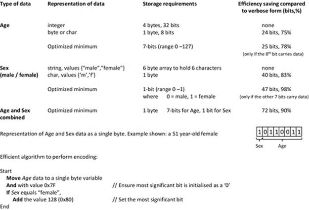
FIGURE 4.15 Examples of simple techniques to minimize data transmission length.

4.6.2 Data Compression Techniques

To minimize network traffic generation by distributed applications, data compression should be considered where appropriate. This is only useful where there is sufficient redundancy in the transmitted data such that the saving in bandwidth is worth the additional processing cost associated with running the data compression and decompression algorithms and where the computer systems have sufficient processing power to perform the data compression suitably quickly.

The technique described in the section above compresses data on a context-aware basis and thus is highly application-specific and is performed as part of the designed-in behavior of the application itself. This is a very useful technique where opportunities present themselves to designers without making the design overcomplex.

There are also data compression techniques that are algorithmic and are applied to the data stream itself. Such algorithms target inefficiencies in coding schemes, reducing the transmitted data size by removing redundancy. The advantage of these techniques is that they do not require additional work on the part of the designer, although they do incur run-time overheads in terms of processing time. However, for most modern computer systems, the processing speed is significantly faster than network transmission speeds, and thus, compression has a net performance benefit as a result of the trade-off between processing time expended and the network latency saved. It is also important to minimize data transmissions to reduce network congestion.

4.6.2.1 Lossy Versus Lossless Compression

There are two fundamental classes of data compression technique: those that lose data and those that do not.

Lossy data compression removes some actual data but leaves enough remaining data for the compressed format to be still usable; however, it is not reversible. A classic example is the reduction of the resolution of an image. The lower-resolution image is still recognizable as the same picture, and thus, the data loss is a useful trade-off between image quality and file size.

An important example of where picture quality reduction is desirable is where they are displayed on web pages. The time taken to download images is directly related to the size of the image file. If the purpose of the transfer is only to display on the screen, then there is no point in transmitting an image that has greater resolution than the display screen itself. In general, a 12-megapixel image will not look any different to a 1-megapixel image when displayed on a screen with a resolution of 1 million pixels (which is equivalent to a grid of, e.g., 1000 pixels by 1000 pixels). However, the 12-megapixel version of the file would take a lot longer to download and contribute much more to the level of traffic on the network.

Actual data, such as financial data or text in a document, cannot be subjected to lossy data compression. It would be meaningless to just remove a few characters from each page of a document to reduce the file size, for example. Instead, lossless techniques must be used. The application-specific example in the section above is a simple form of lossless compression, as the information content is squeezed into a more efficient form of encoding, but with no loss of precision or accuracy.

4.6.2.2 Lossless Data Compression

Huffman coding provides an easy to understand example of lossless data compression. This technique uses a variable length code to represent the symbols contained in the data. It is necessary to perform a frequency analysis on the data to order the symbols in terms of their frequency of occurrence. The shorter code words are assigned to the symbols that occur more frequently in the data stream, and the longer code words are assigned to rarely occurring symbols. This could be performed for a single document or more generally for all documents written in a particular language.

For example, let us consider the English language. The most commonly occurring letters are E, T, A, and O, followed by I, N, S, R, and H, and then D, L, U, C, M, W, F, P, G, Y, and B. The infrequent letters are V, K, and J, and the rarest are X, Q, and Z. Based on this frequency analysis, we can expect that there will be more “E's,” “T's,” “A's” and “O's” (and thus, these should be allocated shorter codes) and few “Q's” and “Z's” (so these should be allocated longer code words).

The code words themselves must be carefully chosen. Since they are of variable length, once a string of code words has been compiled, there must be a way to decode the string back to its original symbols unambiguously. This requires that the receiving process knows the boundaries between the code words in the stream. Sending additional information to demark the boundaries between the code words would defeat the object of compression to minimize the amount of data transmitted, so the code words must be self-delimiting in terms of the boundaries.

To satisfy this requirement, the set of code words used in Huffman coding must have a special prefix property, which means that no word in the code is a prefix of any other word in the code. Without this requirement, when reading a particular code word, it would not be possible to know where the word ended; you could just keep reading into the next word without knowing. For example, if the word 101 was part of the code, then 1011 or in fact any other word beginning with 101 is not allowed. In the example given, the prefix rule would be broken because the code 101 would be a prefix of the code 1011.

A valid code set that exhibits the prefix property can be generated by using a binary tree, in which only leaf nodes are used as codes and nonleaf nodes are used to generate deeper layers of the tree. The tree is extensible to generate additional codes so long as some leafs remain unused for codes at each level. To limit the size of the tree for illustration purposes, imagine that we only need to represent the 26 letters of the alphabet plus the space character and a full stop; that is, we need a total of 28 codes. One way to achieve this is to use the binary tree shown in Figure 4.16 (this particular tree is not necessarily optimal; it is used only to illustrate the generation of a valid code set).

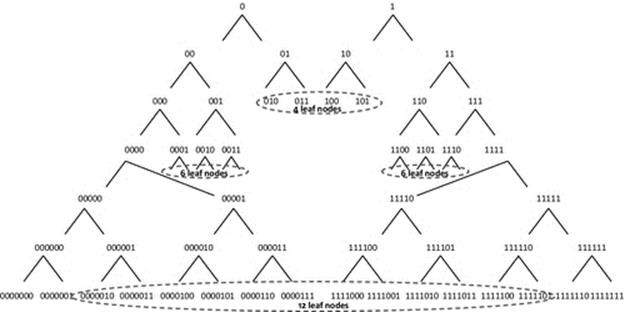
FIGURE 4.16 Binary tree to generate a 28-code set, which exhibits the prefix property.

The binary tree shown in Figure 4.16 has been arranged to generate 28 codes in which none of the codes are the prefix of any other codes in the set. This is achieved by only using leaf nodes as code values and allowing specific branches to continue down the tree until sufficient codes have been generated. This tree is extensible because four nodes have been left unused at the lowest level.

The next step is to place the letters of the alphabet and the space and full stop into a table in occurrence-frequency order and to assign the codes to the letters such that the shortest codes are allocated to the most frequently occurring symbols, as shown in Figure 4.17.

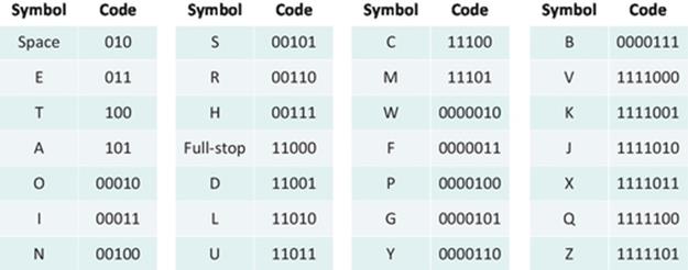
FIGURE 4.17 The codes assigned to symbols in occurrence-frequency order.

Notice that the code assignment in Figure 4.17 gives 3-bit codes to the most frequent symbols and 7-bit codes to the least frequent symbols. If a fixed length code were used, it would need to be 5 bit in order to generate 28 codes (it would actually generate 32 codes). Based on the code assignment shown in Figure 4.17, you should be able to decode the following message without ambiguity:

10000111011010000010000110011000001100011111101101000001000011000010000010001100110

1000000110010111011011111001011001010100001110001001110100101000011011000

4.6.2.3 Lossy Data Compression

JPEG (a standard created by the JPEG, from which it takes its name) provides a well-known example of lossy compression, specifically for digital images. JPEG supports adjustment of the compression ratio, which translates into a trade-off between reducing the size of the image file and maintaining the quality of the image. A compression factor of about ten can be achieved without significant reduction in image quality. Once compressed, some of the original data are permanently lost. As with all lossy compression, it is not possible, starting with the compressed image, to recreate the original full quality image.

4.6.3 Message Format

It is very important that the message is encoded by the sender in such a way that it can be decoded unambiguously by the receiver. For each field of data within the message, the receiver must know or be able to calculate the length and must know the data type.

Protocol data units (PDU) have been introduced in Chapter 3. To recap, a PDU is a message format definition that describes the content of a message in terms of a series of fields each with a name, an offset from the start of the message, and a length. This is important to facilitate the sender and receiver of a message synchronizing on the meaning and value of each field in a message. Protocol-level PDUs have specific names depending on the level of the protocol in the stack. Data link-layer PDUs are called frames, while network-layer PDUs are called packets, for example.

4.6.3.1 Fixed Versus Variable-Length Fields

The fields within a network message can have fixed or variable length. Fixed length is preferable generally because the boundaries between fields are determined at design time, simplifying aspects of the program logic that deal with messages, especially at the receiving side. Fixed-length fields also reduce the range of errors that can occur when populating fields with data and thus simplify testing. One further benefit of having the length of each field fixed is that the message itself has a fixed length, and thus, buffer memory allocation is simplified. In contrast, variable-length fields introduce the challenge (in the message receiver) of determining where one field ends and the next begins. If one or more fields have variable length, then the message itself has variable length making buffer memory allocation complex, especially at the receiver side as the buffer must be large enough to hold any message that arrives.

Variable-length fields are useful where there can be large variations in the actual length of message contents. However, because the data have a variable length, there needs to be an unambiguous means of determining the length of the field, at the receiving side. This is necessary both in interpreting the data in the field and in order to know where the next field begins. This can be achieved by either adding an additional field-length field or using an end-of-field termination character. Of these, the separate length field can be easier to implement but may require more bytes in the message. The end-of-field terminator must be a character or sequence of characters that cannot occur in the data part. The numerical value 0 (the ASCII NULL character) is often used (not to be confused with the character “0,” which has the ASCII code value 48). If data are ASCII-encoded, then the NULL character should not occur in normal text. In the specific case where an ASCII-encoded string is terminated with a numerical zero, the string is termed an ASCIIZ string.

The termination character approach requires additional processing to check through the field data until the end character or sequence is found. For variable-length fields where the field-data length has low variability, the additional design complexity combined with the processing overheads may outweigh the benefits.

Figure 4.18 shows three possible ways of representing the same three data fields. Each has some relative advantages and disadvantages. For example, the fixed-length field has the advantage of a simple fixed structure requiring no additional information or associated processing to describe the data. However, the field must be large enough to contain all possible values of the data, which can be very inefficient in highly variable data. Providing a separate length indicator solves the problem of having variable-length fields, but if the number is an integer, it adds two bytes (for an INT_16) and four bytes (for an INT_32) of overhead for each field and requires additional processing at both sender and receiver. The ASCIIZ representation is a well-known format that uses a termination character. It is an efficient way of representing variable-length data within a process but is far less convenient when used in a message because in addition to the individual fields being variable, the message length itself is variable, and the only way to determine the length is to read each field until the terminator is reached, to count the bytes, and to repeat until all the fields have been accounted.

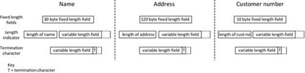
FIGURE 4.18 Comparison of different data representations: fixed-length fields, variable-length data with separate length indicator field, and variable-length data with termination character.

In summary, there is no single approach that will be ideal for all circumstances, but in a network-message context, fixed-length fields and thus fixed length messages are far easier to serialize and deserialize (see next section). As such, in any application where message field sizes tend to be generally short, I prefer to use fixed-length fields exclusively, thus trading some efficiency to achieve greater simplicity both in terms of code development and more significantly in terms of testing effort (because the size of all messages sent is preknown and thus the buffers can be allocated such that a message is guaranteed to fit within).

Fixed-length fields can be achieved using a single char array or byte array for the whole message and indexing into this as required, with specific index positions having specific meanings. A more flexible way to implement fixed-length fields is to define a structure to contain the message, which itself has a set of fixed-length data items. This predefined message format must be identified at both sender and receiver.

From a practical perspective, when developing in C or C++, it is ideal to place the message structure definition in a header file shared across both client and server projects; an example of this is provided in Figure 4.37 in a later section.

4.6.3.2 Application-Level PDUs

An application that sits above the network protocols, that is, uses the protocols in the stack to communicate application-specific messages across the network, will need to have one or more defined message formats. These message formats can be called application-level PDUs (this signifies that they are PDUs specific to the particular application and not defined universally in standards documents as are the protocol PDUs). Consider the case study application, the networked game of Tic-Tac-Toe; there will be a number of different messages, each sent either by a client to the server or by the server to one of the clients. Whichever part of the application receives the message must be able to interpret the message and extract the various fields of data back into the exact same form as they were held in at the sender prior to transmission.

4.6.4 Serialization

In the context of communication in distributed systems, serialization is the process of converting a structure or object into a linear byte format suitable for storing in a buffer and subsequently transmitting across a network. On receipt, the receiver will store the serialized data temporarily in a buffer and then deserialize it back into its native format. Serialization is also known as flattening, marshaling, and pickling.

In keeping with the game case study theme, consider the format of a message a game server could send to a game client to inform it of the current player scores; this is illustrated in Figure 4.19.

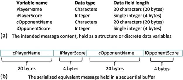
FIGURE 4.19 The concept of serialization, mapping data variables onto a sequential memory buffer.

Figure 4.19 shows a group of data variables relating to current game state, comprising the name and score of each of the players, to be transmitted by the game server as a single message. We can represent this data in the form of a structure, which can simplify the program logic and thus the coding. The C++-equivalent structure is shown in Figure 4.20.

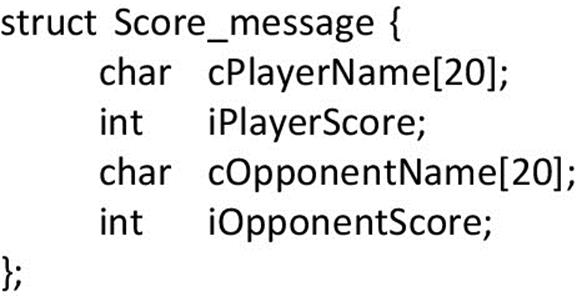
FIGURE 4.20 C++ structure holding game state information.

The C++ structure shown in Figure 4.20 contains only fixed-length fields, and thus, the structure itself has a fixed size. It will also be held in contiguous memory. These characteristics greatly simplify the serialization process. In C++, it is possible to use the structure memory directly as the buffer itself; a pointer to the start of the structure can be cast as a character array, and thus, the buffer is simply an overlay over the same memory that the structure occupies, without actually moving any data or changing any data types. The pointer and the size of the data structure (which is also the length of the buffer) are passed to the send primitive, and the message contents are transmitted as a stream of bytes, without the sending mechanism having to know the format or meaning of the individual bytes (see Figure 4.21).

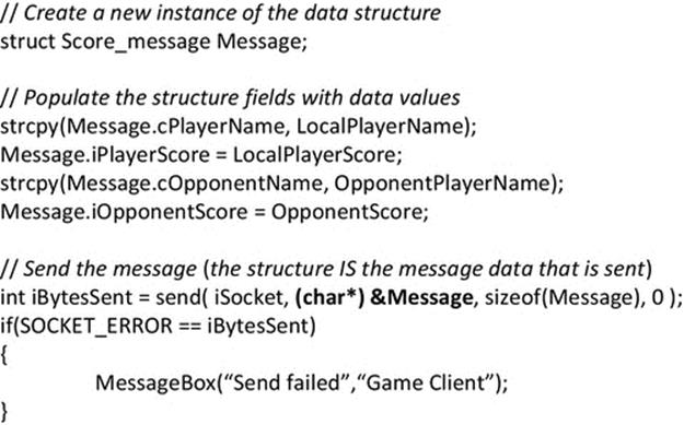
FIGURE 4.21 Serialization of a structure in C++ using a pointer and type cast (shown bold).

In some languages, serialization is not so straightforward, requiring the use of special keywords and/or methods that invoke mechanisms to perform the serialization, for example, in C# where the memory allocation is usually automatically managed and not under direct control of the programmer. In this regard, C# requires that the structure fields are allocated sequentially in memory (hence the use of “StructLayout(LayoutKind.Sequential)” in the example in Figure 4.22). The Marshal class provides methods for allocating and copying unmanaged memory blocks and converting between managed and unmanaged memory types. Python has “marshal,” which is a bare-bones serialization module, and “pickle,” which is a smarter alternative. Java requires that any class that is to be serialized “implements” java.io.Serializable. The ObjectOutputStream class is used to perform the actual serialization of the object.

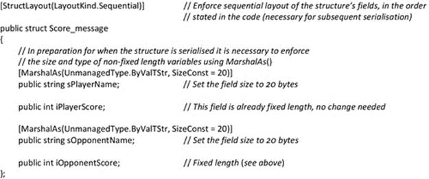
FIGURE 4.22 C# serializable structure holding game state information (compare with the C++ version in Figure 4.20).

C# automatically manages memory and uses dynamic memory allocation when creating certain data objects, including strings. This means that a programmer is not by default in complete control of the size of such objects. Also, because of the automatic memory management and the fact that strings may be extended dynamically, the various fields of a structure are not held in a contiguous block of memory. Thus, special mechanisms are needed to perform serialization. Firstly, a special mechanism (MarshalAs) is used to fix the size of strings within the structure; see Figure 4.22. Secondly, a serialization method is needed (Figure 4.23), which collects the various data fields into a continuous buffer format (a byte array) necessary for sending as a network message.

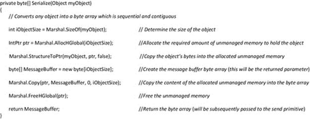
FIGURE 4.23 A C# method to serialize an object into a byte array.

Serialization is performed in the sending process, prior to the message being sent across the network. Upon receipt, the message will be placed into a message buffer, which is a flat byte array, prior to deserialization to recreate the original data structure so that the various fields of the message can be accessed. In C++, a similar technique of pointer casting (as was used for serialization) can be used to achieve this without actually moving the memory contents. For C#, deserialization is more complex due to the use of managed memory (as with serialization discussed above). An example C# deserialize method is provided in Figure 4.24.

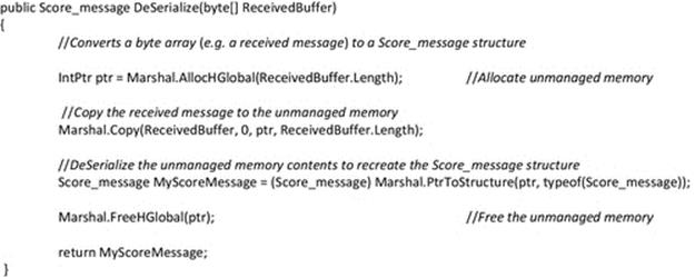
FIGURE 4.24 A C# method to deserialize (recreate) an object from a byte array.

In summary of this section, Figures 4.21 and 4.23 provide two quite different ways of performing serialization in order to show the variety of techniques used. The C++ technique shown is very simple fundamentally because the original data structure contains only fixed-length fields and thus it itself is a held in a fixed-length block of memory. In this case, the serialization is simply performed by treating the structure as a buffer, identified by its starting address and length. In contrast, in C#, special methods are required to perform serialization and deserialization principally because of the automatic management of memory allocation.

4.6.5 The Network as a Series of Links

First, we very briefly define the terms used to describe the various components of a network. A physical connection between two points in a system is called a link. A collection of such links is called a network. A particular path from one point in the network to another, possibly traversing several links, is called a route. The devices that are placed within the network, at the interconnection points, and responsible for finding routes are called routers.

Of particular interest to this discussion are the lower layers, especially the data link layer and the network layer. As their names suggest, these deal with passing data across links and networks, respectively. The data link layer operates on a single-link basis, transmitting data in a format called a frame to the point at the other end of the link. The data link-layer behavior and the frame format used are technology-specific, so they, for example, are different in Fast Ethernet and the IEEE 802.11 wireless LAN technologies. The network layer on the other hand is concerned with finding a route through the network comprising a series of links. This layer works independently of the actual link technologies; it is concerned with the link options that are available to it to enable data to be transmitted (in a format called a packet) from one part of the network to another.

The structure of networks is reflected in the ISO OSI seven-layer network model, which has been discussed in Chapter 3. Figure 4.25 relates the network devices discussed later in this section to the lower layers of this model and shows the PDUs, addressing schemes used at the various layers.

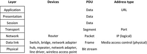
FIGURE 4.25 Network devices, PDUs, and address types related to the layers of the OSI network model.

The path between source node and destination node may comprise many devices including hubs, switches, and routers, but hubs and switches do not make routing decisions, so from a routing point of view, such devices are transparent. Another way to think of this is that routing decisions are made based on the addresses carried in IP packet headers (IP being a network-Layer protocol), and thus, routing is associated with the network layer. Hubs essentially boost signals but do not understand any type of address; hence, they operate at the physical layer only. Switches use media access control (MAC) addresses to select paths at the data link level and so are described as layer 2 devices.

The PDUs at the network layer are called packets, while at the data link layer, they are called frames. These have the same basic structure, comprising a header that contains information required by the network to transmit the PDU through the network and for the recipient node to understand the meaning and content of the PDU and a payload. The payload of the frame will be a packet (as illustrated in Figure 4.26). This is the concept of encapsulation, which has been discussed in more detail in Chapter 3.

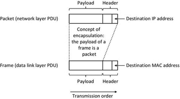
FIGURE 4.26 Encapsulation of a packet into a frame.

To transmit a packet across a network path comprising several links, a series of frames are used, one per link. The frame is used to carry the packet across a single link. On reception of a frame at a router, the packet is extracted from the frame, and the frame is discarded (as it was addressed to the specific router and thus has served its purpose). The router creates a new frame, addressed to the next router in the chosen route, and the original packet is re-encapsulated into the new frame, which is then transmitted onto the outgoing link.

Switches do not understand IP addresses, and thus, a switch that lies in the path between a pair of routers will forward frames from one router to another at the link level based on the MAC-level addresses of the routers and does not influence the higher-level routing activity. This is illustrated in Figure 4.27.

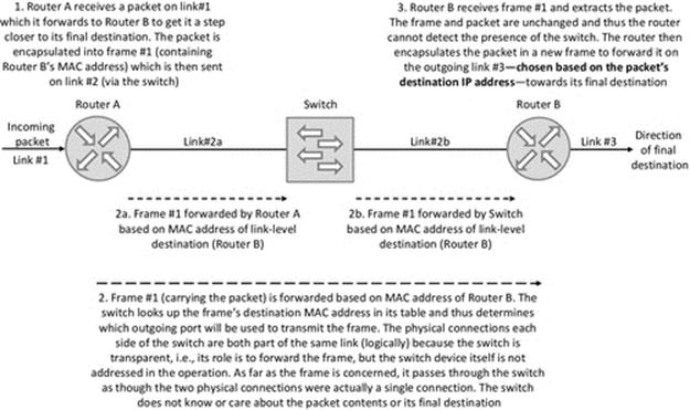
FIGURE 4.27 Combined use of MAC addresses within frames and IP addresses within packets to transmit a packet over a series of links.

Figure 4.27 illustrates how the entire system of links between the two routers appears as a single link to the network layer. This is because a packet is transmitted across this system of links unchanged. The routers cannot tell if there are zero, one, or more switches in the path; thus, the switches are said to be transparent to packets and the network layer.

4.6.6 Routers and Routing

Routers are specialized computers that direct network traffic and thus have a large influence on the effectiveness of message transmission. Therefore, it is important for developers of distributed applications to understand the basic concept of their operation.

Networks are highly dynamic environments. Dynamic behavior arises primarily from changes in the types and volumes of traffic flowing, which is driven by the different types of applications being used, by different numbers of uses at different times. In addition, links and routers and other devices can fail and be repaired unpredictably, changing the availability of routes and the total capacity of parts of the network from time to time. New devices and links are added, computers and services are upgraded, and so forth. The router has to choose the “best” route (see below) for a given packet, very quickly, despite the high level of dynamism.

The router keeps track of its knowledge of available routes and current network conditions in a routing table, which is updated frequently to reflect the dynamic characteristics of the network. When a packet arrives at a router, the router will inspect the destination IP address in the packet header. Based on the destination address and the current state of the routing table, the router will select an output link on which to pass the packet, with the goal of moving the packet one step (one “hop”) closer to its destination.

This is illustrated in Figure 4.28. Part (a) of the figure shows a core network of seven routers (i.e., it does not show the various devices such as switches and computers that are connected to routers at the periphery of the network). Part (b) of the figure shows the routing table for Router B. The routing table forms a link between three pieces of information that the router uses to route packets: the destination network address of the particular packet (which it reads from the packet's header and uses as an index into the table); the outgoing link that represents the best known route (in this example, it is based on the number of hops to the destination); and the actual distance of the current best known route (this is necessary so that if a new possible route for a particular destination is discovered, the router can determine if it is better than the current one held).

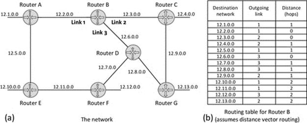
FIGURE 4.28 A core network of seven routers and the routing table for Router B.

The router's use of the routing table is illustrated with a couple of examples: (1) A packet arrives from Router A, with a destination network address of 12.13.0.0. The router looks up the destination address 12.13.0.0 and finds that the current best known route is via link 2. This means that the packet will be passed to Router C. 2. A packet arrives from Router D, with a destination network address of 12.1.0.0. The router looks up the destination address and finds that the current best known route is via link 1, so the packet is passed to Router A.

In distance vector routing (which is the basis of the example shown in Figure 4.28), each router only has partial knowledge of the entire network topology and does not have to know the full configuration of all routers and links. In this case, Router B does not need to know the actual connectivity beyond its immediate neighbors, but through the exchange of routing protocol messages with its neighbors, it will learn the best routes (in terms of the outgoing links to use) to the destinations.

The actual way in which the router chooses the output link is determined by the actual routing protocol in use and the actual metrics used by that protocol, which define what is meant by “best” route (e.g., the least number of hops, least loaded, and most reliable). In some cases, there will only be one output link that can move the packet on its way in the right direction, so regardless of the routing protocol, this link will be chosen. Things are more complex when there are many possible routes to choose from and where the network traffic conditions are highly dynamic, leading to fluctuations in link utilization and queue lengths in the routers themselves. Under such circumstances, it can be difficult to predict which link the router will select for any specific packet and two consecutive packets sent by the same source node and heading to the same destination node may actually be passed along different links by a given router; see Figure 4.29.

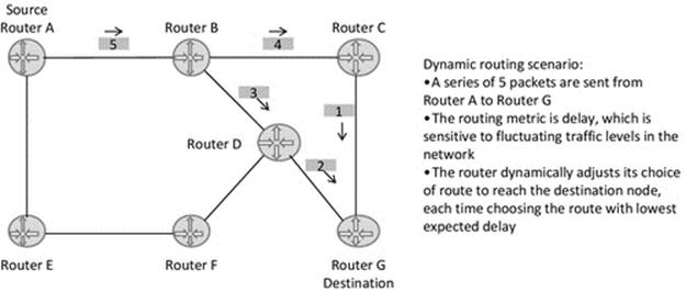
FIGURE 4.29 Dynamic route determination based on network conditions.

Figure 4.29 illustrates dynamic routing in which packets with the same source and destination addresses are passed along different routes. This can lead to different delays to the packets as they encounter different congestion on each route. It is also possible that the arrival order of the packets will be changed by each taking different routes. Referring to the example in the figure, the second packet sent (labeled 2) may arrive at the destination before the first packet that was sent (labeled 1).

As discussed earlier, layer 1 and 2 devices are transparent to routing, that is, they do not affect the route taken, and thus can be ignored for the purpose of packet routing. From the perspective of a packet moving from source to destination, its path can be described in terms of the routers it passes through, as it is only at these points that its path can change. Each time a packet is passed from one router to another, it is deemed to have traveled one “hop.” Essentially, each router represents a queue. This is because the outgoing link can only transmit packets at the fixed rate, which is determined by the link technology (so, e.g., if the link technology is Fast Ethernet, the router will transmit onto the link at a rate of 100 Mb/S, and thus, a packet of 1000 bits will take 1000 bit times to transmit. In this case, a bit time is 10^{− 8} s. The transmission time is thus 10^{− 8} × 10³ = 10^{− 5} s = 10 μS). If packets destined for a particular outgoing link arrive at the router faster than the rate at which the router can transmit them, then a queue forms. It is important to realize that the time taken to process the queue depends on both the bit rate of the outgoing link and also the length (number of bits) of each packet. If the buffer is empty when the packet arrives, it will start to be transmitted straight away. However, if there are other packets in buffer already, the new packet has to wait.

The end-to-end route is effectively a series of queues the packet must move through, and the total queuing delay is the sum of the delays in each of these queues; see Figure 4.30.

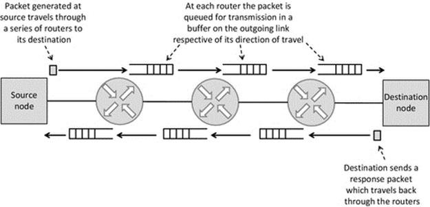
FIGURE 4.30 Resource view of a network route; a series of queues.

As shown in Figure 4.30, a packet moves through each queue in sequence until it reaches the destination. The length of the queues is resultant of the amount of traffic flowing on the various links, and when there is more traffic, the mean queue lengths increase; this is commonly described as congestion.

Figure 4.31 illustrates the way in which congestion builds up as the result of many different traffic flows, which combine (share links) at different points in the network, and thus, the congestion is both dynamic and nonsymmetric. In the example shown, traffic flows 1 and 3 share part of the same route as the application flow (shown as the darker, fine-dotted line) between the source and destination nodes highlighted and thus impact on the lengths of the queues on router output links that the application flow uses.

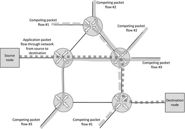
FIGURE 4.31 The combined effect of many traffic flows gives rise to complex traffic patterns.

It is very important that as designers of protocols and applications, we understand the nature of this congestion and the way it builds up and the way it affects the delay and packet loss levels encountered by messages sent within our applications. The simplest observation is that a buildup of queues in the path of a packet means that the packet will take longer to travel through the system. The router is itself a specialized computer, and it has to process each packet in turn and transmit it onto the appropriate outgoing line. The router operates at a finite speed, and the outgoing line has a finite bit rate. For a specific packet, the transmission time onto the outgoing line is directly proportional to the length of the packet. However, the time spent in the queue is dependent on the number of packets already in the queue, which must be processed ahead of our specific one.

The router also has a finite amount of memory, in which it can store packets. This is organized as buffer space, and there may be a separate buffer designated for each output link. The finite aspect of the buffer leads to another important observation; the buffer will eventually fill up if packets arrive quickly to the router, faster than they can leave. This is analogous to vehicles arriving at a road junction at a busy time of the day. If the vehicles join the end of the queue faster than they leave the front of the queue, then the queue will get longer and longer. This fact is well known to everyone who drives in a city during the rush hour. Once the rush hour is over, the queues reduce quickly, because there are far less vehicles joining the queue per unit time, but the number of vehicles that are able to leave the queue per unit time (i.e., by entering the junction) does not change.

Each packet that arrives at a router must be held in memory while it is processed. If the buffer is full (the queue is full), the router has to ignore the packet; that is, it cannot store the packet because there is nowhere to put it, so the packet ceases to exist. This is termed “dropping” the packet and is a main cause of packet loss in networks. The term packet loss can lead to some misunderstanding; people sometimes talk about packets being (or getting) “lost,” which might imply that the router was careless and mislaid them somehow or that it directed them to the wrong destination, implying that the cause of the loss was linked to the packet address and the processing thereof. It is very important to realize that in fact, most loss is linked to congestion and finite buffers in routers; this motivates us to find appropriate ways to minimize this loss or design protocols or applications to be less sensitive to it and/or to be more efficient in transmission so that less traffic is generated.

Note that it is the finite characteristic of memory buffers in routers that is the fundamental problem we have to address. Put another way, no matter how large the buffer is, it will always fill up given enough congestion. I have heard many arguments for making buffers larger, in the hope that this will solve the problem of packet loss. However, larger buffers allow the queue to build up longer before packets are dropped, which translates into more delay for the packets that are in the queue and longer time required for the queues to clear after a period of congestion. This last point is significant because much network traffic has a “bursty” nature³, and enabling longer queues to build up can cause the effect of a sudden burst of traffic to impact on the network performance for longer after the event. Optimization of router queue lengths is itself a complex subject due to the number of dynamic factors involved, but it is important to realize that facilitating longer queues does not necessarily translate into better performance; the salient point is that it all depends on which performance metric is used; packet loss is traded against packet delay.

4.6.7 Overheads of Communication

The transport layer provides a good example of the way in which trade-offs can arise in the design of protocols. Two very well-known protocols are provided in the transport layer, namely, TCP and UDP as discussed in Chapter 3.

The choice of transport protocol is of interest from a resource viewpoint because it can have a significant impact on communication overheads. TCP is described as a reliable protocol. This is warranted because TCP has a number of mechanisms, which ensure that segment loss is detected and the affected segments are retransmitted. In addition, duplicate segments are filtered out at the receiver node, using the in-built sequence numbers. TCP also implements flow control and congestion control mechanisms, which further enhance robustness. Each of these features adds overhead, in terms of additional fields in the TCP header, transmission of acknowledgments, and additional processing at both sender and receiver nodes. UDP in contrast is a basic transport protocol without any mechanisms to enhance reliability and is thus described appropriately as unreliable.

In addition to the overheads, TCP also introduces additional latency because of the need to establish a connection prior to transmitting data. UDP can send a datagram immediately without the need for a connection to be established or any other handshaking.

There are many categories of distributed application for which reliable transport is mandatory, that is, where no message loss can be afforded. For these applications, TCP must be used. However, there are some applications where some message loss is acceptable, especially if this is accompanied by lower communication overheads and lower latency. The benefits of TCP's reliability are reduced when the communicating nodes are within the same local area network as there is less likelihood of packet loss, especially where there is no router between the nodes, so no possibility of being dropped from a queue. UDP has the advantage of being able to perform broadcasts, although these are blocked at the edge of the local broadcast domain by routers. UDP is thus popular for local communication scenarios such as service discovery.

4.6.8 Recovery Mechanisms and Their Interplay with Network Congestion

Reliable protocols, such as TCP, have in-built recovery mechanisms, whereas unreliable protocols such as UDP do not. This is a main criterion when selecting the most appropriate protocol for a particular application.

There is a complex interaction between recovery mechanisms and congestion. Firstly, congestion leads to queues building up, and eventually when buffers are full, packets are dropped, as discussed earlier. A recovery mechanism will detect the loss of a packet, by the fact that the packet does not arrive at the destination and subsequently that the sender does not receive an acknowledgment. The recovery mechanism then retransmits the packet, which adds to the traffic in the network. In some situations, this could lead to perpetuation of the congestion conditions.

Figure 4.32 illustrates the communication mechanism view of end-to-end transmission of TCP segments (carried in IP packets) and the resulting return of acknowledgments. Solid arrows show the network-layer path determined by the IP forwarding actions of the routers. Dotted arrows show the logical view, at the transport layer, between socket end points in processes at the source and destination computers.

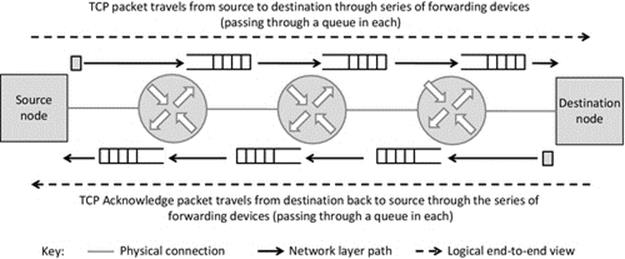
FIGURE 4.32 End-to-end acknowledgment as implemented in TCP (communication mechanism view); the situation without congestion.

Figure 4.33 illustrates the timing behavior view of end-to-end TCP transmission and the resulting return of acknowledgments. The timer is used as a means of detecting a lost packet; it is configured to allow enough time for a packet to reach the destination and for an acknowledgment to propagate back (this is the Round Trip Time (RTT)), plus a safety margin. The timer is canceled on receipt of the expected acknowledgment. If the transmission has not been acknowledged at the point when the timer expires, then the packet is considered lost and it is retransmitted. Under normal circumstances (when packets are not lost), the timer gets canceled and no retransmission occurs. However, networks are highly dynamic generally, and thus, the end-to-end delay can vary significantly, even over short timeframes. This makes setting any fixed timeout period problematic and so TCP automatically adjusts its timeout based on recent RTT values in an attempt to compensate for the variations in delay.

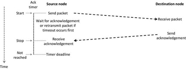
FIGURE 4.33 End-to-end acknowledgment as implemented in TCP (timing behavior view); the situation without congestion.

Figure 4.34 illustrates the effect of congestion on packet transit. Queues operate independently at each router, thus the congestion can occur in one direction or both directions. This leads to two different failure modes: An outward packet could be dropped, in which case the destination node will not generate an acknowledgment (scenario A in Figures 4.34 and 4.35), or the outward packet may be delivered and the acknowledgment that is sent back could be dropped because of a full buffer (scenario B in Figures 4.34 and4.35). In each case, the source node will retransmit the packet when its timer expires, and in the scenario A, the new packet is the only one to arrive at the destination. However, in scenario B in which it was only the acknowledgment that was lost, the new packet arrives at the destination as a duplicate. TCP resolves this further issue by placing sequence numbers in each packet. Such aspects of protocol behavior are discussed in depth in Chapter 3; here, the focus is on resource issues.

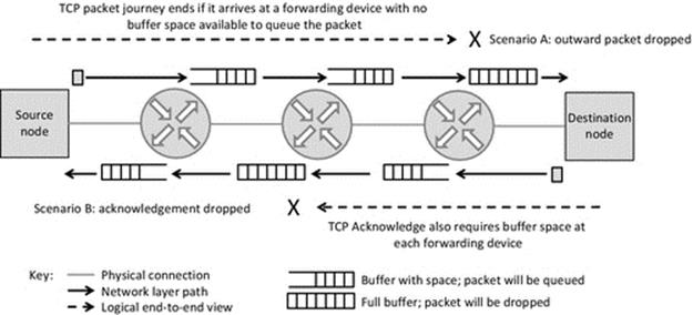
FIGURE 4.34 End-to-end acknowledgment as implemented in TCP (communication mechanism view); the situation with congestion.

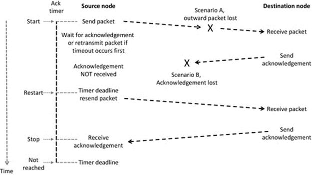
FIGURE 4.35 End-to-end acknowledgment as implemented in TCP (timing behavior view); the situation with congestion.

The timing diagram in Figure 4.35 assumes that congestion is short-lived and that the retransmitted packet is successfully delivered and acknowledged. However, in heavily congested networks, a whole series of retransmissions may be lost due to full buffers, and in such case, the retransmission mechanism is adding to the problem; it is adding packets to the queues upstream of the congestion and consuming processing resources of the forwarding devices, as well as wasting network bandwidth. The further along the round-trip the congestion is from the source node; the more resources are wasted. To prevent an infinite perpetuation of traffic in such circumstances, protocols such as TCP have a configurable maximum retransmission count, and when this is reached, the protocol signals the layer above reporting that the transmission has failed.

Recovery of lost packets has resource implications and, as with almost every aspect of protocol design, involves trade-offs. The application designer needs to bear in mind the functional and nonfunctional requirements of applications when choosing the appropriate approach and be aware of the network overhead incurred by retransmission. The most general trade-off is between communication robustness and efficient use of bandwidth and queue buffers within the transmission path. The recovery of lost messages also increases end-to-end delay at the application level. This represents a trade-off between responsiveness and data completeness. For data applications such as file transfer or online transactions, the data completeness is paramount, so recovery using a reliable transport protocol is vital. In contrast, recovery is not usually beneficial in real-time applications such as live audio or video streaming. The retransmitted data may arrive too late to be useful and potentially increase jitter and delay.

There are some applications that send low-value periodic messages, the loss of some of which can be tolerated without recovery. For example, many services send heartbeat messages, which serve to inform the rest of the system that the particular sending component is still healthy. If there is a period where none of these messages are received by other components, one of the others will instigate an application-level recovery, for example, by starting another instance of the missing service. Such mechanisms are typically designed such that a heartbeat is sent every few seconds and that perhaps five such messages in sequence must be omitted before action is taken. Thus, each message is individually dispensable without recovery. Another example would be a periodic clock synchronization message, which could, for example, be transmitted once per minute. Even with the lowest-accuracy local clock technology currently available, the clock drift over several minutes would be very small, and thus, one of more of these messages could be lost without having any discernible quality impact on the service provided.

In situations where some message loss is acceptable or where the latency associated with recovery is undesirable, it may be appropriate to choose a simpler transport protocol such as UDP rather than a more complex protocol such as TCP, which has a significant management overhead.

4.7 Virtual Resources

This section describes a number of resources that are necessary to facilitate communication and thus on which the operation of distributed systems and applications is dependent. These resources can be considered to be virtual in the sense that they are not tangible; for example, a port number is a numerical value and a specific port can only be bound by a single process at a particular computer.

4.7.1 Sockets

Sockets are the end point of communication. A process needs at least one socket to communicate; however, it can use as many as necessary to manage the communication effectively. The program logic is generally clearer if there is one socket dedicated for communication with each of its communication partners. An important example of this is when a server process accepts many connections from clients, using TCP. “Listen” need to only occur once (at the server), and thereafter, clients can attempt to “connect” to the server. The “accept” primitive can be placed in a loop on the server side such that each time a client connection request is accepted, a new socket is created for the server's communication with that particular client. This can greatly simplify the communication logic, as the socket itself is a means of identifying which client is being communicated with; a socket has a numerical value and is created and managed by the operating system.

4.7.2 Ports

Ports are an extension of addressing in the transport layer of the TCP/IP protocol stack. Specifically, a port number identifies a particular process at a particular computer (identified by its IP address) or can be used to address a set of processes that are using the same port but with different IP addresses (i.e., on different computers). This latter usage is ideal with broadcast communication, which can be facilitated, for example, with UDP.

The port number identifies which process the message carried by either a TCP or UDP segment should be delivered to. Recall that the IP address carried in the network-layer header identifies the computer that the message should be delivered to. The combined IP and port number addresses are written in the form IP address:port, for example, 192.56.64.3:80.

Processes are already uniquely identified at each computer by their process ID (PID). However, this value can be different each time the process runs, because they are allocated dynamically by the operating system, usually in round-robin sequence. This means that they are not predictable and cannot be used by another process as a means of addressing the target process. In contrast, port numbers are preknown values independent of the PID. The operating system has to maintain a mapping between the two types of identifier, in a dynamic table, so it knows which process a particular message (addressed by port number) should be passed to.

A port number is a 16-bit value. The port number may be chosen by the developer, taking care to avoid the reserved ranges of values for well-known services, unless the application is such a service. So, for example, if a Telnet service is being developed, the port 23 should be used. Notice that this only applies to the service (server) side of the communication. This is so that the client will be able to find the service.

A process requests to use a particular port number via the “bind” system call. If the operating system permits the process to use the requested port, it adds an entry into a table, which is subsequently used to match an incoming message to the appropriate process. There are two main reasons why the use of a requested port may be refused. Firstly, a process may not be authorized to use the port if it is in the reserved (well-known) range; secondly, the port may already be in use by another process located at the same computer.

4.7.3 Network Addresses

This section briefly discusses network addresses from the resource viewpoint.

IP addresses are described as logical addresses because they are chosen so as to collect computers into logical groupings based on connectivity and the structure of networks. The IP address has a hierarchical format comprising network part and host part. This is vital so that routing algorithms can make packet-forwarding decisions without having to know the actual physical location of individual computers or the full topology of networks. IPv4 addresses are 4 bytes long each, which means that every IPv4 packet contains 8 bytes of IP address (destination address and source address). This is a relatively small overhead when compared with IPv6 addresses, which are 16 bytes each, and thus, addresses take up 32 bytes of every IPv6 packet. A computer can have multiple IP addresses. Routers in particular have a logical presence in each network they are directly connected to, so they need to have an IP address for each of these networks.

Media control access (MAC) addresses are described as being physical addresses because they provide a globally unique identification of a specific network adapter and thus of the host computer. The address remains the same regardless of where the computer is located. A computer can have multiple network adapters; for example, it may have an Ethernet adapter and a wireless network adapter, in which case it would have two MAC addresses. MAC addresses are ideal for local link communication between devices. They are unsuitable as a basis for routing because routers would need massive memories to hold the routing table; essentially, the router would have to know explicitly how to reach each specific computer. In addition to the memory size problem, there would be the associated time required to search through the memory and also the serious overhead of keeping the table up-to-date, which would be effectively impossible now that mobile computing is so popular and devices change physical locations regularly. MAC addresses are typically 6 bytes (48 bits) although this is dependent on the actual link-layer technology. MAC addresses thus account for 12 bytes of every frame transmitted (destination MAC address and source MAC address).

4.7.4 Resource Names

Resources such as files and objects that are located within a distributed system need to have names, which are independent of their location. This means that the resource can be accessed by only knowing its system-wide unique name and without the need to know its physical location.

The uniform resource identifier (URI) provides a globally unique identification of a resource, and the uniform resource locator (URL) describes how to find (locate) the resource. The difference between these is often overlooked, and the terms are often used interchangeably, but strictly URLs are a subset of URIs.

URLs often contain a host name, which is mapped into the name space of the domain name system (DNS), which means that they can be looked up and translated into an IP address by the underlying access mechanisms wherever needed in the system. DNS is discussed in Chapter 6.

There are several forms of URL used with different classes of resource such as email inboxes (so an email can be sent to your inbox without knowledge of the IP address of the host computer) and similarly for files, hosts, and web pages. A URL has the generic form:

protocol://host-name/path/resource-name

where protocol identifies the type of service used to access the resource, such as ftp or http; the host-name field can contain an IP address and an optional port number or a DNS name space entry—in either case, it uniquely identifies the host that holds the resource; path is the location of the resource on the host computer; and the resource name is the actual name of the resource, such as a filename.

Some examples of URLs are provided in Figure 4.36.

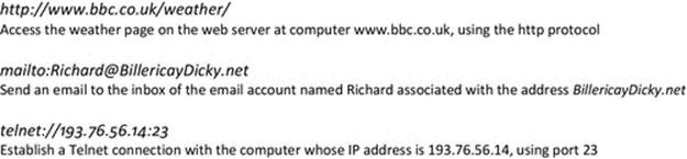
FIGURE 4.36 A selection of URL format examples.

4.8 Distributed Application Design Influences on Network Efficiency

Designers of distributed applications need to be well informed with respect to the way in which design choices affect the use of resources and the efficiency with which the resources are used. They need to be aware of the ways in which the performance and behavior of applications are impacted by the design of the underlying networks and the dynamic traffic characteristics of those networks and also to be aware of any specific sensitivities of their applications to issues such as congestion and resource shortages.

Designers need to keep in mind the finite nature of critical resources in systems and that typically there is competition for key resources from other applications present. The design of distributed applications should take into consideration the fact that applications share these resources and that the behavior of their application adds to the level of congestion in networks (and thus impacts indirectly on the performance of other applications in the system).

A main challenge is that at design time, it is not possible to know the various configurations of run-time systems in terms of architecture, resource availability, and the loading on those resources. The safest approach is to build distributed applications that are lean and efficient in terms of resource usage. This enhances their own performance and scalability as they are better able to operate when resource availability is restricted or fluctuates, as is common in networks when traffic levels change continuously, causing changes in delay and packet loss levels. Resource-hungry applications fare worse in busy systems and also impact more severely (through competition for resources) on other applications.

This chapter has identified a number of resource-related challenges and techniques for ensuring applications are efficient with respect to resource use. Communication design aspects should be first-class concerns when designing robust and efficient distributed systems. Aspects to consider include the choice of transport protocol (because of the trade-offs between reliability, overheads, and latency), cautious use of local broadcasts, data compression prior to transmission, careful design of message format and size, and the frequency and pattern of sending messages, taking into account the possibility of data aggregation where appropriate.

4.9 Transparency from the Resource Viewpoint

The forms of transparency that are particularly important from the resource viewpoint are briefly identified here and are examined in more depth in Chapter 6.

4.9.1 Access Transparency

Resources that are remote to a process must be accessible by the same mechanisms as local resources. If this form of transparency is not provided, application developers must build specific mechanisms, and this can restrict flexibility, portability, and robustness.

4.9.2 Location Transparency

Developers should not need to know the location of resources. Naming schemes such as URLs, in combination with name services such as DNS, enable the use of logical addresses and remove the need to know the physical location.

4.9.3 Replication Transparency

Resources are often replicated in distributed systems to improve access, availability, and robustness. Where this is done, the resources must be accessible without having to know the number of or location of the actual copies of the resource. For example, updating a single resource instance should cause mechanisms in the system to automatically update all other copies. Techniques to achieve replication transparency are presented in Chapter 6.

4.9.4 Concurrency Transparency

Where resources are shared by concurrently executing threads or processes, it is vital that the values of the resources remain consistent. Problems arising from unregulated interleaved access to resources can corrupt data and render a system useless, so must be prevented using mechanisms such as locks and transactions.

4.9.5 Scaling Transparency and Performance Transparency

The network is a fundamentally key resource for distributed systems. The network is a shared resource and the bandwidth is finite. Careful design of communication aspects of distributed applications is an important contribution both towards high scalability and also towards maintaining high performance as scale increases.

4.10 The Case Study from the Resource Perspective

The case study game is not particularly resource-intense. It does not require a lot of processing power and also does not send very much data across the network. Nevertheless, it must be designed to be efficient and therefore to be scalable, to have low impact on the availability of the resources in the system, and also to be minimally impacted by the demands on resources made by other processes.

It was decided to implement the game directly on top of the TCP protocol and not use UDP. The primary reason for this decision was the fact that every message sent is critical to the operation of the game, so if TCP were not used, then application-level message-arrival checking would have to be implemented in any case and this would incur significant additional design and testing cost. Additional reasons include that the game does not have any real-time performance requirements and so would not benefit from the end-to-end latency improvements that UDP may be able to achieve. The communication within the game occurs at a low rate (see discussion below) such that the additional overheads incurred by using TCP are negligible. Finally, the game has no requirement for broadcasting, further confirming the case for avoiding UDP.

A number of message types have been identified, used to indicate the meaning of messages passed at the various stages within the game. Message types include the client registering a player's chosen alias name with the server (REGISTER_ALIAS), the server sending and updating to clients a list of connected players (PLAYER_LIST), a client selecting an opponent to play against from the advertised list (CHOOSE_OPPONENT), the server signaling the state of a game to clients (START_OF_GAME), the server signaling game moves from one client to the server and then from the server to the opponent client (LOCAL_CELL_SELECTION, OPPONENT_CELL_SELECTION), the server informing clients of the outcome of a game (END_OF_GAME), and a message to enable clients to disconnect gracefully (CLIENT_DISCONNECT).

Enumerations are used in the definitions of message type and also message code type (which is used when signaling the end-of-game status). This is a much better alternative to defining constants as it collects the related definitions together and improves the readability and maintainability of code.

The message PDU is defined as a structure and contains the message type enumerator (which is essentially an integer value) that is set appropriately prior to sending the message. This greatly simplifies the message receiving logic, as a switch statement can be used to process the message type value and thus handle the message accordingly. The enumerations and message PDU structure are required when compiling both the client and server application codes. As the game was written in C++, it is ideal to place these commonly needed definitions into a header file, which is then included into both the client and server code projects. The contents of the header file are shown in Figure 4.37.

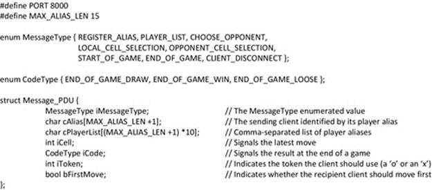
FIGURE 4.37 C++ header file, which defines the message types and PDU format for the game.

Figure 4.37 shows the single PDU format used for all messages in the game. It contains a number of fixed-length fields, and thus, the message itself always has a fixed length. This approach simplifies design and implementation and testing. It ensures that both sides of the communication (client and server) have predefined message structures and statically allocated message buffers, and there is no need for additional processing to calculate message sizes or field boundaries within messages. Testing is simplified because the fixed-length approach prevents certain failure modes, for example, the message size is too large for the receive buffer, or another common mistake is that a termination character was overwritten or omitted.

The single PDU contains all of the data fields each time it is sent, but each of the various message types only uses a subset of these as necessary. This can be justified in terms of the trade-off between a more complex multi-PDU design that reduces the individual message sizes and the simpler more robust design achieved here. The game logic is quite simple and the game play is not communication-intense, the rate of sending messages being determined mainly by the user's thinking time to make their move selection. Typically, one move might be completed every 5 s or so, causing one message to be sent to the server from the player's client and a corresponding update message being forwarded to the opponent's client, which also serves as a means of informing the opponent that it is their turn (and allowing the user interface to accept a move). This represents a form of message aggregation as two logical messages are combined into a single transmitted message. The application-level communication load is thus two messages per user action (the one sent to the server and one sent by the server to update the other client).

A single PDU format has a size of 196 bytes. If PDUs were repeatedly sent at a rapid rate, such as in a high-action game, then there would be a strong argument for separation into a number of message type-specific PDUs, which are smaller, especially removing the single largest field of cPlayerList (160 bytes) from the messages where it is not needed.

TCP/IP encapsulation adds overheads of the TCP segment header, which is typically 20 bytes, and the IP packet header, which is also typically 20 bytes, and if connected over an Ethernet network, the 18 byte Ethernet frame header must also be added. Thus, the actual size of each transmitted message taking into account encapsulation through the layers is 196 + 20 + 20 + 18 = 254 bytes, which is equivalent to 2032 bits, and the total for the two messages sent at each activity is thus 4064 bits.

However, with messages being transmitted only every 5 s or slower, the total bandwidth requirement of this game is a maximum of 813 bits per second which is very low. To place this in context with typical bandwidth availability, it represents approximately 8 millionths of the total bandwidth of a Fast Ethernet link. In this case, the simplifications of having a single PDU format were deemed to outweigh the benefits of optimizing the message size further.

As with all distributed applications, there is a need to ensure data consistency. The game has been designed such that the server maintains all game state information. Clients only have indirect access to the game state through defined interactions on the communication interface with the server, so they cannot directly update it. Thus, so long as the server code is designed carefully, there should be no consistency issues, especially as it is single-threaded. If the server were multithreaded, where each thread handled a single client (which is a common design in many server systems), then maintaining consistency across the threads would need consideration. Also, if the server were replicated and shared its state across multiple server instances, then consistency issues could arise.

Nonblocking sockets have been used in both client and server. When a game is in progress, the server will have at least two connected clients, each using a different socket on the server side. The use of nonblocking sockets removes any issues that could arise from specific sequences of messages, for example, if the server process was blocked on one socket and a message arrived on the other. In the client side, the use of a nonblocking socket ensures that the user interface remains responsive while waiting for messages to arrive. The application logic is sufficiently simple in this case that a single-threaded approach in combination with nonblocking sockets achieves the necessary responsiveness without the additional complexity of designing and testing a multithreaded solution.

Port numbers. It was decided to design the game in such a way that all three run-time components in a minimum single-game scenario (the server process and two client processes) could coexist on the same computer to simplify some aspects of testing and also for some demonstration purposes. Obviously, to play the game in the distributed form as intended, each user (and thus each client process) would be located on a different computer. Even in this case, it is still desirable that the server and one of the clients can be colocated. To support two or all three components being colocated on the same computer, it is necessary to ensure that they do not all attempt to bind to the same port number. By using TCP as the transport protocol, it is only necessary for the server to bind to a specific port known to the clients so that they can issue TCP connect requests. The client processes do not need to explicitly bind to any ports because they only receive messages within established TCP connections.

4.11 End-of-Chapter Exercises

4.11.1 Questions

1. PDUs and serialization

(1a) Create a suitable PDU format to hold the following data:

Customer name = Jacob Jones

Customer age = 35

Customer address = 47 Main Road, Small Town, New County, UK

(1b) Provide an illustration of the serialized form of your PDU; state any assumptions that you make.

(1c) Based on your PDU design and means of serialization, describe how the receiver will perform deserialization. Is there enough information for the received data to be extracted to reconstruct the original data format? If not, revisit part (1a) and modify your scheme.

2. PDUs and message types
Consider a PDU containing the following fields:

char Customer ID [8];

char Customer name [100];

char Customer address [200];

char Customer Phone number [15];

This single PDU format is used in two different message types:

• Retrieve full customer details

• Retrieve customer phone number

(2a) Identify the two issues arising from this single PDU design: one relating to efficiency and one relating to message identification.

(2b) Design new PDU formats to resolve the issues identified in part (2a).

(2c) Now that there are multiple PDUs, is it possible for the receiver of a message know in advance how much memory to reserve as a buffer?

3. Dynamic memory allocation
Consider the three dynamic memory allocation scenarios shown in Figure 4.38.

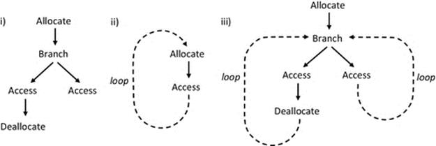
FIGURE 4.38 Dynamic memory allocation scenarios.

(3a) Assuming that there is no automatic garbage collection (as, e.g., in C and C++), evaluate the consequences of the three scenarios given.

(3b) If automatic garbage collection is present (as, e.g., with Java and C#), how does this affect the situation?

4.11.2 Exercises with the Workbenches

Exercise 1: Understanding the “lost update” problem (part 1: the fundamental problem)

The exercises below use the “Threads—Threads and Locks” application within the Operating Systems Workbench to investigate the lost update problem.

1. Inspect the initial value of the data field.

Q1. If one thousand increment updates are performed, what value should it end up at?

2. Click the “Start ADD Thread” button to run the ADD thread in isolation.

Q2. Was the result as expected?

3. Note the value of the data field now.

Q3. If one thousand decrement updates are performed, what value should it end up at?

4. Click the “Start SUBTRACT Thread” button to run the SUBTRACT thread in isolation.

Q4. Was the result as expected?

Q5. If the threads are run sequentially (as above), are there any issues concerning access to the shared variable that can lead to its corruption?

5. Click the “Reset data field” button to reset the value of the data variable to 1000.

Q6. Given a starting value of 1000, if one thousand increment updates are performed and one thousand decrements are performed, what should the final value be?

6. Click the “Start both threads” button to run the two threads concurrently.

7. When both threads have finished, check their transaction counts to ensure both executed 1000 transactions; hence, determine the correct value of the data variable.

Q7. Is the actual data variable value correct? If not, what could have caused the discrepancy?

Exercise 2: Understanding the “lost update” problem (part 2: exploring the nature of the problem)

The lost update part 1 activity exposed the lost update problem. We saw that a discrepancy occurred between the expected value and the actual final value of a shared variable. Some of the updates were lost. This is because one thread was allowed to access the variable, while the other had already started a transaction based on the value of the variable.

Q1. How does this problem relate to transactions in database applications?

Q2. How many of the ACID properties of transactions have been violated?

Q3. How could this problem affect applications such as

an online flight-booking system?

a warehouse stock-management system?

Q4. Think of at least one other real-world application that could be affected by the lost update problem?
Investigate the nature of the problem. Repeat the following steps three times:

A. Ensure that the value of the data variable is 1000 (click the “Reset data field” button if necessary).

B. Click the “Start both threads” button to run the two threads concurrently.

C. When both threads have finished, check their transaction counts to ensure both executed 1000 transactions; hence, determine the correct value of the data variable.

D. Make a note of the extent of the discrepancy.

Q5. Compare the three discrepancies. Is the actual discrepancy predictable or does it seem to have a random element?

Q6. If there is a random element, where does it come from (think carefully about the mechanism at play here—two threads are executing concurrently but without synchronization—what could go wrong)?

Q7. Is the problem more serious if the discrepancy is predictable? Or is it more serious if the discrepancy is not predictable?

Exercise 3: Understanding the “lost update” problem (part 3: the need for locks)

The lost update parts 1 and 2 activities exposed the lost update problem and showed us that the extent of the problem is unpredictable. Therefore, we must find a mechanism to prevent the problem from occurring.

Q1. Could a locking mechanism be the answer? If so, how would it work?

Q2. Would it be adequate to apply the lock to only one of the threads or does it have to apply to both?

Q3. Is it necessary to use a read-lock and a write-lock, or is it important to prevent both reading and writing while the lock is applied to ensure that no lost updates occur (think about the properties of transactions)?
The transactions are a sequence of three stages:

Read the current value into thread-local storage.

Increment (or decrement) the value locally.

Write the new value to the shared variable.

Q4. At what point in this sequence should the lock be applied to the transaction?

Q5. At what point should the lock be released?

Investigate the various combinations of locking strategies:

1. Click the “Use Locking” button.

2. Repeat the following steps until all combinations of lock apply and release have been tried:

A. Ensure that the value of the data variable is 1000 (click the “Reset data field” button if necessary).

B. Select an option from the APPLY LOCK choices.

C. Select an option from the RELEASE LOCK choices.

D. Click the “Start both threads” button to run the two threads concurrently.

E. When both threads have finished, check their transaction counts to ensure both executed 1000 transactions; hence, determine the correct value of the data variable.

F. Make a note of the extent of the discrepancy.

Q6. Have you found a combination of applying and releasing locks that always ensures that there is no discrepancy? Repeat the emulation with these settings a few times to ensure that it always works?

Q7. Could you explain clearly to a friend what the statement below means? Try it.

The use of the lock forces mutually exclusive access to the variable.

Q8. Could you explain clearly to a friend what the statement below means? Try it.

Mutual exclusion prevents the lost update problem.

Exercise 4: Exploring the deadlock problem

The exercise below uses the “Deadlock—Introductory” application within the Operating Systems Workbench.

1. Ensure that all the default settings are used (the safest way to ensure this is to press the cancel button if the application is already open and then reopen the application from the top-level menu).

2. Start thread#1.

3. Now, start thread#2.

Q1. Observe the behavior for about 30 s. What is happening in terms of the drawing of arrows? What does this mean in terms of the transactions that are taking place?

4. Now, incrementally enable resources #2-#5 (so that eventually all resources are enabled for use).
Follow the steps below each time you enable one extra resource:

4.1. Experiment with different transaction duration settings.

4.2. Experiment with different transaction frequency settings.

4.3. Experiment with different “maximum number of resources each thread is permitted to use” settings.

Q2. From your observations, what characteristics of resource usage increase the probability of deadlock?

Q3. How could deadlock affect applications such as

a. a distributed database application with one user?

b. a distributed database application with two users accessing records randomly?

c. a distributed database application with two users accessing details of separate customer records in a single table?

d. a stock-price-information application in which the prices of stocks are read by many clients simultaneously?

Exercise 5: Exploring VM and the basics of page replacement algorithms

The exercise below uses the “Virtual Memory” simulation provided by the Operating Systems Workbench.

1. Using both of the applications within the VM simulation, fill up the physical memory and swap pages out as necessary to make more room in the physical memory. Do this until each application is using four pages of memory (so eight are in use in total).

2. Continue to access the allocated pages, to edit the text, without allocating additional pages. As you edit the text, you will encounter page faults. Try to use one of the standard page replacement algorithms when selecting the page to be swapped out to make space. Start with Least Recently Used.

3. Repeat step 2, trying to repeat basically the same editing pattern, but this time, try to select pages for swapping out on the basis of Least Frequently Used.

4. Repeat step 2 again, trying to repeat basically the same editing pattern but this time try to select pages for swapping out on the basis of First-In, First-Out.

Q1. How would you measure the performance of the page replacement algorithms (i.e., what performance metric would you use)?

Q2. Did you notice any difference in the performance of the different algorithms in your experiments?

Note: There are of course limits to the extent that this simple experiment can reveal the real performance of the page replacement algorithms; however, it is very useful as an exercise to understand how they operate.

4.11.3 Programming Exercises

Programming Exercise #R1: Write a command line program that allocates memory in 100-kB blocks each time the user presses a key.

Test the program works as expected using the Task Manager to monitor the actual memory usage of the process.

Use any language of your choice.

An example solution is provided in the program DynamicMemoryAllocation.

Programming Exercise #R2: Based on the structure sample code examples in Figures 4.20 and 4.21, modify the IPC_socket_Sender and IPC_socket_Receiver programs to use the following structure as the message PDU (they currently use a string to contain the message to be sent):

struct MyDetailsMessage {

char cName [20];

int iAge;

char cAddress[50];

};

Note that the code in Figures 4.20 and 4.21 is presented in C++, but the task can easily be modified such that the solution is built in other languages such as C# and Java.

The task requires that you serialize the structure prior to sending it. You will also need to deserialize the received message.

An example solution is provided in the programs IPC_Receiver_MessageSerialisation and IPC_Sender_MessageSerialisation.

4.11.4 Answers to End-of-Chapter Questions

Q1. (PDUs and serialization) answer

(1a) One possible example is (in C++)

struct CustomerDetails_PDU

{

char CustomerName[50];

int CustomerAge;

char CustomerAddress[100];

}

(1b) The fields of the structure map onto a sequential buffer of 154 characters in this case:
Some possible assumptions include:

• that the sample data is a fair reflection of the generic case, when estimating the sizes of character arrays,

• that there is a means of determining the field length (either fixed size or with a separate field-length field or with a known termination character). The example answer to part (1a) used fixed-length fields.

(1c) Deserialization should be a direct reversal of serialization. There must be enough information in the serialized form to unambiguously reconstruct the original data.

Q2. (PDUs and message types) answer

(2a) Efficiency; the second message type only uses 8 + 15 = 23 bytes of the 323 in the PDU; this is very inefficient and should be addressed by creating a second PDU containing just customer ID and phone number.
Missing information; the PDU needs a message type field {full_ details, phone_only} to signal which data are valid on receipt of the entire PDU.

(2b) First, PDU for full sending customer details:

int MessageType; // For example this could be message type 1 (full_ details)

char Customer ID [8];

char Customer name [100];

char Customer address [200];

char Customer Phone number [15];

Second PDU for sending just phone number (still need to identify the customer):

int MessageType; // For example this could be message type 2 (phone_only)

char Customer ID [8];

char Customer Phone number [15];

Note that the MessageType field must be in the same place in all PDUs. As they have different fields MessageType must be the first field.

(2c) In the general case, it is not possible for the receiver of a message to know in advance how much memory to reserve as a buffer, because generally, it does not know which PDU will be sent at any time.
The receiver must always allocate a buffer large enough to hold the largest PDU that could arrive.
Once the message has arrived, the MessageType field will be examined to determine which actual PDU is present.

Q3. (Dynamic memory allocation) answer

(3a) Scenario (i) causes a memory leak but will otherwise function correctly; scenario (ii) will eventually cause a crash because memory will be depleted; and scenario (iii) causes a crash if either loop is followed after the left one has been taken.

(3b) For scenario (i), the memory leak is still a problem over the shorter term. Eventually, the garbage collection may detect and free the unreachable memory, but in some mechanisms, this will only happen if the size of the block is sufficient to make it worthwhile. Scenario 2 is not changed. Scenario 3 is only changed if the programmer omits the manual deallocation because of the presence of automatic garbage collection, in which case the scenario becomes correct.

4.11.5 Answers/Outcomes of the Workbenches Exercises

Exercise 1: Understanding the lost update problem (part 1: the fundamental problem)

Q1. The value should start at 1000 and end up at 2000.

Q2. When a single thread runs in isolation the result is always correct.

Q3. The value should now be 2000 and end up at 1000.

Q4. When a single thread runs in isolation, the result is always correct.

Q5. No corruption can occur because there are no overlapping accesses to the data value.

Q6. The final value should be 1000.

Q7. Unregulated overlapping accesses to the data variable lead to lost updates and the system becomes inconsistent.

Exercise 2: Understanding the “lost update” problem (part 2: exploring the nature of the problem)

Q1. Transactions in database applications need to be isolated from one another. Partial results must be hidden from processes outside of the transaction to prevent the system becoming inconsistent.

Q2. The atomicity, consistency, and isolation properties of transactions have been violated.

Q3. An online flight-booking system could be affected by overbooking seats or by leaving seats empty when the number remaining appears in the computer system to be zero.

A warehouse stock-management system could be affected by having more, or less, items actually in stock than what the computer system shows.

Q4. Example systems susceptible to the lost update problem include online banking, stock trading, online shopping, and eCommerce.

Q5. The discrepancy is random.

Q6. The discrepancy arises because the threads execution timing is highly sensitive to sequences of low-level scheduler decisions, which differ from run to run based on precise system conditions.

Q7. The discrepancy is not predictable and therefore potentially more serious.

Exercise 3: Understanding the “lost update” problem (part 3: the need for locks)

Q1 A locking mechanism prevents overlapping access to a resource.

Q2. Locks must apply to both of the threads.

Q3. Both reading and writing by outside processes must be prevented while the lock is applied.

Q4. The lock should be applied before the read stage of the transaction.

Q5. The lock should be released after the write stage of the transaction.

Q6. The experiments should confirm the answers to Q4 and 5 above.

Q7. The statement means that the locks ensure that only one process can access the resource at a time.

Q8. The statement means that by allowing only one process to access the resource at a time, the lost update problem cannot occur.

Exercise 4: Exploring the deadlock problem

Q1. The threads request a resource needed for the transaction (red arrow). Once the resource is free, the thread is granted access to the resource and holds it while the transaction executes (blue arrow).

Q2. Deadlock is more likely when a greater number of resources are used within each transaction, when transactions lock the resources for longer, and when transactions occur more frequently.

a. Deadlock should not be possible.

b. Deadlock is possible if at least two resources are used in each transaction (e.g., if transactions each access two or more records in the database).

c. If locking is performed at the table level and no other resources are used, then deadlock will not occur, but one process will have to wait for the other to finish with the resource. If row-level locking is used and each process accesses a separate set of records, then deadlock should not be possible.

d. If the access mode is entirely read-only, then locking is not needed, in which case deadlock cannot occur.

Exercise 5: Exploring VM and the basics of page replacement algorithms

Q1. A suitable performance metric is the number of page faults occurring when each page replacement algorithm is used.

Q2. This is dependent on the actual scenario in which memory accesses occurred. If you simulate an application with good spatial locality that repeatedly accesses a small subset of memory pages, then the LFU or LRU page replacement algorithms should perform better than random or FIFO.

4.11.6 List of in-Text Activities

4.11.7 List of Accompanying Resources

The following resources are referred to directly in the chapter text, the in-text activities, and/or the end-of-chapter exercises.

• Operating Systems Workbench (“Systems Programming” edition)

• Source code

• Executable code