Systems Programming: Designing and Developing Distributed Applications, FIRST EDITION (2016)
Chapter 6. Distributed Systems
Abstract
The four preceding chapters have explored distributed systems from particular viewpoints and have focused on specific issues and challenges contextualized by those respective viewpoints. Together, they provide comprehensive coverage of the main technical areas of distributed systems and the challenges impacting distributed applications development.
This chapter takes a wider and higher-level systems view. It builds on the foundations of the earlier chapters and focuses on the collective requirements of distributed applications, necessary to ensure high quality and performance. In contrast to the component-oriented approach of the earlier material, a more holistic approach is taken, focusing on the challenges of transparency, consistency, robustness, connectivity, and interoperability and also on the need for suitable mechanisms and techniques to achieve these.
Content includes detailed treatment of transparency requirements for distributed systems, broken down into each of the main transparency forms. Common services are explored in-depth; this includes the main mechanisms and services that make up the core fabric of distributed systems infrastructure and are the foundations on which high-quality distributed applications and services can be built. Specific services explored include name services, time services, clock synchronization, election algorithms, group communication protocols, and event notification service. Middleware is explained in terms of its functionality and the transparency it provides. A number of support technologies necessary for interoperability in heterogeneous distributed systems are also described.
As with earlier chapters, activities are used to bring some significant aspects of the content to life and enable readers to investigate functionality and behavior through practical experimentation.
Keywords
Transparency
Two-phase commit
Transactions
Common services
Name service
DNS
Directory service
Time services
Clock synchronization
Election algorithms
Group communication
Event Notification service
Middleware
Interface definition language
XML
Web services
Representational State Transfer (REST)
Simple Object Access Protocol (SOAP)
JavaScript Object Notation (JSON)
Non-deterministic behavior.
6.1 Rationale and Overview
This chapter takes a systems-level approach to the three main focal areas: transparency, common services, and middleware.
Distributed systems can comprise many different interacting components and as a result are dynamic and complex in many ways relating to both their structure and behavior. The potentially very high complexity of systems is problematic for developers of distributed applications and also for users and is a major risk to correctness and quality. From the developer's perspective, complexity and dynamic behavior make systems less predictable and understandable and therefore make application design, development, and testing more difficult and increase the probability that untested scenarios exist that potentially hide latent faults. From the user's perspective, systems that are unreliable and difficult to use or require the user to know technical details of system configuration are of low usability and may not be trusted.
Transparency provision is a main influence on the systems' quality and is therefore one of the main focal themes of this chapter. The causes of complexity and the need for transparency to shield application developers and users from it have been discussed in the earlier chapters in their specific contexts. The approach in this chapter is to focus on transparency itself and to deal with each of its forms in detail, with examples of technologies and mechanisms to facilitate transparency.
In keeping with the systems-level theme of this chapter, a second main focal area is common services in distributed systems. There are many benefits that arise from the provision of a number of common services, which are used by applications and other services. These benefits include standardization of the main aspects of behavior and reduction of the complexity of applications by removing the need to embed into them the commonly required functionalities that these services provide; this would be inefficient and not always possible. This chapter explores a number of common services in-depth.
The third main focus is on middleware technologies that bind the components of the systems together and facilitate interoperability. Middleware is explored in detail, as well as a number of platform-independent and implementation-agnostic technologies for data and message formatting and transport across heterogeneous systems.
6.2 Transparency
It is no accident that transparency has featured strongly in all of the four core chapters of the book. As has been demonstrated in those chapters, distributed systems can be complex in many different ways.
To understand the nature and importance of transparency, consider two different roles that humans play when interacting with distributed systems. As a designer or developer of distributed systems and applications, it is of course necessary that the various internal mechanisms of the systems are understood. There are technical challenges that relate to the interconnection and collaboration of many components, with issues such as locating the components, managing communication between the components, and ensuring that specific timing or sequencing requirements are met. There may be a need to replicate some services or data resources while ensuring that the system remains consistent. It may be necessary to allow the system to dynamically configure itself, automatically forming new connections between components to adjust in order to meet greater service demand or to overcome the failure of a specific component. A user of the system has a completely different viewpoint. They wish to use the system to perform their work without having to understand the details of how the system is configured or how it works.
A good analogy is provided by our relationship with cars. Certainly, there are some drivers who understand very well what the various mechanical parts of the car are and how these parts such as the engine, gearbox, steering, brakes, and suspension work. However, the majority of drivers do not understand, and do not want to spend effort to learn, how the various parts work. Their view of the car is as a means of transport, not as a machine. During use, events can happen quickly. If someone steps into the path of the car, the user must press the brake pedal immediately; there is no time to think about it, and understanding the mechanical details of how the brake works is of no help in actually stopping the car in an emergency. The user implicitly trusts that the braking system has been designed to be suitable for purpose, usually without question. When the user presses the brake pedal, they expect the car to stop.
The designer has a quite different view of the car braking system. The designer may have spent a lot of effort ensuring that the brakes are as safe as possible. They may have built-in redundant components, such as the use of dual-brake pipelines and dual hydraulic cylinders to ensure that even if one component should fail, the car will still stop. In the designer's view, the braking system is a work of art, but one that must remain hidden. The user's quality measure, i.e., the measure of success, is that the car continues to stop on demand, throughout its entire lifetime.
The car analogy helps illustrate why transparency is considered to be a very important indicator of quality and usability for distributed systems. Users have a high-level functional view of systems, i.e, they have expectations of the functionality that the system will provide for them, without being troubled by having to know how that functionality will be achieved. If a user wishes to edit a file, then they will expect to be able to retrieve the file and display its contents on their screen without needing to know where the file was stored. When the user makes a change to the file and saves it, the file system may have to update several replica copies of the file stored at different locations: The user is not interested in this level of detail; they just want some form of acknowledgment that the file was saved.
A phrase often used to describe the requirement of transparency is that there should be a “single-system abstraction presented to the user.” This is quite a good, memorable way of summing up all the various more specific needs of transparency. The single-system abstraction implies that users (and the application processes that run on their behalf) are presented with a well-designed interface to the system that hides the distribution of the underlying processes and resources. Resource names should be human-friendly and should be represented in ways that are independent of their physical location, which may change dynamically in some systems; of course, the user should not be aware that such reconfigurations are occurring. When a user requests a resource and service, the system should locate that resource and pass the user's request to the service, respectively, without the user having to know where the resource and service are located, whether it is replicated, and so forth. Problems that occur during use of the system should be hidden from the user (to the greatest extent possible). If one instance of a service crashes, then the user's request should be routed to another instance. The bottom line is that the user should get a correct response to their service request without being aware of the failure that occurred; it should not matter which actual instance dealt with the request.
The reason why transparency is so prominently discussed throughout this book is that it must be a first-class concern when designing distributed systems if the resulting system is to be of high quality and high usability. Transparency requirements must be taken into account during the design of each component and service. Transparency is a crosscutting concern and should be considered as an integral theme and certainly not as something that can be bolted on later. A flawed design that does not support transparency cannot in general be patched up at a later stage without significant reworking, which may lead to inconsistencies.
As transparency is such an important and far-reaching topic and with a great many facets, it is commonly divided into a number of transparency forms, which facilitates greater focus and depth of inquiry of the key subtopics.
6.2.1 Access Transparency
In a distributed system, it is likely that the users will routinely use a mix of resources and services, some of which are locally held at their own computer and some of which are held on or provided by other computers within the system. Access transparency requires that objects (this includes resources and services) are accessed with the same operations regardless of whether they are local or remote. In other words, the user's interface to access a particular object should be consistent for that object no matter where it is actually stored in the system.
A popular way to achieve access transparency is to install a software layer between applications and the operating system that can deal with access resolutions, sending local requests to the local resource provision service and remote requests to the corresponding layer at some other computers where the required object is located. This is described as resource virtualization because the software layer makes all resources appear to be local to the user.
Figure 6.1 shows the concept of resource virtualization. The process makes a request to a service instead of the resource directly. The service is responsible for locating the actual resource and passing the access request to it and subsequently returning the result back to the process. Using this approach, the process accesses all supported objects via the same call interface, whether they are local or remote, regardless of any underlying implementation differences at the lower level where the resources are stored.
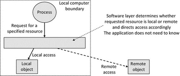
FIGURE 6.1 Generic representation of resource virtualization via a software layer or service.
An example of resource virtualization is Unix's virtual file system (VFS) that transparently differentiates between accesses to local files that are handled by the Unix file system and accesses to remote files that are handled by the Network File System (NFS).
Figure 6.2 shows how the VFS layer provides access transparency. When a request for a file is received, the VFS layer finds where the file is and directs requests for files that are held locally to the local file storage system. Requests for files that are held on other computers are passed to the NFS client program that makes a request for the file to the NFS server on the appropriate remote computer. The file is then retrieved and passed back to the user through the VFS layer, such that the user is shielded from the complexity of what has gone on; hence, they just get access to the file they requested.
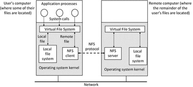
FIGURE 6.2 Access transparency provided by the virtual file system.
6.2.2 Location Transparency
One of the most commonly occurring challenges in distributed systems is the need to be able to locate resources and services when needed. Some desirable capabilities of distributed systems actually increase the complexity of this challenge: such as the ability to replicate resources, the ability to distribute groups of resources so that they are split over several locations, and the ability to dynamically reconfigure systems and services within, for example, to adapt to changes in workload, to accommodate larger numbers of users, or to mask partial failures within the system.
Location transparency is the ability to access objects without the knowledge of their location. A main facilitator of this is to use a resource naming scheme in which the names of resources are location-independent. The user or application should be able to request a resource by its name only, and the system should be able to translate the name into a unique identifier that can then be mapped onto the current location of the resource.
The provision of location transparency is often achieved through the use of special services whose role is to perform a mapping between a resource's name and its address; this is called name resolution. This particular mechanism is explored in detail later in this chapter in the section that discusses name services and the Domain Name System (DNS).
Resource virtualization using a special layer or service (as discussed in “Access transparency”) also provides location transparency. This is because the requesting process does not need to know where the resource is located in the system, it only has to pass a unique identifier to the service, and the service will locate the resource.
Communication mechanisms and protocols that require that the address of the specific destination computer be provided are not location-transparent. Setting up a TCP connection with, or sending a UDP datagram to, a specific destination is clearly not location-transparent (unless the address has been automatically retrieved in advance using an additional service), but nevertheless, the underlying mechanisms of TCP and UDP (when used in its point-to-point mode) are not location-transparent.
Higher-level communication mechanisms such as remote procedure call (RPC) and Remote Method Invocation (RMI) require that the client (the calling process) knows the location of the server object (this is usually supplied as a parameter to the local invocation). Therefore, RPC and RMI are not location-transparent. However, as with socket-level communication discussed above, these mechanisms can be used in location-transparent applications by prefetching the target address using another service such as a name service.
Middleware systems provide a number of forms of transparency including location transparency. The whole purpose of middleware is to facilitate communication between components in distributed systems while hiding the implementation and distribution aspects of the system. This requires built-in mechanisms to locate components on demand (usually based on a system-wide unique identifier) and to pass requests between components in access and location-transparent ways. An object request broker (ORB) is a core component of middleware that automatically maps requests for objects and their methods to the appropriate objects anywhere in the system. Middleware has been introduced in Chapter 5 and is also discussed in further detail later in this chapter.
Group communication mechanisms (discussed later in this chapter) provide a means of sending a message to a group of processes without knowing the identity or location of the individuals and thus provide location transparency.
Multicast communication also permits sending a message to a group of processes, but there are several different implementations. In the case that the recipients are identified collectively by a single virtual address that represents the group, then it is location-transparent. However, in the case where the sender has to identify the individual recipients in the form of a list of specific addresses, it is not location-transparent.
Broadcast communication is inherently location-transparent as it uses a special address that causes a message to be sent to all possible recipients. A group of processes can communicate without having to know the membership of the group (such as the number of processes and the location of each).
6.2.3 Replication Transparency
Distributed systems can comprise many resources and can have many users who need access to those resources. Having a single copy of each resource can be problematic; it can lead to performance bottlenecks if lots of users need to access the same resource and it also leaves the system exposed to the risk of one of the resources becoming unavailable, preventing work being done (e.g., a file becomes corrupted or a service crashes). For these reasons, among others, replication of resources is a commonly used technique.
Replication transparency requires that multiple copies of objects can be created without any effect of the replication seen by applications that use the objects. This implies that it should not be possible for an application to determine the number of replicas or to be able to see the identities of specific replica instances. All copies of a replicated data resource, such as files, should be maintained such that they have the same contents, and thus, any operation applied to one replica must yield the same results as if applied to any other replica. The provision of transparent replication increases availability because the accesses to the resource are spread across the various copies. This is relatively easy to provide for read-only access to resources but is complicated by the need for consistency control where updates to data objects are concerned.
The focus of the following discussion is on the mechanistic aspects of implementing replication. The need for resources to be replicated to achieve nonfunctional requirements in systems, including robustness, availability, and responsiveness, has been discussed in detail in Chapter 5. There is also an activity in that chapter that explores replication in action.
The most significant challenge of implementing replication of data resources is the maintenance of consistency. This must be unconditional; under all possible use scenarios, the data resources must remain consistent. Regardless of what access or update sequence occurs, the system should enforce whatever controls are needed to ensure that all copies of the data remain correct and reflect the same value, such that whichever copy is accessed, the same result is achieved. For example, a pair of seemingly simultaneous accesses to a particular resource (by two different users) may actually be serialized such that one access takes place and completes before the other starts. This should be performed on short timescales so that users do not notice the additional latency of the request and thus have the illusion that they are the only user (see also “Concurrency transparency” for more details).
When one copy of a replicated data resource is updated, it is necessary to propagate the change to the other copies (maintaining consistency as mentioned above) before any further accesses are made to those copies to ensure that out-of-date data are not used and that updates are not lost.
There are several different update strategies that can be used to propagate updates to multiple replicas. The simplest update strategy is to allow write access at only one replica, limiting other replicas to read-only access. Where multiple replicas can be updated, the control becomes more complex; there is a trade-off between the flexibility benefits of allowing multiple replicas to be accessed in a read-write fashion and the additional control and communication overheads of managing the update propagation.
Access to shared resources is usually provided via services. Application processes should not in general access shared resources directly because, in such a case, it is not possible to exercise access control and therefore maintain consistency. Therefore, the replication of data resources generally implies the replication of the service entities that manage the resources. So, for example, if the data content of a database is to be replicated, then there will need to be multiple copies of the database service, through which access to the data is facilitated. Figure 6.3 illustrates some models for server replication and update propagation.
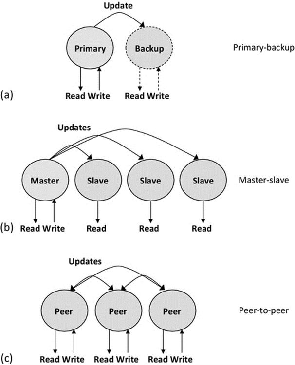
FIGURE 6.3 Some alternative models for server replication.
Figure 6.3 shows three different models for server replication. The most important aspect of these models is the way in which updates are performed after a process external to the service has written new data or updated existing data. The fundamental requirement is that all replicas are just that (exact replicas of each other) a service is inconsistent if the different copies of its data do not hold identical values. Part A of the figure shows the primary-backup model (also called the master-backup model). Here, only the primary instance is visible to external processes, so all accesses (read and write) are performed at the primary, and thus, there can be no inconsistency under normal conditions (i.e., when the primary instance is functioning). Updates performed at the primary instance are propagated to the backup instance at regular periods or possibly immediately each time the primary data are changed. The backup instance is thus a “hot spare”; it has a full copy of the service's data and can be made available to external processes as soon as the primary node fails. The strength of this approach is its simplicity, while it has the weaknesses of only providing one instance of the service at any given time (so is not scalable). There is a small window of opportunity for the two copies to become inconsistent, which can arise if the primary updates its database and then crashes before managing to propagate the update to the backup instance. Primary-backup (master-backup) replication has been explored in detail in activity A3 in Chapter 5.
Figure 6.3 part B shows the master-slave model. All instances of the service can be made available for access by external processes, but write requests are only supported by the master instance and must be propagated to all slave instances as soon as possible so that reads are consistent across the entire service. This replication model is ideal for the large number of applications in which read access is more frequent than write access. For example, in file systems and database systems, reads tend to be more common than writes because updates tend to require a read-modify-write sequence, and thus, writing incorporates a read (the exception being when new files or records, respectively, are created), but reading doesn't incorporate a write. There is no absolute limit to the number of slave instances so the model is very scalable with respect to read requests. A large number of write requests can become a bottleneck because of the requirement to propagate updates, and this becomes more severe as the number of slaves (whose contents must be kept consistent) becomes higher. Mechanisms such as the two-phase commit (see below) should be used to ensure that all updates are either completed (at all nodes) or rolled back to the previous state so that all copies of the data remain consistent even when one instance cannot be updated. In the case of a rollback, the affected update is lost; in which case, the external process that submitted the original request must resubmit it to the service. The slave instances are all potential “hot spares” for the master, should it fail. An election algorithm (see later) is required to ensure that failure of the master is detected and acted upon quickly, selecting exactly one slave to be promoted to master status. The existence of multiple master instances would violate the consistency of the data as multiple writes could occur at the same data record or file at the same time but at different instances, leading to lost updates and inconsistent values held at different nodes.
Figure 6.3 part C shows the peer-to-peer model. This model requires very careful consideration of the semantics of file updates and the way that the data are replicated. It is challenging to implement where global consistency is required at the same time as requiring that each replica has a full copy of the data. This service can however be very useful where the data are fragmented and each node only holds a small subset of the entire data, and thus, the level of replication is lower (i.e., when an update must be performed, it only has to be propagated to the subset of nodes that have copies of the particular data object). This replication model is ideally suited to applications where most of the data are personalized to particular end users, and thus, there is a naturally low level of replication. This approach has become very popular for mobile computing with applications such as file sharing and social networking running on user's portable computing devices such as mobile phones and tablets.
6.2.3.1 Invalidation
Caching of local copies of data within distributed applications is a specialized form of replication to reduce the number of remote access requests to the same data. Caching schemes tend to not update all cached copies when the master copy is updated; this is because of the communication overhead involved, coupled with the possibility that the process holding the cached copy may not actually need to access the data again (so propagating the update would be wasted effort). In such systems, it is still necessary to inform the cache holders that the data they hold are out of date; this is achieved with an invalidation message. In such case, the application only needs to rerequest the data from the master copy if it needs to access the same again.
6.2.3.2 Two-Phase Commit (2PC) Protocol
Updating multiple copies of a resource simultaneously requires that all copies are successfully updated; otherwise, the system will become inconsistent. For example, consider that there are three copies of a variable named X, which has the value 5 initially. An update to change the value to 7 occurs; this requires that all three copies are changed to the value 7. If only two of the values change, the consistency requirement is violated. There could however be reasons why one of the copies cannot be updated: perhaps the network connection has temporarily failed. In such a case where one copy cannot be updated, then none of them should be, once again preserving consistency. In such a situation, the requestor process wanting to perform the update will be informed that the update failed and will be able to resubmit the update later.
The two-phase commit protocol is a well-known technique to ensure that the consistency requirement is met when updating replicas. The first of the two phases determines whether it is possible to update all copies of the resource, and the second phase actually commits the change on an all-or-none basis.
Operation: A commit manager (CM) coordinates a transaction that may involve several participating processes to update replicated data at several sites (see Figure 6.4):
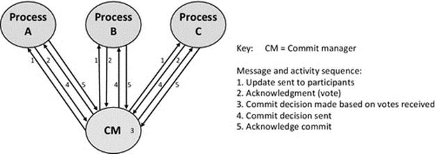
FIGURE 6.4 The two-phase commit protocol.
• Phase 1. An update request is sent to each participating process and each replies with an acknowledgment that they have managed to perform the update (or otherwise that they are not able to). Updates are not made permanent at this stage; a rollback to the original state may be required. The acknowledgments serve as yes or no votes.
• Phase 2. The CM decides whether to commit or abort based on the votes received. If all processes voted yes in phase 1, then a commit decision will be taken; otherwise, the transaction is aborted. The CM then informs participating nodes whether to commit the transaction (i.e., make the changes permanent or rollback).
Figure 6.4 shows the behavior and sequence of messages that constitute the two-phase commit protocol.
The first two messages 1 and 2 represent the first phase of the protocol in which the update is sent to each participating process and they send their votes back (informing of their ability to perform the update). The CM then decides whether or not to commit, based on the votes (step 3). The final two messages 4 and 5 represent the second phase in which the processes are told whether to commit or abort, and each sends back an acknowledgment to confirm their compliance.
6.2.4 Concurrency Transparency
Distributed systems can comprise many shared-access resources and can have many users (and applications running on behalf of users), which use those resources. The behavior of users is naturally asynchronous; this means that they each perform actions when they need to without knowing or checking what others are doing. The resulting asynchronous nature of resource accesses means that there will be occasions where two or more processes attempt to access a particular resource simultaneously.
Concurrency transparency requires that concurrent processes can share objects without interference. This means that the system should provide each user with the illusion that they have exclusive access to the resource.
Concurrent access to data objects raises the issue of data consistency, but from a slightly different angle to that discussed in the context of data replication (above). In the case of replication, there are multiple copies of a resource being updated with the same value, whereas with concurrent access, there are multiple entities updating a single resource. These are different variations of the same fundamental problem and equally important.
In a situation where two or more concurrent processes attempt to access the same resource, there needs to be some regulation of actions. If both processes only read the resource data, then the order of the two reads does not matter. However, if one or both of them write a new value to the resource, then the sequence with which the accesses take place becomes critical to ensuring that data consistency is maintained. Typically, updating a data value follows a read-update-write sequence. If each whole sequence is isolated from other sequences (e.g., by wrapping them inside a transaction mechanism or by locking the resource for the duration of the sequence so that one process has temporary exclusive access), then consistency is preserved. However, where the access sequences of the two processes are allowed to become interleaved, the lost update problem can arise and the system becomes inconsistent (the lost update problem was introduced in Chapter 4 and is discussed further below).
Figure 6.5 illustrates the lost update problem, using an airline booking system as a case example. The application must support multiple concurrent users who are unaware of the existence of other users. The users should be presented with a consistent view of the system, and even more importantly, the underlying data stored in the system must remain consistent at all times. This can be difficult to achieve in highly dynamic applications. For the airline booking application, we consider the consistency requirement that (for a specific flight, on a specific aircraft) the total number of seats available plus the total number of seats booked must always be equal to the total number of seats on the aircraft. It must not be possible for two users to manage to book the same seat or for seats to be “lost,” for example, a seat is booked and then released, but somehow is not added back to the available pool.
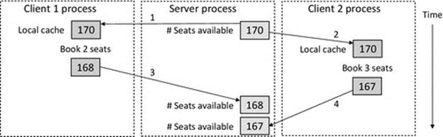
FIGURE 6.5 The lost update problem (illustrated with an airline seat booking scenario).
The scenario shown in Figure 6.5 starts in a consistent state in which there are 170 seats available. In step 1, client1 reads the number of seats available and caches it locally. Soon after this, in step 2, client2 does the same. Imagine that this activity is somehow linked to users browsing an online booking system, taking a while to decide whether to book or not and then submitting their order. Client1 then books 2 seats and writes back the new availability, which is 170 − 2 = 168 (step 3 in the figure). Later, client2 books 3 seats and writes back the new availability, which is 170 − 3 = 167 (step 4). The true availability of seats is now 170 − (2 + 3) = 165. The sequence of accesses in the scenario has led to the creation of two seats in the system that do not actually exist on the plane; therefore, the system is inconsistent.
It is important that you can see where the problem lies in this scenario: it arises because the sequences of accesses of the two clients were allowed to overlap. If client2 had been forced to reread the availability of seats after client1's update, then the system would have remained consistent.
In addition to the consistency aspect of concurrency transparency, there is also a performance aspect. Ideally, user requests can be interleaved on a sufficiently fine-grained timescale that they do not notice a performance penalty arising from the forced serialization occurring behind the scenes. If resources are locked for long periods of time, the concurrency transparency is lost, as users notice that transaction times increase significantly when system load or the number of users increases.
Important design considerations include deciding what must be locked and when and ensuring that locks are released promptly when no longer needed. Also important is the scope of the locking; it is undesirable to lock a whole group of resources when only one item in the group is actually accessed. To put this into context, consider the options for preserving database consistency: locking entire databases during transactions temporarily prevents access to the entire database and is highly undesirable from a concurrency viewpoint. Table-level locking enables different processes to access different tables at the same time, because their updates do not interfere, but still prevents access to the entire locked table even if only a single row is being accessed. Row-level locking is a fine-grained approach that increases transparency by allowing concurrent access at the table level.
6.2.4.1 Transactions
A transaction is an indivisible sequence of related operations that must be processed in its entirety or aborted without making any changes to system state. A transaction must not be partially processed because that could corrupt data resources or lead to inconsistent states.
Transactions were introduced in Chapter 4. Recall that there are four mandatory properties of transactions (the ACID properties):
• Atomicity. The transaction cannot be divided. The whole transaction (all suboperations) is carried out or none of it is carried out.
• Consistency. The stored data in the system must be left in a consistent state at the end of the transaction (this leads on from the all-or-nothing requirement of atomicity). Achieving the requirement of consistency is more complex if the system supports data replication.
• Isolation. There must be no interference between transactions. Some resources need to be locked for the duration of the transaction to ensure this requirement is met. Some code sections need to be protected so that they can only be entered by one process at a time (the protection mechanisms are called MUTEXs because they enforce mutual exclusion).
• Durability. The results of a transaction must be made permanent (stored in some nonvolatile storage).
Figure 6.6 relates together the four properties of transactions in the context of a multipart transaction in which partial results are generated but must not be made visible to processes outside of the transaction.
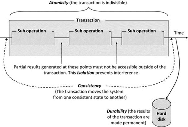
FIGURE 6.6 The four properties of transactions.
The transaction properties are placed into the perspective of a banking application example:
The banking application maintains a variety of different types of data, in a number of databases. These data could include customer accounts data, financial products data (e.g., the rules for opening different types of accounts and depositing and withdrawal of funds), interest rates applicable, and tax rates applicable. A variety of different transactions can occur, depending on circumstances. Transaction types could include open new account, deposit funds, withdraw funds, add net interest, generate annual interest and tax statement, and close account. Each of these transactions may be internally subdivided into a number of steps and may need to access one or more of the databases.
Consider a specific transaction type: add net interest. This transaction may need to perform the following steps: (1) read the account balance and multiply by the current gross interest rate to determine the gross interest amount payable; (2) multiply the gross interest amount by the tax rate to determine the tax payable on the interest; (3) subtract the tax payable from the gross interest amount to determine the net interest payable.
Prior to the transaction, the system is in a consistent state and the following three values are stored (in three separate databases): account balance = £1000; interest rate = 2%; tax rate = 20%. Figure 6.7 illustrates the internal operation of the transaction.
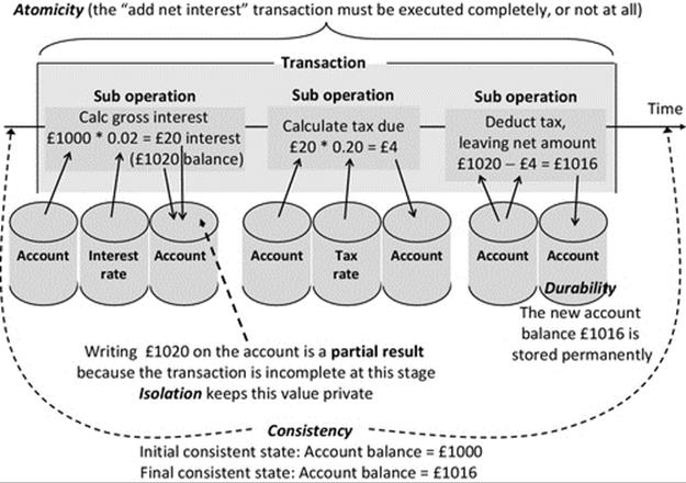
FIGURE 6.7 The internal operation of the “add net interest” transaction of the banking application.
Figure 6.7 places the ACID transaction properties into the perspective of the mechanics of the banking application transaction. The transaction operates in three steps leading to temporary internal states (partial results), which must not be visible externally. When the transaction completes, the system is in a new consistent state, the account balance having been updated to the value £1016.
The isolation property of transactions is particularly important with respect to concurrency transparency because it prevents external processes accessing partial results generated temporarily as a transaction progresses. In the example illustrated in Figure 6.7, a temporary value of £1020 is written to the account, but the transaction is only partially complete at this stage, and tax is yet to be deducted. Therefore, the user never actually has that amount to withdraw. If the value were exposed to other processes, then the system could become inconsistent. If the user were to check their balance in the short time window while the temporary value was showing on the account, they would think they had more money than they actually do have. Worse still would be if the user were allowed to withdraw £1020 at this point because they do not actually have that much money in the account. When the transaction finally completes, the system is left in a consistent state with £1016 in the account; this value can now be exposed to other processes.
A further example is provided by re-presenting the airline seat booking system (seen earlier in this section) as a series of transactions. The forced serialization (and thus isolation) overcomes the inconsistency weakness of the earlier design.
Figure 6.8 presents a transaction implementation of the airline seat booking system. This approach serializes the two seat booking operations that would lead to an inconsistent state if allowed to become interleaved. The system is left in a consistent state after each transaction, in which the number of seats available and the number of seats booked always are equal to the total number of seats on the aircraft.
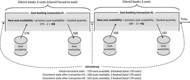
FIGURE 6.8 A transaction implementation of the airline seat booking system.
6.2.5 Migration Transparency
Distributed systems tend to be dynamic in a number of ways including changes in the user population and the activities they carry out, which in turn leads to load-level fluctuations on different services at various times. Systems are also dynamic due to the addition and relocation of physical computers, continuous changes in network traffic levels, and the random failure of computers and network connections.
Due to the dynamic nature of these systems, it is necessary to be able to reconfigure the resources within the system, for example, to relocate a particular data resource or service from one computer to another.
Migration transparency requires that data objects can be moved without affecting the operation of applications that use those objects and that processes can be moved without affecting their operations or results.
In the case of migration of data objects (such as files) in active use, access requests from processes using the object must be transparently redirected to the object's new location. Where objects are moved between accesses, techniques used to implement location transparency can suffice. A name service (discussed later) provides the current location of a resource; its history of movement is of no consequence as long as its current location after moving is known. However, there is a challenge in keeping the name service itself up to date if resources are moved frequently.
Process transfers can be achieved preemptively or nonpreemptively. Preemptive transfers involve moving a process in midexecution. This is complex because the process' execution state and environment must be preserved during the transfer. Nonpreemptive transfers are done before the task starts to execute so the transfer is much simpler to achieve.
6.2.6 Failure Transparency
Failures in distributed systems are inevitable. There can be large numbers of hardware and software components interacting, dependent on the communication links between them. The set of possible configurations and behaviors that can arise is too great in general that every scenario can be tested for; therefore, there will always be the possibility of some unforeseen combination of circumstances that leads to failure. In addition to any built-in reliability weaknesses they may have, hardware devices and network links can fail due to external factors; for example, a power cut may occur or a cable is accidentally unplugged.
While it is not possible to prevent failures outright, measures should be taken to minimize the probability of failures occurring and to limit the consequences of failures when they do happen.
Good system-level design should take into account the reality that any component can fail and should avoid having critical single points of failure where possible. Software design should avoid unnecessary complexity within components and in the connectivity with, and thus dependency upon, other components (see the section on component coupling in Chapter 5). Additional complexity increases the opportunities for failure; and the more complex the system, the harder it is to test. This leads to undertesting where not all of the functional and behavioral scope is covered by tests. Even where testing is thorough, it cannot prove that a failure will not take place. Latent faults are present in most software systems. These are faults that have not yet shown up; faults in this category often only occur in a particular sequence or combination of events so they can lurk undetected for a long time.
Once we have exhausted all possible design-time ways to build our systems to be as reliable as possible, we need to rely on runtime techniques that will deal with the residual failures that can occur.
Failure transparency requires that faults are concealed so that applications can continue to function without any impact on behavior or correctness. Failure transparency is a significant challenge! As mentioned above, many different types of fault can occur in a distributed system.
Communication protocols provide a good example of how different levels of runtime failure transparency can be built in through clever design. For example, compare the TCP and UDP. TCP has a number of built-in features including sequence numbers, acknowledgments, and a retransmission-on-time-out mechanism that transparently deal with various issues that occur at the message transmission level, such as message loss, message corruption, and acknowledgment loss. UDP is a more lightweight protocol and, as a result, has none of these facilities and, hence, is commonly referred to as a “send and pray” protocol.
6.2.6.1 Support for Failure Transparency
A popular technique to provide a high degree of failure transparency is to replicate processes or data resources at several computing hosts, thus avoiding the occurrence of a single point of failure (see “Replication transparency”).
Election algorithms can be used to mask the failure of critical or centralized components. This approach is popular in services that need a coordinator and can include replicated services in which one copy is allocated the role of master or coordinator. On the failure of the coordinator, another service member process will be elected to take over the role. Election algorithms are explored in detail later in this chapter.
In all replicated services or situations where a new coordinator is elected when a failure occurs, the extent to which the original failure is masked is dependent on the internal design of the service, in particular the way in which state is managed. The new coordinator may not have a perfect copy of the state information that the previous one had (e.g., an instantaneous crash can occur during a transaction), so the system may not be in an identical situation after recovery. This scenario should be given careful consideration during the design effort to maximize the likelihood that the system does remain entirely consistent across the handover. In particular, the use of stateless server design can reduce or remove the risk of state loss on server failure, as all state is held on the client side of connections (see the discussion on stateful versus stateless services in Chapter 5).
Even when stateless services are used, problems can still arise. For example, if a single requested action is carried out multiple times at a server, the correctness or consistency of the system could be disrupted. Consider, for example, in a banking application, the function “Add annual interest” being executed multiple times by accident. This could happen where a request is sent and not acknowledged; the client may resend the message on the assumption that the original request was lost, but in fact, the message had arrived and it was actually the acknowledgment that was lost; the outcome being that the server will receive two copies of the request. One way to resolve this is to use sequence numbers so that duplicate requests can be identified. Another approach is to design all actions to be idempotent.
An idempotent action is one that is repeatable without having side effects. The use of idempotent requests contributes to failure transparency because it hides the fact that a request has been repeated, such that the intended outcome is correct. There is no side effect of requesting the action more than once, whether the action is actually carried out multiple times or not. Another way to think of this is that the use of idempotent actions allows certain types of fault to occur while preventing them from having any impact and therefore removing the need to handle the faults or recover from them.
Generic request types that can be idempotent include “set value to x,” “get value of item whose ID is x,” and “delete item whose ID is x.”
Generic request types that are not idempotent include “add value y to value x,” “get next item,” and “delete item at position z in the list.”
A specific example of a nonidempotent action is “add 10 pounds to account number 123.” This is because (if we assume the initial balance is 200 pounds) after being executed once, the new balance will be 210 pounds, and after two executions, the balance will be 220 pounds and so on.
However, the action can be reconstructed as a series of two idempotent actions, each of which can be repeated without corrupting the system's data. The first of the new actions is “get account balance,” which copies the balance from the server side to the client side. The result of this is that the client is informed that the balance is 200 pounds. If this request is repeated multiple times, the client is informed of the balance value several times, but it is still 200 pounds. Once the client has the balance, it then locally adds 10 pounds. The second idempotent action is “set account balance to 210 pounds.” If this action is performed once or more times in succession, the balance at the server will always end up at 210 pounds. In addition to being robust, the approach of shifting the computation into the client further improves the scalability of the stateless server approach. However, this technique is mostly useful for nonshared data, such as the situation in the example above in which each client is likely to be interested in a unique bank account. Where the data are shared, as in the earlier airline seat booking example, transactions (which are more heavyweight and less scalable) are more appropriate due to the need for consistency across multiple actions and the need to serialize accesses to the system data.
Idempotent actions are also very useful in safety-critical systems, as well as in systems that have unreliable communication links or very high latency communication. This is because the role of acknowledgments is less critical when idempotent requests are used and the not uncommon problem of the time-out being too short (causing retransmission) does not result in erroneous behavior at the application level.
Checkpointing is an approach to fault tolerance that can be used to protect from the failure of critical processes or from failure of the physical computers that critical processes run on.
Checkpointing is the mechanism of making a copy of the process' state at regular intervals and sending that state to a remote store (the state information that is stored includes the process' memory image, such as the value of variables, as well as process management details such as which instruction is to be executed next, and IO details such as which files are open and what communication links are set up with other processes.
If a checkpointed process crashes or its host computer fails, then a new copy of the process can be restarted using the stored state image. The new process begins operating from the point the previous one was at when the last checkpoint was taken. This technique is particularly valuable for protecting the work performed by long-running processes such as occur in scientific computing and simulations such as weather forecasts that may run for many hours. Without checkpointing, a failed process would have to start again from the beginning, potentially causing the loss of a lot of work and causing delay to the user who is waiting for the result.
6.2.7 Scaling Transparency
For distributed systems in general, as the system is scaled up, a point is eventually reached where the performance will begin to drop; this could be noticed, for example, in terms of slower response times or service requests timing-out. Small increases in scale beyond this point can have severe effects on performance.
Scaling transparency requires that it should be possible to scale up an application, service, or system without changing the system structure or algorithms. Scaling transparency is largely dependent on efficient design, in terms of the use of resources, and especially in terms of the intensity of communication.
Centralized components are often problematic for scalability. These can become performance bottlenecks as the number of clients or service requests increases. Centralized data structures grow with system size, eventually causing scaling problems in terms of the size of the data and the increased time taken to search the larger structure, impacting on service response times. A backlog of requests can build up rapidly once a certain size threshold is exceeded.
Distributed services avoid the bottleneck pitfalls of centralization but represent a trade-off in terms of higher total communication requirements. This is because in addition to the external communication between clients and the service, there is also the service-internal communication necessary to coordinate the service and, for example, to propagate updates between server instances.
Hierarchical design improves scalability; a very good example of this is the DNS that is discussed in detail later in this chapter. Decoupling of components also improves scalability. Publish-subscribe event notification services (also discussed later) are an example technique by which the extent of coupling and also the communication intensity can be significantly reduced.
6.2.7.1 Communication Intensity: Impact on Scalability
Interaction complexity is a measure of the number of communication relationships within a group of components. Because systems scale can change, interaction complexity is described in terms of the proportion of the other components in the system each component communicates with, rather than absolute numbers (see Table 6.1).
Table 6.1
Example Interaction Complexities for a System of N Components
|
Typical proportion of other components that each of the N components communicates with |
Interaction complexity |
Typical interpretation |
|
1 |
O(N) |
Each component communicates with another component. This is highly scalable as the communication intensity increases linearly as the system size increases |
|
2 |
O(2N) |
Each component communicates with two other components. Communication intensity increases linearly as the system size increases |
|
N/2 |
O(N2/2) |
Each component communicates with approximately half of the system. This represents an exponential rate of increase of communication intensity and thus can impact on scalability |
|
N − 1 |
O(N2 − N) also written O(N(N − 1)) |
Each component communicates with most or all. This is a steep exponential relationship and can severely impact on scalability |
Communication intensity is the amount of communication that actually occurs, which results from the interaction complexity combined with the actual frequency of sending messages between communicating components and the size of those messages. This is a significant factor that limits the scalability of many systems. This is because the communication bandwidth is finite in any system and the communication channels become bottlenecks as the amount of communication builds up. Communication is also relatively time-consuming compared with computation. As the ratio of time spent communicating (including waiting to communicate due to network congestion and access latency) to computation time increases, the throughput and efficiency of systems fall. The reduction in performance eventually becomes a limiting factor on usability. If the performance cannot be restored by adding more resource while leaving the design unchanged, then the design is said to be not scalable or to have reached the limit of its scalability.
Some diverse examples of interaction complexity are provided below:
• The bully election algorithm in its worst-case scenario during an election has O(N2 − N) interaction complexity (the bully election algorithm is discussed in “Election algorithms” later in this chapter).
• A peer-to-peer media sharing application (as explored in activity A2 in Chapter 5) may have typical interaction complexity of between O(2N) and O(N2/2) depending on the actual proportion of other peers that each one connects to.
• The case study game that has been used as a common point of reference throughout the book has a very low interaction complexity. Each client connects to one server component regardless of the size of the system, so system-wide interaction complexity is O(N) where N is the number of clients in the system.
Figure 6.9 shows two different interaction mappings between the components of similar systems. Part A illustrates a low-intensity mapping in which each component connects with on average one other, so the interaction complexity is O(N). In contrast, part B shows a system of highly coupled components in which each component communicates with approximately half of the others, so the interaction complexity is O(N2/2).
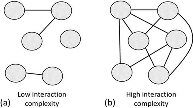
FIGURE 6.9 Illustration of low and high interaction complexity.
Figure 6.10 provides a graphic illustration of the way in which interaction complexity affects the relationship between the size of the system (the number of components) and the resulting intensity of communication (the number of interaction relationships). The steepness of the curves associated with the more intense interaction complexities illustrates the relative severity of their effect on scalability.
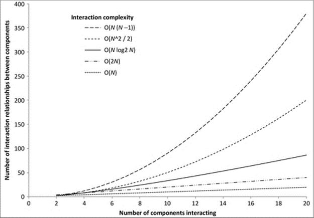
FIGURE 6.10 The effect of various interaction complexities on the relationship between the size of the system and the resulting intensity of communication.
6.2.8 Performance Transparency
The performance of distributed systems is affected by numerous aspects of their configuration and use.
Performance transparency requires that the performance of systems should degrade gracefully as the load on the system increases. Consistency of performance is a significant aspect of the user experience and can be more important than absolute performance. A system that has consistent good performance is better received than one in which the performance is outstanding some of the time but can degrade rapidly and unpredictably, which leads to user frustration. Ultimately, this is a measure of usability.
6.2.8.1 Support for Performance Transparency
Performance (an attribute of the system) and performance transparency (a requirement on performance) are affected by the design of every component in the system and also by the collective behavior of the system that itself cannot be predicted by knowing the behavior of each individual component, due to the complex runtime relationships and sequences of events that occur.
High performance cannot therefore be guaranteed through the implementation of any particular mechanism; rather, it is an emergent characteristic that arises through consistently good design technique across all aspects of the system. Performance transparency is an explicit goal of load-sharing schemes that attempt to evenly distribute the processing load across the processing resources so as to maintain responsiveness.
6.2.9 Distribution Transparency
Distribution transparency requires that all details of the network and the physical separation of components are hidden such that application components operate as though they are all local to each other (i.e., running on the same computer) and therefore do not need to be concerned with network connections and addresses.
A good example is provided by middleware. A virtual layer is created across the system that decouples processes from their underlying platforms. All communication between processes passes through the middleware in access-transparent and location-transparent ways, providing the overall effect of hiding the network and the distribution of the components.
6.2.10 Implementation Transparency
Implementation transparency means hiding the details of the ways in which components are implemented. For example, this can include enabling applications to comprise components developed in different languages; in which case, it is necessary to ensure that the semantics of communication, such as in method calls, are preserved when these components interoperate.
Middleware such as CORBA provides implementation transparency. It uses a special interface definition language (IDL) that represents method calls in a programming language-neutral way such that the semantics of the method call between a pair of components are preserved (including the number parameters and data type of each parameter value and the direction of each parameter, i.e, being passed into the method or returned from the method) regardless of the combination of languages the two components are written in.
6.3 Common Services
Distributed applications have a number of common requirements that arise specifically because of their distributed nature and of the dynamic nature of the system and platforms they operate on. Common requirements of distributed applications include
• an automatic means of locating services and resources,
• an automatic means of synchronizing clocks,
• an automatic means of selecting a coordinator process from a group of candidates,
• mechanisms for the management of distributed transactions to ensure consistency is maintained,
• communications support for components operating in groups,
• mechanisms to support indirect and loose coupling of components to improve scalability and robustness.
It is therefore sensible that a group of support services are provided generically in systems, which provide services to applications in standard ways. Application developers can integrate calls to these services into their applications instead of having to implement additional functionality within each application. This saves a lot of duplicated effort that would be costly, would significantly extend lead times, and could ultimately reduce quality as each developer would implement different variations of services leading to possible inconsistency.
In addition to specific functionalities such as those mentioned above, common services also contribute to the provision of all transparency forms discussed earlier in this chapter and also to the nonfunctional requirements of distributed applications discussed inChapter 5.
Common services are generally regarded as an integral part of a distributed systems infrastructure and are invisible to users. These support services are usually distributed or replicated across the computers in the system and therefore have the same quality requirements (robustness, scalability, responsiveness, etc.) as the distributed applications themselves. Some of the common services are exemplars of good distributed application design; DNS is a particular example.
There are a wide range of possible services and mechanisms that can be considered in the common services category, so this chapter focuses on some of the most significant and frequently used services. The common services and mechanisms explored in the following sections of this chapter are
• name services and directory services,
• the DNS (a very important example of a name service, treated in-depth),
• time services,
• clock synchronization mechanisms,
• election algorithms,
• group communication mechanisms,
• event notification services,
• middleware.
6.4 Name Services
One of the biggest challenges in a distributed system is finding resources. The very fact that the resources are distributed across many different computers means that there needs to be a way to automatically find the resources needed and to be able to do this very quickly and reliably.
Consider the situation where one software component needs to find the location of another, so that a message can be sent to it. Keeping at the very highest level, there are only two approaches: Information that is already known is used and there is a way to look up the information needed on demand. There are several parallels with the way people find resources: two good examples are phone numbers and Web sites. You probably know the phone numbers and Web site addresses that you use regularly. These are memorized, so this is the equivalent of built-in or hard-coded, if you were a software component. One pertinent issue here is that if one of your friends changed their number, then your memorized data are of no use and you would need a way to get hold of the new number and then rememorize it. For the phone numbers and Web sites that you cannot remember, which realistically is most of them, you need some way to be able to find them; you need a service that searches for them based on a description. Your mobile phone has a database built into it, into which you can store your regularly needed phone numbers, using the name of the phone number owner as a key. You then type in the person's name when you need to phone them (you don't need to remember the number), the database is searched, and the phone number is retrieved; this is essentially a simple form of name service (more specifically, this is an example of a directory service; see discussion below).
Consider the number of resources in a system as large as the Internet. There are thousands of millions of computers connected to the Internet. There are hundreds of millions of Web sites and some of these Web sites have hundreds of pages. The numbers are staggering, but how many can you remember? You probably don't remember very many at all, but you have ways to find out, using services that you probably use many times a day without necessarily thinking about how they operate.
To illustrate, let me set you a typical day-to-day information-retrieval task (try to do this right away without thinking too much about it): find the Web site for your local government office (such as your local council) where you would get information about local services such as weekly rubbish collections.
Did you manage to get the Web site displayed on your computer? If so, then I expect you probably used two different services. Firstly, you probably used a search engine (such as Bing, Google, and Yahoo), where you submitted a textual query such as “Havering council services” and were presented with a number of uniform resource locators (URLs; these were introduced in Chapter 4). The results I get after this first stage include those shown in Figure 6.11.
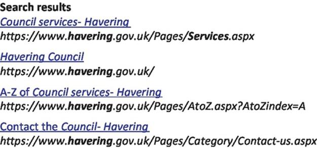
FIGURE 6.11 The first four results returned by the search engine, for my search string.
The next step requires you to choose one of the search results that appears to describe the Web site that you are actually looking for and to click on the provided hyperlink (these are the underlined sections of text, and when clicked, the associated Web page will automatically be opened in a browser). Modern search engines are very good at contextually ordering the results of the search, and in this particular case, the first result in the list does seem the most promising, so I would now click on the first link in the list.
This is the point where the second service (a name service) comes into play, and because you are using it automatically, it is quite possible that you are not even aware that you are using it. Several things must happen in sequence, in order to display the Web page. First, the URL must be converted to an IP address (the address of the host computer where the relevant Web server is located), and then, a TCP connection can be made to the Web server. Once the TCP connection is set up, then a request for the Web page can be sent to the Web server, and the Web page contents are sent back to my computer. Finally, the Web page is displayed on my screen. The name service is the part of the system that converts the URL into the IP address of the Web server's host computer's address. The actual name service used in the Internet is the DNS, which is discussed in detail later in this chapter.
6.4.1 Name Service Operation
A name service is a network service that translates one form of address into another. A very common requirement is to translate a human-meaningful address type, such as a URL, into the type of address used to actually communicate with components within a system (such as an IP address).
The fundamental need for name services stems from several factors:
• Networks can be huge, containing many computers, and the IP addresses of computers are logical, not physical. This means that a computer's IP address is related to its logical connection into the network. If the computer is moved to a different subnet, then its IP address will change; this is a necessity for routing to operate correctly (see the discussion in Chapter 4).
• Distributed applications can span across many physical computers. The configuration of the application can change, such that different components are located on different computers at different times.
• Networks and distributed systems are dynamic; resources are added, removed, and moved around. Even if you know where all of the resources are at one point in time, your list can be out of date soon after.
• The means to locate resources needs to be standardized for a particular system and externalized from the application software components. It is not desirable to have to embed special mechanisms into each component separately as this represents a lot of effort (design and also testing) and increases the complexity of components significantly.
A fundamental part of name service functionality is to look up the name of a resource (which has been provided in a request message) in a database and to extract the corresponding address details. The address details are then sent back to the requestor process, which uses the information to access the resource. This subset of name service functionality can be described as a directory service (which is discussed in more detail later).
A name service is differentiated from a directory service by the additional functionality and transparency it provides. A name service implements a namespace, which is a structured way to represent resource names. To achieve scalability, a hierarchical namespace is necessary in which a resource name explicitly maps onto its position in the namespace and thus assists in locating the resource (see the discussion on hierarchical addressing in Chapter 3).
In the context of name services, the most important example of hierarchical names is URLs, in which the structure of the resource name relates to its logical location. Consider your e-mail address as a simple example. The URL might have the format: A.Student@myUniversity.Academic.MyCountry. This achieves three important requirements. Firstly, it represents the resource, your e-mail inbox, in a human-friendly way so that people can describe it easily and hopefully remember it. Secondly, it contains an unambiguous mapping of the resource (the e-mail inbox named A.Student) to the e-mail server that hosts the resource, which has the logical address myUniversity.Academic.MyCountry. Thirdly, it is globally unique as there are no other e-mail addresses the same as your one anywhere in the world.
A name service may need to be distributed to enhance scalability and to achieve performance transparency by spreading the namespace, and the work of resolving names within the namespace, across multiple servers. To achieve failure transparency, the name service may also need to be replicated, so that there is no single critical instance of the service (i.e., so that each name can be resolved by more than one service instance).
6.4.2 Directory Service
As explained above, a directory service provides a subset of name service functionality; it looks up resources in a directory and returns the result. It does not implement its own namespace, and the directory structure is usually flat rather than hierarchical.
Figure 6.12 illustrates how a directory service is used. The application client passes the name of the required application server to the directory server, which responds with the details stored in its database. A directory service is suitable for use within specific applications or for local resource address resolution in small-scale systems; in which case, the size and complexity of the database storage and lookup are limited.
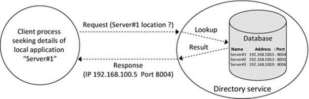
FIGURE 6.12 Overview of directory service operation.
Figure 6.13 shows how a name service wraps a more sophisticated service around the core directory service functionality. In particular, the name service implements a hierarchical namespace and distributes the resource details logically across different directory instances based on the logical position of those resources in the namespace.
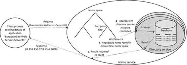
FIGURE 6.13 A directory service as a subcomponent of a name service.
Activity D1 uses the directory service that is integrated into the Distributed Systems Workbench to investigate the need for, and behavior of, name and directory services. The directory service has been designed to work in local, small-scale systems, and therefore, it does not support replication and is not distributed, features you would expect in a scalable and robust name service. Significantly, as the directory service operates locally with a limited number of application servers, it stores their names in a flat addressing scheme, that is, it only uses a single-layer textual name such as “server1” or “AuthenticationServer.”
Figure 6.14 shows the basic interaction between application components and the directory service, as will be explored in activity D1. The client of an application does not initially know the location of its service counterpart so it passes the name of the required service to the directory service (step 1 in the figure). The directory service looks up the application server name and returns its address if found (step 2 in the figure). Once the client has got the server address, it can make a connection in the usual way (steps 3 and 4 in the figure).
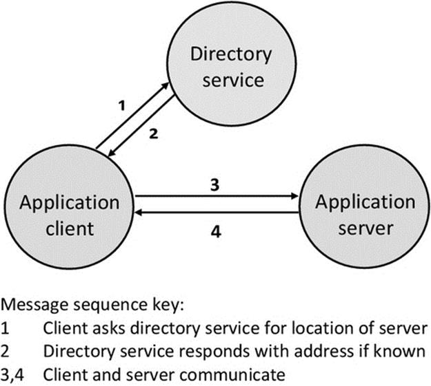
FIGURE 6.14 Basic interaction with the directory service.
Activity D1
Experimentation with a Directory Service
This activity uses the directory service that is integrated into the Distributed Systems Workbench to investigate the need for, and behavior of, name and directory services.
The directory service runs as a process on one of the computers in the local network. Application servers can be registered with the directory service when they are initiated. When a client process needs to access a particular application server, it can request the address details from the directory service, identifying the application server by its textual name. The directory service returns the IP address and port number that the client process needs in order to connect to the application service.
Note that name services and directory services perform essentially the same function, namely, to resolve the name of a resource into its location details that can be used to access the resource. The particular service used in this activity is classified as a directory service. It maintains a database of resources that have registered with it, and upon request, it searches the database for the supplied name and returns to the requestor the relevant location details. The simple directory service demonstrates the essential behavior of a name service without implementing a namespace and without itself being distributed; hence, it has not only limited scalability but also limited complexity. Such a service is ideally suited to automatic resource discovery in small-scale local network systems, but is not appropriate for large-scale systems. The low complexity of the directory service makes it ideal for exploring the fundamental mechanism of resource location.
Prerequisites: Copy the support materials required by this activity onto your computer (see activity I1 in Chapter 1).
Learning Outcomes
1. To gain an appreciation of the need for name/directory services
2. To gain an understanding of the operation of an example directory service
3. To gain an appreciation of the transparency benefits of name/directory services
4. To investigate problem scenarios for the use of directory services
5. To explore service autoregistration with a directory service
This activity uses the set of programs found under the “Directory Service” drop-down in the Distributed Systems Workbench top-level menu. The programs include a directory service, four application servers, and an application client. All of the components can be run on a single computer to get a basic idea of the way the directory service operates, but the activity is best performed in a network of at least three different computers if possible, so that the application servers have different IP addresses and separate the client process from the various server processes it connects to in order to make the experimental scenarios realistic.
Method Part a: Understanding the Need for Name or Directory Services
In this part of the activity, you will run the application client on one computer and the Application Server1 on another. Do not start the directory server on any computer at this stage.
Part A1. Start Server1 on one computer. Directory Service → Application Server1, and then, click “Start server.”
Part A2. Start the client on a second computer (ideally, but, otherwise, you can use the same computer for both client and server). Directory Service → Client.
Note that the client sets a default address for the server to be the same as its own address and sets a default port number of 8000. Even if the address is correct (i.e., you have started the server on the same computer as the client), the port number is wrong. Try sending a request string to the server with these settings (place some text in the “Message to send” box and press the Send button); it should not do anything.
Part A3. Manually configure the client (enter the correct server address and server port details) so that it can communicate with server1 (confirm that the client and server are actually communicating by sending a request string; the server should send back a reversed-order copy of whatever string you typed).
Part A4. Repeat parts A2 and A3 using server2 on a third computer (ideally, otherwise, use the same computer as earlier).
Part A5. Repeat 1.2 and 1.3 using server3 on a fourth computer (ideally, otherwise, use the same computer as earlier).
Expected Outcome for Part A
By now, you should be able to comment on the suitability (especially in terms of the low usability) of this manual client-server binding approach for commercial distributed systems. Try to identify alternative ways that the client could use to locate the required application server.
The screenshots below show the client, on a computer with IP address 192.168.0.2, manually configured to connect to server3, which is on a computer with IP address 192.168.0.3, using port 8006. Note that the “Server required” field is not used at this stage.
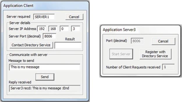
Method Part B: Using the Directory Service
Part B1. Start the directory server on one computer only. Note that the directory service does not support replication. If multiple copies of the directory service exist, they will all respond to a client request; this will confuse the results of the experiment.
Part B2. Run the application client on a second computer (if available) and run the application server1 on a third computer.
Part B2. Press the button on server1 to register the server with the directory server. Observe the directory service information boxes.
Part B4. Use the directory service (the client has a button labeled “Contact Directory Service”) to get server1's address and port details). Observe the “Server details” boxes in the client and the directory server information boxes.
Part B5. Start sever2 and server3 also (on any of the computers available). Register these with the directory service. Contact all three services in sequence, using the client. Each time you wish use a new service, change the name of the service in the “Server required” text box on the client, and then, use the Contact Directory Service button to get the details.
Expected Outcome for Part B
You should now be able to see the benefit of having an automatic name resolution service (as provided by the directory service) to facilitate automated component-to-component binding using only textual component names.
The set of screenshots below shows the system configuration once all of the steps of part B of the activity have been completed. The client and server2 (shown of the left below) were running on a computer with IP address 192.168.0.2, while the directory server and application server1 and server3 (shown on the right below) were running on a computer with IP address 192.168.0.3.
The three application servers have been started and have been registered with the directory service, as can be seen in the “Directory Database” listing within the directory server dialog box. The client has requested the address and port details for each server in turn, from the directory service, as can be seen in the “Request History” listing within the directory server dialog box.
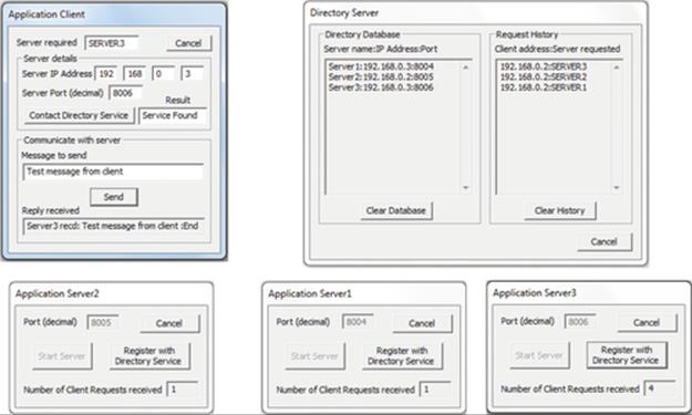
Method Part C: Investigate the Impact of Problem Scenarios on the Behavior of the Directory Service
For this part of the activity, you are encouraged to carry out your own experiments to investigate what happens under a range of scenarios that include the following:
• An application server is not registered when the client asks for its details.
• An application server was registered but has crashed since then.
• An application server was registered at one location but has since been relocated.
• The directory service is running on two different computers simultaneously.
• The directory service is not running at all.
• The directory service crashes after application servers have registered and is then restarted.
Expected Outcome for Part C
Some of the problem scenarios will reveal limitations of the quite simple design of the example directory service. For any problems you discover, repeat experiments to make sure you appreciate the mechanism of the problem (i.e., what is the actual cause of the problem behavior and how/why does it affect the overall system behavior). Identify any modifications that you think might solve the problem.
The screenshot below shows the “Not Found” response from the directory service when the client requests details of an application server that is not registered.
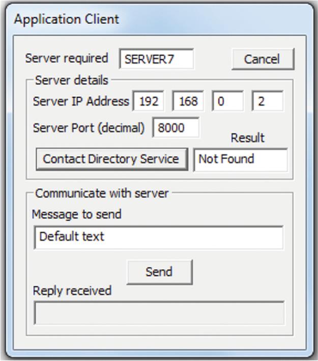
Method Part D: Investigate Service Registration
The problem scenarios identified in part C above do occur in real systems: Application services get relocated within systems, and directory services can crash and recover (with possibly out-of-date information). This means that manually registering services or one-off automated service registration is insufficient in terms of continuously meeting nonfunctional requirements such as usability, robustness, and responsiveness.
Part D1. To appreciate the problem, repeat part C above and move a service (any of application server1, server2, or server3) AFTER you have registered it. Note that the directory service now provides incorrect details. Alternatively shutdown and restart the directory service AFTER an application had registered; the directory service is stateless and thus (after restarting) does not know about the previously registered server.
Part D2. Repeat part D1, but this time, use application server4 (instead of server1, server2, or server3). Notice that there is no button to register the application server with the directory service because it is self-registering. Move server4 as many times as you like. Restart the directory service too. Each time you change something, wait a few seconds and then see if the client can get the server4 details from the directory server.
Expected Outcome for Part D
From your experiments, you should have noticed some distinctly different behavior when using application server4 than when using the other ones.
Question 1. What differences do you notice with respect to server registration?
Question 2. How is the directory service updated?
Question 3. To what extent are the problem scenarios identified in section C overcome?
Question 4. How appropriate is this behavior for large-scale distributed systems?
Reflection
From carrying out this activity, you should have a basic understanding of the behavior of the directory service and appreciate that it is very powerful in terms of transparency and usability. Once the application servers have registered with the directory service, the user only needs to know the textual name of the service they require in order to contact and use the service. Even this aspect could be automated where it is implicitly known, such that the client automatically requests the service it needs, by name upon start-up. In addition to the significant usability benefits, this also achieves location and migration transparency.
Further Investigation
How does the client locate the directory service itself? You may have already worked this out from the experiments you have done, but if not, try a few further experiments to determine it. Try placing the directory server on the same computer as the application servers and on different ones and also investigate having the client process on the same computer as the directory server and on a different one. Here is a clue: do you ever have to provide the address of the directory server?
6.4.3 Challenges of Name Service Design and Implementation
A name service has many of the common nonfunctional design requirements of distributed applications that were identified and discussed in Chapter 5. In particular, the following apply: robustness (because applications rely on the name service for their own operation, any failures will have a ripple effect across other parts of the system; scalability (the name service must be able to scale to meet the needs of the host system and should not become a limiting factor as the system grows; responsiveness, (name resolution is one of the many steps in application execution, and the latency added by the name service should be as low as possible.
In addition to the nonfunctional requirements, there are a number of specific challenges associated with the design, implementation, and use of name services, which affect the correctness of the data held within the service itself, as well as the robustness and scalability of the service. Some of these challenges have been revealed during activity D1.
Server registration: When should application servers register with the name service? Should one-off registration be performed automatically when a service is started? Or should it be performed periodically (to protect against the situation where the name server crashes and restarts, losing details of previous registrations)? If registration is periodic, then how frequently should it occur? (There is a trade-off between the communications cost of doing it too frequently and the latency of the service being updated if the interval between registration events is too long).
Server deregistration: Should application servers deregister as part of their shutdown procedure? If so, what happens if they crash without shutting down correctly? (This will lead to out-of-date information being held by the name service, which will still think the application is present and will continue to advertise it). Could the lack of periodic reregistration activity be used as an automatic indicator that the application is no longer running?
Relocation of application servers: How is the name service updated if an application server is moved? (In many systems, it will be adequate to use an existing deregistration facility prior to the move and then reregister the application after the move.)
The name service's interaction with replicated application servers: If there are many instances of the same application service present, how does the name service determine which instance to direct client requests to? Some possibilities include round-robin, always returning the first instance found in the database, or implementing some form of load-sharing scheme.
Client caching of lookup results: Should application clients cache lookup results, or should they query the name service every time? There is a trade-off between always getting the latest information from the name server (at the cost of higher communication and more work for the name service) and using cached information that could be out of date (in which case, the client may waste time trying to contact an application server at the wrong location). This trade-off needs to be managed based on the extent of dynamism in the system; more static systems are better suited to longer caching periods.
What happens if the directory service crashes: Name services are a vital link in establishing communication within applications and facilitating access to remote resources. The extent to which a system can continue to operate while the name service is down depends on a number of factors that include the frequency with which new connections are made between application components (connections already established are not affected by failure of the name service); whether clients' cache lookup results (in which case they don't always need to contact the name service when establishing connections with application components); and the likelihood that components connect to the same set of other components or different ones each time (thus impacting on the usefulness of the cache contents).
Replication of the name service: Replication can be used to improve the robustness and scalability of a name service. However, if two independent copies of the name service coexist without some form of control or delegation in place, then client requests might be answered by both instances leading to unpredictable behavior, especially if the data held at the two name server instances become inconsistent.
Locating the name service: How do clients find the name service itself? If a name service is needed to find resources and the name service is itself a resource, then a circular problem arises. Organization-specific or application-specific name services could be fixed at a known location or found by broadcast query messages (this approach has been implemented in the directory service used in Activity D1). Such an approach is adequate for small systems but cannot work in large-scale and highly dynamic environments such as the Internet. The name service of the Internet is the DNS, which is described in the next section. DNS is organized hierarchically and solves the “finding the name service” problem by having a local DNS component at the organizational level, which can be found by broadcast communication. This component is part of the wider DNS system and can pass messages up through the DNS hierarchy as necessary.
6.5 Domain Name System (DNS)
The most commonly used name service is the DNS, because it is the name service of the Internet. Every time someone carries out any one of a vast number of common activities such as opening a Web page or sending an e-mail, a URL-based resource name has to be translated into an Internet address, which requires service from DNS. Therefore, there are thousands of DNS service requests being made every second.
DNS is a critical component of the Internet. How critical? If it were shutdown, then only resources for which the IP address were already known would be accessible; this would be disastrous for the information-dependent society we live in (could you imagine not being able to access your social media for a whole hour!). Serious problems would occur for business and commerce, university students and researchers performing information searches, people needing travel updates or weather updates or wanting to access their bank accounts, etc. The Internet, as you perceive it, would shrink to only those resources whose IP address was already cached in your computer.
Yet, despite the large-scale global deployment of DNS and the very high workload it handles, it is extremely robust. If it failed outright, then we would all know about it very quickly. The fact that DNS has been operating for longer than almost any other service you can imagine, without system-wide failures, is testimony to its incredibly good design, which is discussed in detail in this section.
DNS is simultaneously one of the most robust, scalable, and responsive computer applications of all time. The databases maintained within DNS contain massive amounts of dynamic data relating to resources and their addresses. I have studied a great many distributed applications and am still impressed by how well the design of DNS suits its purpose. This is especially significant when you realize that DNS was designed in times when the Internet was much smaller in many ways, for example, in terms of the number of connected computers, the number of users, the physical extent of cables and connections, the amount of traffic flowing, and the transmission speeds of data. DNS was designed in 1983, and despite the exponential growth of the Internet ever since, DNS still performs its original function, so well in fact that most users don't even know it is there.
There are a number of key features that contribute to the success of DNS. These include hierarchical organization of the namespace, distribution of DNS servers that maps onto the logical distribution of the namespace, replication of servers at each logical domain, and different server types, leading to robustness at the domain service level without excessive complexity. Each of these features is investigated in the subsequent sections.
6.5.1 Domain Namespace
The naming structure of a system is called its namespace. What this means is that there are a set of possible names that can occur and each of these is somehow mapped or located in some sort of structure.
A flat (unstructured) namespace is suitable only for the smallest systems, for example, caravans at a holiday park might be arranged in a grid but numbered linearly, say, from 1 to 90. Once an arriving family has found their holiday home the first time, they remember its physical location: there is no real need for a more complex structure or search scheme. Of course, if the caravan site owners wanted to facilitate such a scheme, then a matrix might be suitable in this case, with letters indicating the south-north position and numbers running from east to west. A caravan labeled B3 would be near the southeast corner of the site.
Systems with very many resources require organization into a hierarchical mapping in order that the resources can be logically grouped and thus facilitate finding those resources when needed. The Internet has billions of resources, and therefore, a hierarchical resource naming scheme is essential.
An example is used to illustrate hierarchical mapping. An easy to understand example of a namespace is the telephone numbers scheme used in the United Kingdom in which the very large range of possible numbers follows a rigid tree structure that provides information in addition to the actual value of the phone number itself. Almost all numbers have 11 digits of which the first one is always 0 so there are 10 significant digits. However, these are not organized as a simple flat list; there is a structure in which the number is divided into sections and these sections have different meanings. Numbers contain a code part that signifies either a type of service or an area code and then a unique subscriber part. This has several consequences including that not all of the 10 to the power of 10 possible number sequences are available, as the first part of any number must be one of the allocated codes. Another consequence of the structure is that any number in the scheme can be mapped onto the tree of all usable numbers, starting from the most significant (left-hand) part of the number. So, for example, I know that any number starting with 020 belongs to a phone somewhere in London. If the next digit is 7, then I know it is in inner London, while if the digit were 8, it would be in outer London.
The namespace of the Internet is called the domain namespace. DNS implements a hierarchical domain-based naming scheme, in which the namespace is organized as an inverted tree structure with the root at the top. Starting at the top of the tree and working down the layers step by step, it must be possible to reach every possible allowed domain name by EXACTLY one path.
The tree has a single root to which every domain connects within a few steps. The tree is wide rather than deep, which allows for many branches at each level and avoids the need for many levels. This is very important from the point of view of usability. Humans need to be able to remember domain names, so shorter paths are more helpful. There are also times when domain names have to be typed or read out over the telephone, so again, short names with few levels are far better for usability.
As the root is always present in every path, it can be ignored when describing the path (but it is always there by implication). The next level down the tree is called the top level, containing what are called the top-level domains. This layer is so called top because it is the highest discriminating layer in the path name. Famous top-level domains include com, org, gov, net, and the country-named domains such as uk, de, and fr. Figure 6.15 shows a fraction of the domain namespace hierarchy, in which four of these top-level domains are shown.
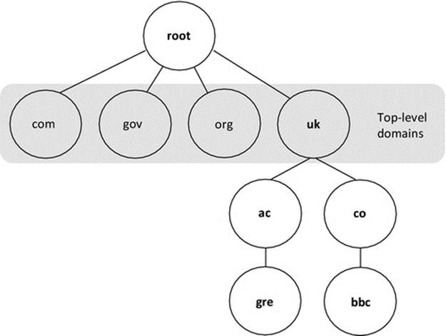
FIGURE 6.15 The inverted tree structure of the domain namespace.
Figure 6.15 shows a tiny fraction of the domain namespace, including the root, four top-level domains, and a couple of lower branches. The leftmost of these two branches shows the gre.ac.uk domain that is a subdomain of the ac.uk domain that in turn is a subdomain of the uk domain. Similarly, the right branch shows the bbc.co.uk domain that is a subdomain of the co.uk domain that in turn is also a subdomain of the uk domain.
There have been several implementations of DNS. Berkeley Internet Name Domain (BIND) is the most popular and thus the most important. BIND is the implementation on which the following discussion is based.
BIND's implementation limits the namespace tree's depth to 127 levels, and each node in the tree has a simple label (name) that can be up to 63 characters in length and must not contain dots. This is a massive namespace and it is difficult to imagine it ever being exhausted. However, as mentioned previously, short names and short paths are more desirable because they are more memorable and usable for humans.
The domain name of a node is the sequence of labels on the path from the node to the root, moving up the tree, with dots separating the names in the path. The root label is often “silent.” For example, in Figure 6.15, the node labeled “gre” has a domain name ofgre.ac.uk while the node labeled “bbc” has bbc.co.uk as its domain name.
If the root domain does appear, the name is written with a trailing dot, i.e, the root is signified by a null final label. For example, gre.ac.uk. could be used to represent the domain name of the gre node in Figure 6.15. Names that are written with this trailing dot notation are termed absolute, as the name is relative to the root and thus unambiguously specifies the node's position in the tree. Absolute domain names are also known as fully qualified domain names (FQDNs).
6.5.2 DNS Implementation
DNS consists of the hierarchical domain-based naming scheme (discussed above) and a database to hold the naming information. The database is distributed due to a number of factors that include the vast size of the namespace and the massive amount of data that must be held to relate the names of resources to their position in the namespace and also to their IP address.
The distribution is performed in a way that mirrors the structure of the namespace itself, so, for example, (referring to Figure 6.15) there would be a part (segment) of the database held at the root level, which contains the details of the top-level domains (i.e., the next level down the tree). The information held in this root segment of the database includes the address details of the database component in each of the top-level domains, so the queries can be directed to them if necessary. It is important to realize that due to the vastness of the namespace, it is not feasible to hold the entire database at the root (or at any other node) as it would take too long to search and thus impact on responsiveness. Instead, if a query to the root node requires information for the domain gre.ac.uk, as an example, then the query will be passed down to the uk top-level domain (because the database segment at that level will contain data relating to the ac.uk domain and the root node does not). The uk domain database segment would be searched to find the address of the ac.uk domain database segment, and the query is then passed down another level (because the ac.uk domain database segment will hold details of the gre.ac.uk domain, and the uk domain database segment does not). The ac.uk domain database segment is used to lookup the address of the database segment within the gre.ac.uk domain and the query is passed down yet again. As the gre.ac.uk domain is a leaf node in the namespace tree, the database segment within the gre.ac.uk domain should contain details of all the resources within the domain such as specific computers, e-mail inboxes, and Web pages.
The example above illustrates the very important way in which the namespace structure is used to achieve name resolution: the actual domain name itself describes how to find the required data, i.e, by working down the tree in the reverse order of the components in the domain name. So for gre.ac.uk, it is possible to start at the root and then visit the uk domain, the ac.uk domain, and finally the gre.ac.uk domain.
However, DNS would be inefficient if every query had to go to up to the root database. Referring once again to Figure 6.15, consider what would happen if a user in the gre.ac.uk domain requested to open a Web page held in the bbc.co.uk domain (such asbbc.co.uk/weather). The query (for bbc.co.uk) is first passed to the user's local DNS component (which is located at gre.ac.uk in this case). The gre.ac.uk database segment does not contain details of the target domain, so the query is passed up a level, to the ac.ukdomain. The ac.uk database segment also does not contain details of the target domain so the query is passed up again, this time to the uk domain. The uk domain database segment does contain details of the co.uk domain, which is the topmost portion of the target path, so the query is this time passed down the tree to the co.uk domain and subsequently to the bbc.co.uk domain. The very important point here is that the query did not travel up to the root level; it was only passed up the tree until a common point in the path was found in which case the target was known to be lower than that point in the tree. This is very significant in terms of understanding the way searches are performed across the distributed database and also in terms of understanding the way in which the tree structure contributes to scalability.
The distribution of the database facilitates scalability of the DNS service (because each segment of the database is restricted in size as it only needs to contain information for the domains connected to it at the next level down the tree and also extensibility of the namespace itself (because the addition of new domains only incurs the registration of the domain at one level above; the new subtree of data relating to the new subtree of namespace will be held in new database segments at the nodes in the new tree itself).
The tree structure by which the distribution is performed facilitates local control of the database segments within specific domains while also allowing the data in each segment to be available across the entire DNS service and allowing for searches to be performed efficiently across multiple database segments.
The localization of control in turn facilitates replication of database segments at the domain level. That is, a particular database segment can be replicated to achieve robustness and enhance performance. The replication factor can differ from one domain to another, to match the name resolution workload of the domain.
DNS has a client-server architecture. A name server is a program that manages a segment of the DNS database. A DNS client (called a Resolver) is an entity requiring the name resolution service of DNS. The name servers make their database segments available to the resolvers through a request-response protocol.
A resolver is usually a library routine used by application developers and is built into end-user applications (such as a Web browser) so that DNS functionality can be accessed automatically when needed from within applications. gethostbyname is a popular DNS resolver for C and C++ (see footnote for Java and C#1), provided as a library routine as part of the Berkeley sockets API.
Figure 6.16 illustrates the use of a DNS resolver called gethostbyname, which is a library routine that can be embedded into applications so that they can directly make DNS requests to resolve the names of computers or other resources into IP addresses. Activity D2 (below) provides an opportunity to explore the behavior of this resolver in action.
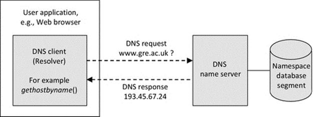
FIGURE 6.16 A resolver (the DNS client side) can be embedded into a user application.
The scenario illustrated in Figure 6.16 works as follows: (1) A user application executes up until a point where it requires a domain name to be resolved. (2) At this point, the gethostbyname routine is called, passing in the required domain name as a parameter. (3) A DNS request is sent to a DNS name server. (4) A DNS response, containing the IP address corresponding to the supplied domain name, is returned.
The behavior is more complex if the local name server cannot resolve the name requested, as depicted in Figure 6.17.
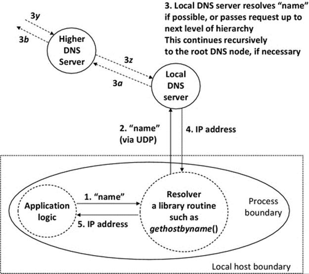
FIGURE 6.17 Hierarchical name resolution in DNS.
Figure 6.17 illustrates the behavior that occurs when the local DNS server is not able to resolve a DNS request. In step 1, the application logic makes a local function call to the gethostbyname resolver. In step 2, a DNS request is issued to the local DNS server instance. If this server could resolve the requested name, it would send back a DNS response directly to the resolver. However, in this case, it is unable to resolve the request so has to pass it up to a DNS server at the next highest level in the tree (this is shown as step 3a in the figure). This passing up procedure is repeated as many times as necessary (see step 3b) until a point is reached where the DNS server can resolve the name. The resolved address is passed back down the levels until it reaches the original DNS server (steps 3y and 3z). The local DNS server then sends a DNS response back to the resolver (step 4). The internal behavior of the DNS system is transparent to the resolver, such that it does not know that the request was passed up to additional DNS servers; the response from the local DNS server to the resolver is the same whether it was resolved locally or not. Finally, the gethostbyname function returns the required IP address details to the application logic (step 5).
6.5.3 DNS Name Servers: Authority and Delegation
Zones: A zone is part of the domain namespace and is associated with a particular named domain. A DNS name server generally has complete information about a particular zone; in which case, the name server is said to be authoritative for that zone. Being authoritative means that it holds the original data for the resources in the zone (i.e., that the information has been configured by the domain administrator or through dynamic DNS methods that support automatic update of records, as opposed to being data that have been supplied through queries to another name server).
Delegation: A zone is a subset of a domain. The difference between a zone and a domain is that a zone contains only the authoritative subset of domain names and not the domain names that are delegated elsewhere (i.e., another name server has authority over that portion of the domain).
Delegation involves assigning responsibility for part of a domain to another organization or assigning authority for subdomains to different name servers. Figures 6.18 and 6.19 illustrate the difference between zones and domains where delegation is present.
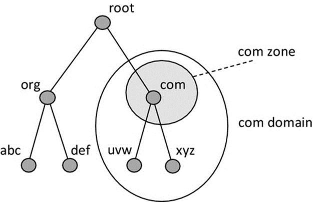
FIGURE 6.18 Delegation example 1: the responsibility for the uvw.com and xyz.com subdomains of the com domain has been delegated to their owner organizations.
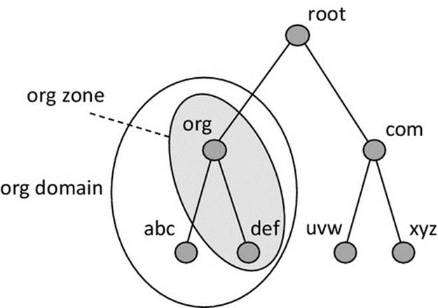
FIGURE 6.19 Delegation example 2: the responsibility for the abc.org subdomain of the org domain has been delegated to the abc owner organization. However, the org domain remains responsible for the def.org domain.
Figures 6.18 and 6.19 show the way in which the zone boundary reflects the limit of authority of the respective name servers. In Figure 6.18, the com name server has delegated responsibility of the subdomains to the organizations that own those domains. This is the most common approach as it prevents the size of the higher-level zone becoming too large, which would increase the workload of its name servers and potentially impact on performance and scalability. In Figure 6.19, the org zone extends to include the def.orgsubdomain; this means that the org name server remains authoritative for the def.org domain.
6.5.4 Replication
DNS name servers (and therefore the domain name data they hold) are replicated for three main reasons:
• Robustness. As mentioned earlier, almost all Internet activity is in some way dependent on DNS to resolve resource names into IP addresses. The distribution of the DNS namespace across multiple domains, each with their own name server, protects against any single failure of a name server affecting the entire system. However, failure of any name server would render the part of the namespace that it was authoritative for unobtainable. Replication is therefore performed at the domain level to provide resilience against failure of any single DNS server.
• Performance. A name server must deal with all requests that require an authoritative answer for its zone. This can become a performance bottleneck, especially in large or very popular zones. Replication shares the lookup burden over two or more name server instances.
• Proximity. The closer a name server to the requestor, the shorter the round-trip network journey and thus the shorter the resolve time. Domains are logical concepts (more obviously near the root of the tree, consider.com that has no geographic basis), and there is no requirement that the replicas of a particular domain's name server are geographically close to each other. .com name servers could be located in the United States and Europe, reducing average round-trip times for service. Leaf domains are more likely to be linked to specific organizations with a physical footprint and thus a link to a specific geographic location. Even so, for international organizations, it may still be beneficial to host multiple replicas of the domain's name servers at different offices around the world.
There two types of name server: primary master servers and secondary servers (also called slave servers). Once running, the secondary server is a replica of the master server, enhancing robustness (through redundancy) and enhancing performance (by sharing the zone's name resolution workload with the master server).
A primary master name server gets its data (for the zones that it's authoritative for) from the host it runs on, i.e., a locally stored file (this is the master copy of the data for the zone). A secondary name server gets its zone data from another server that is authoritative for the zone (such as the primary master or another secondary server). When a secondary server initializes, it contacts an authoritative name server and pulls the zone data over; this is known as a zone transfer. The zone transfer concept can greatly reduce administrative load; the secondary name server may not need any direct administration as it (indirectly) shares the master copy of the zone data.
6.5.5 Name Resolution in More Detail
There are two forms of name resolution query:
• Iterative queries require the name server to give the best answer it already knows. There is no additional querying of other name servers. The best answer might not be the actual address required, but instead, the name server may refer the requester to a closer (in the logical tree) name server that it knows of. Referring back to Figure 6.15 for an example, if the uk zone name server were asked to resolve the name gre.ac.uk, it would refer the requester to the ac.uk zone name server, as this is closer to the target domain and the uk server does not know how to resolve the whole name.
• A recursive query is one where the recipient name server asks other name servers for help in resolving a request (these requests must be iterative queries). The name server originally receiving the recursive query must return the final answer, i.e., the resolved IP address; this is to prevent excessive complexity and latency if recursive queries could be answered with referrals. Any referrals received must be followed, resulting in further iterative queries being sent to other name servers. Recursive queries place most of the burden of resolution on a single name server, as illustrated in Figure 6.20.
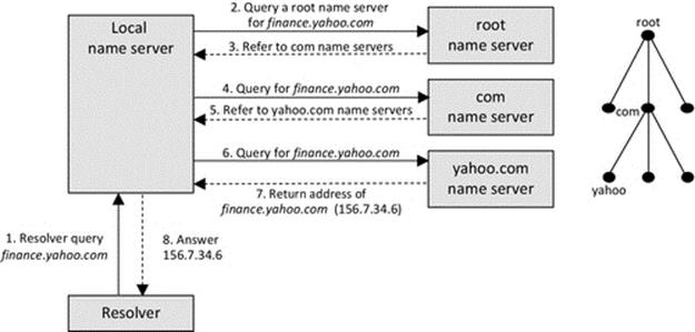
FIGURE 6.20 Resolving a domain name request using a mix of recursive and iterative queries.
Figure 6.20 depicts the usage of the two types of query, in an example to resolve the address of the domain finance.yahoo.com, in 8 steps:
Step 1. A resolver embedded inside an application issues a recursive query to its local name server. This implies that the local name server must return the required address and cannot send back a referral.
Step 2. The local name server does not know any part of the domain name in the request so it issues an iterative query to a root name server.
Step 3. The root name server does not know finance.yahoo.com but it does know com, which is logically closer in the domain name tree than the root, so it refers the requesting local name server to a com name server.
Step 4. The local name server issues an iterative query to a com name server.
Step 5. The com name server does not know finance.yahoo.com but it does know yahoo.com, which is logically closer in the domain name tree than the com, so it refers the requesting local name server to a yahoo.com name server.
Step 6. The local name server issues an iterative query to a yahoo.com name server.
Step 7. The yahoo.com name server knows finance.yahoo.com, because it is within the zone for which the name server is authoritative, so it returns the corresponding IP address to the local name server.
Step 8. The local name server returns the IP address to the resolver (this is the result of the original recursive query).
6.5.6 Caching in DNS
Caching can be implemented at either the client or server side of DNS (or both) to improve performance:
• DNS caching name servers store the results of DNS queries so that if requested again, the answer can be provided immediately from the cache storage, cutting down on the amount of communication occurring between servers and reducing the latency of the request. Caching servers store results for a limited period of time, which is indicated in the domain name record. This means that the cache-holding time is based on the resource itself and thus can be made shorter for more dynamic resources that may be relocated.
• DNS clients can also keep a cache of name-to-address mappings, avoiding the need for repeat queries to name servers for the same resource in a short period of time. This can significantly reduce the load on the local DNS server and enhance responsiveness, since cache access time is much shorter than the time it takes to get a name resolved by contacting a name server.
6.5.7 Exploring Address Resolution
Activity D2 investigates the use of local name resolvers. Specifically, the use of the gethostbyname library method is explored, using the DNS_Resolver example application. The activity is concerned with the way in which the gethostbyname resolver is used to find the IP address of the application's host computer.
Several of the sample applications that accompany the book (in C++, Java, and C#) provide further examples of the use of DNS resolvers such as gethostbyname. Server components make use of a local resolver to find the IP address of their host computer; this address is used to bind a local port so that clients can subsequently make connection requests. In some client components, the local host address is found using a resolver and is used as a default address with which to attempt to connect to the server, as many of the applications can be run for experimental purposes with both client and server on the same computer.
Activity D2
Exploring the gethostbyname DNS Resolver
The gethostbyname library method enables a software engineer to make DNS lookup requests from within applications. In this activity, we shall first run an application to see the use of gethostbyname in action. We then inspect the relevant section of the application's source code to marry up the behavior with the program logic.
This activity is based on the DNS_Resolver application that has been designed specifically to explore the way in which the gethostbyname DNS resolver can be embedded into user applications.
The DNS_Resolver application demonstrates two main uses of gethostbyname: firstly, to enable an application to find its own IP address (the IP address of its host computer) and, secondly, to enable an application to find the IP address of a computer or domain, based on its textual name.
Learning Outcomes
1. To gain an appreciation of the need to embed name resolvers into application programs
2. To gain an introductory understanding of function of the gethostbyname name resolver
3. To gain an appreciation of the way in which gethostbyname is used to find out the local computer's IP address details
4. To gain an appreciation of the way in which gethostbyname can be used to find out the IP address details of a named computer or the IP address associated with a domain name
Method Part A: Appreciating the Need to Embed Name Resolvers into Application Programs
Run the DNS_Resolver application on several different computers. Note that in each case, the application detects and displays the list of IP addresses of the host computer.
Use the built-in name-to-IP address resolver to resolve the names of other computers in your local network or try external domain names.
Expected Outcome for Part A
You should see the correct IP address(es) displayed. Your home computer will typically only have one IP address. However, many computers have several IP addresses depending on their configuration and use. A computer may, for example, be configured to work with two different networks, one wired and one wireless, in which case it will have two IP addresses.
The screenshot below shows the program running on a computer with the computer name RICH_MAIN and IP address 192.168.100.2. You can also see that the IP address resolver has been used to find the IP address associated with the domain namebbc.co.uk.

Method Part B: Using gethostbyname to Find the IP Address of the Local Host (Computer)
Look at the source file named DNS_ResolverDlg.cpp. Study the code and locate the part where the local hosts' IP address is obtained.
Expected Outcome for Part B
The relevant code is contained within the method GetLocalHostAddress_List(). Here is the code:
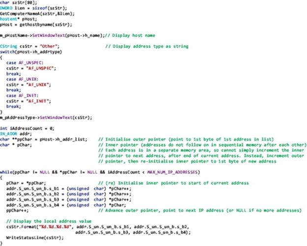
This code works as follows:
First, the computer's textual name is found. A character array is declared as a buffer, of size 80 bytes, to hold the computer's host name. The variable lLen is initialized with the size of the buffer. The GetComputerNameA() method is called, which places the computer's textual name in the character array (the lLen parameter prevents overrun of the buffer if a very long computer name has been used).
Second, the computer's IP address is found by passing the computer's name as a parameter to the gethostbyname method. The result of the gethostbyname() call is a special hostent structure that contains the computer's name, address-type code, and a list of IP addresses (if there are more than one).
Next, the computer's host name and address type are displayed.
Finally, the while loop iterates over the address list (which is part of the hostent structure) and each of the local computer's IP addresses is displayed.
Method Part C: Using gethostbyname to Find the IP Address of a Computer or Domain
Look again at the source file named DNS_ResolverDlg.cpp. Find the section of code where a computer's IP address is obtained based on its textual name.
Expected Outcome for Part C
This functionality is achieved by the event-handler method OnBnClickedResolveButton(). The key part of the code is shown below:

The main difference here is that the name of the computer is provided by the user and not implicitly as in part B of the activity. The computer name is retrieved from the user-interface control and then passed as a parameter to gethostbyname(). The rest of the code works in a similar way to that of part B except that in this case, only the first IP address in the list of addresses is displayed and also that error handling is needed because the user may enter nonexistent computer names or the names of other resources to which IP addresses are not mapped.
Reflection
The DNS resolver gethostbyname enables you to leverage the power of the DNS service within your application. This is a very important concept for distributed applications. If you look at the sample applications provided as support resources for the book, you will find that many of them use gethostbyname.
6.5.8 Reverse DNS Lookup
There are occasions when it is necessary to map a known IP address to an unknown domain name. For example, with eCommerce and online services, it is often desirable to validate that the source of a message is actually where it claims to come from. The ability to trace a source IP address back to a domain name can also be very useful for systems administration and maintenance purposes and is an important part of a computer-forensics tool kit.
Reverse DNS lookup is supported through the provision of two special domains named in-addr.arpa for IPv4 addresses and ip6.arpa for IPv6 addresses. All possible values of Internet address are mapped appropriately in one of these domains.
For explanation purposes, IPv4 will be considered. At the level below in-addr.arpa (level three), there are 256 domains labeled 0 to 255 (i.e., 0.in-addr.arpa to 255.in-addr.arpa). At level four, there are 256 domains for each level three domain (0.0.in-addr.arpa to 255.0.in-addr.arpa up to 255.555.in-addr.arpa). At level five, there are 256 domains for each level four domain. At level six, there are 256 domains for each level five domain. This allows every combination of IPv4 address in the range 0.0.0.0 to 255.255.255.255 to be represented in a corresponding entry in the range 0.0.0.0.in-addr.arpa to 255.255.255.255.in-addr.arpa.
Therefore, each possible Internet address maps directly onto a level six domain in the in-addr.arpa domain space. The Internet address is written backward so that the most significant byte of the address is closest to the root of the tree. For example, IP address 212.58.244.20 is represented in the in-addr.arpa domain space as 20.244.58.212.in-addr.arpa. When a query for a domain in the in-addr.arpa domain space is received by a name server, data describing the domain to which the supplied IP address relates are returned.
Here is a simple reverse DNS lookup experiment to try: Step 1, use the DNS_Resolver application (see activity D2) to resolve a domain name that you are familiar with (e.g., the domain name bbc.co.uk was resolved to IPv4 address 212.58.244.20). Step 2, identify one of the freely available online reverse DNS lookup tools and request a reverse lookup for the domain name constructed in the form reversed-IPv4-address.in-addr.arpa (for the bbc.co.uk example, this is 20.244.58.212.in-addr.arpa). The result should be the original domain name you started with (for the bbc.co.uk example, the query returned fmt-vip71.telhc.bbc.co.uk, which is indeed within the bbc.co.uk domain).
6.6 Time Services
A general requirement for many distributed applications is that processes each have access to an accurate local clock or can otherwise get an accurate time value when necessary (e.g., through a time service). The following section describes time services such as NTP; these provide a time value that can be used however needed by applications (this could include setting the physical clock at the local computer). Subsequent sections deal with physical and logical clock synchronization, respectively, and also discuss the various ways in which time values are used in distributed applications.
6.6.1 Time Services
The Internet Time Service (ITS) is a collection of time service protocols provided by the National Institute of Standards and Technology (NIST). The NIST services are hosted on a moderate number of computers around the world, primarily in the United States, owned by commercial organizations and universities. The replication of the service over numerous geographically distributed sites ensures that the service is robust, and because the time service load is shared across the servers, it is responsive.
NIST currently supports the DAYTIME protocol, the TIME protocol, the Network Time Protocol (NTP), and the Simple Network Time Protocol (SNTP), a simplified version of NTP. Of these, the popularity of the first two is in decline as they are less accurate and less efficient with respect to communication resources than NTP. At the time of writing, NIST is encouraging users of those protocols to migrate to NTP.
Externally, the NIST servers offer the time services mentioned above. Lists of NIST time servers are available on the Internet, and users either can request time services directly from a geographically local server or can use the global address time.nist.gov, which is resolved to different physical time server addresses in sequence to share out the load on the time servers. Using this address also has the advantage of reliability as it will always be resolved to a currently working server, whereas contacting a specific server by its address runs the risk that the server is unavailable.
6.6.1.1 TIME Protocol
The TIME protocol is currently supported by NIST time servers but has several weaknesses when compared with NTP and thus is included here briefly for comparison purposes only.
This protocol provides a 32-bit value that represents the time in seconds since January 1, 1900. Due to the 32-bit resolution, the format can represent dates in an approximately 136-year range; i.e., it will be redundant by design in 2037. The simple data format does not allow the transmission of additional information such as daylight saving time or information about the health status of the server.
6.6.1.2 DAYTIME Protocol
This protocol provides significantly more information than the TIME protocol. Designed in 1983, it is inferior to NTP. Brief details are included here for comparison purposes.
The time is sent using standard ASCII characters with a simple code format. In addition to the actual time and date information, it also includes a code to signal daylight saving time and an advance warning code that a leap second is to be added at the end of the current month. There is also a code to signal the health of the server, which is important for time-critical applications to be able to have confidence in the accuracy of the time service values.
The DAYTIME protocol adds a fixed offset (currently 50 milliseconds) to the advertised time value to partially compensate for network transmission delay.
6.6.1.3 Network Time Protocol (NTP)
In use since 1985, the NTP is the most popular Internet time protocol. It is based on UDP, therefore having low networking overheads and low service response latency because it does not need to establish a TCP connection.
An NTP client periodically requests updates from at least one server. When multiple servers are used, the client averages the received time values, ignoring any outlier values (in a similar way to that used by the master server in the Berkeley algorithm; see later text).
NTP provides greater precision than the TIME and DAYTIME protocols. It uses a 64-bit time stamp value representing the time in seconds since January 1, 1900, and has a resolution of 200 picoseconds (although this level of precision cannot generally be leveraged due to dynamic network delays that can fluctuate by values significantly larger than this).
The use of NTP within distributed applications has been discussed in Chapter 3, where it is also used as an example of a request-reply protocol and explored in a practical activity using an NTP client application that has been built into the Distributed Systems Workbench.
An alternative to the continual operation of NTP is the similar but more lightweight SNTP that supports single time requests when needed (as opposed to the periodic nature of NTP usage).
Figure 6.21 illustrates infrastructural features of the NIST time service provision, showing the differentiation between the internal and external aspects of the service. The internal service configuration synchronizes the NIST internal time value to UTC/GMT and also synchronizes the NIST time servers to each other. Externally, NIST provides a number of time services that each serves the same time value but in different formats and with different levels of precision. Of these services, NTP and SNTP are the most important due to communication efficiency and precision of time values.
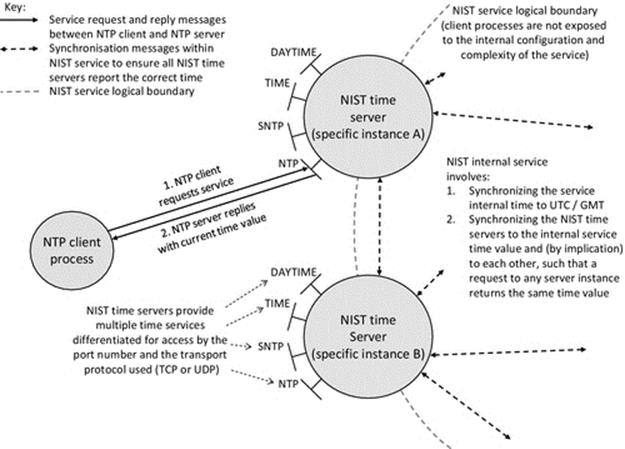
FIGURE 6.21 Infrastructural aspects of the NIST time service provision.
All of the NIST time services provide transparency to clients in the sense that clients do not need to be aware of the internal configuration and behavior of the NIST system, of the multiplicity of time services, or of the replication of NIST time servers.
6.6.2 Physical Clock Synchronization
Each computer has an electronic clock that keeps track of wall-clock time (time in the real world, as shown by a clock). These electronic clocks (called physical clocks) tend to be accurate to within a few seconds each day, but can drift over longer periods, such that the clocks on different computers in the same system show significantly different times. Physical clock drift can be problematic for any applications whose behaviors are time-dependent or need to record the time at which events occur.
Factors that affect the rate of clock drift include the quality of the electronics that constitutes the clock circuit and the ambient temperature of the clock's environment (which can fluctuate significantly if the clock is contained within the casing of a computer with a heat-generating CPU and cooling fans running). Therefore, even with the best-quality clock circuitry, it is not possible to precisely predict drift and thus compensate for it by software techniques.
A wide variety of types of distributed applications require that the clocks at each processing node within a distributed system must be synchronized to ensure consistency and accuracy. Clocks are used for various purposes:
• To define an ordering of events (e.g., when constructing models of real-world systems based on sensed data collected from many sites, such as weather prediction).
• To coordinate events to occur at the same wall-clock time (e.g., to start processes simultaneously or with a specific time offset, in a controlled physical environment such as an automated production facility).
• To record the passing of wall-clock time (e.g., measuring the interval between events in systems, such as network message arrival, and another example is transport display systems where the expected time of arrival (of busses, trains, or aircraft) has to be computed and displayed alongside current time or displayed as an offset from current time).
• As a measure of performance (this is achieved by comparing the beginning and end times of a particular activity; this could be a system activity such as measuring how long the system takes to perform a particular task or a real-world activity such as measuring the acceleration of a vehicle based on multiple samples from speed sensors or a reaction timer as part of a game).
• Time values as a signature, or identity (e.g., for indicating the creation and modification times of resources such as files and a second example is the within-security schemes, where message time stamps are used to prevent message replay).
• To permit reasoning about the global state of the system based only on local information (e.g., within heartbeat-based systems to determine if another process is present, such as within election algorithms (see earlier section) in which heartbeats are awaited only for a limited time window).
• To provide globally unique values (a precise time stamp is a component in a globally unique identifier (GUID). The GUID also contains a location-based component (IP or MAC address) and a large random component. This combination of values yields a number that cannot occur again. This is because if generated on the same computer, the new GUID will have a different time component (or even if performed in rapid succession such that the time stamp does not change, the random component will) and if generated on two computers at the same time, it will have different location components). GUIDs are thus vital in systems such as distributed databases and distributed object-based applications where resource identifiers must be guaranteed unique system-wide yet need to be locally generated without having a central ID issuing service).
In some distributed applications, the wall-clock time accuracy is of prime importance, while in others, the actual precision by which the clocks are synchronized is more important than the wall-clock time accuracy.
The crux of the challenge for synchronizing physical clocks in loosely coupled distributed systems (i.e., those that consist of independent computers that communicate over computer networks) is that any message sent across the network encounters delay, and the delay has some fixed and some variable components. An example of a fixed delay component is the propagation delay that is directly related to the distance the signal has to travel through cables, and an example of variable delay is the queuing time that a message spends in routers, which is traffic-dependent. The variable components of the message delay mean that it is not possible to precisely know the arrival time of any message sent between two computers even if its transmission time is known precisely.
The fact that message delays cannot be precisely known means that it is not possible to transmit a time value between two computers while preserving its wall-clock meaning, so as to accurately set the clock at the recipient computer. For example, consider that at exactly 12 noon, a time stamp is sent from computer A (whose clock accurately reflects wall-clock time) to computer B, across a computer network. When the time stamp arrives, its value will still be 12 noon but its meaning is now no longer accurate because the actual time is a little bit past 12 noon; but the recipient does not know how much time has elapsed while the message was in transit, so they cannot make the adjustment required. If the time stamp is used literally, then some error creeps in. For systems connected over physically short distances with few intermediate routers, this error value may be on average much less than one second and the resulting small time difference between clocks may be acceptable for some systems.
There are various ways to improve on this basic starting position of simply sending the wall-clock time and using the resulting value literally. However, since network delay is nonconstant, whatever technique is performed, the outcome is described as a loose synchrony.
6.6.2.1 Physical Clock Synchronization Techniques
A time service must synchronize the clock of the local computer with that of other computers in a network. One approach is to designate some time servers as “reference” servers that provide an accurate, stable time source to clients on the network. In order to do this, the reference servers must synchronize their own host's physical clocks to agree with some real-world clock aligned with UTC/GMT (see the discussion on NIST time services above). Clients and nonreference time servers adjust their clocks to agree with the time reported by a reference server.
The problems involved in this synchronization process are that clocks can drift, which can lead to differences between local clock times, network delays are unpredictable (these points are explained above), and also processing delays (due to the presence of other processes) at both the sending and receiving computers of a network message further introduce a variable delay in reading a clock value or writing a clock value, respectively.
6.6.2.2 Cristian's Algorithm
This technique uses a time server that is synchronized to Coordinated Universal Time (UTC). The clocks of other computers in the local network are set by querying the server. The distinguishing feature of Cristian's technique is the way it takes account of network latency. The round-trip delay (d) is measured. The assumed one-way latency (d/2) is added to the time value when sent to a requesting computer, to improve the accuracy of the value upon arrival (d/2 time later) (see Figure 6.22).
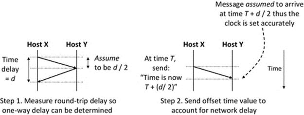
FIGURE 6.22 Cristian's algorithm for physical clock synchronization.
Figure 6.22 shows the principle of estimating network delay used in Cristian's algorithm. The concept is simple: measure the round-trip time for a message to be sent to another computer and a reply to be sent back; this takes into account the delay in each direction in the network and also the processing delay at the two computers themselves when dealing with sending and receiving the messages. This approach uses the same clock to measure the start time and end time of the round trip; this is the clock of host X in the figure, hence avoiding any inaccuracies arising from the fact that the clocks are not yet synchronized. Therefore, the assumption is that if the total delay is halved, then this is representative of the delay in one direction. This halved value can thus be added as an offset when sending the time stamp so that when it arrives, having suffered the equivalent delay, it is realigned with wall-clock time, and thus, the recipient can set its clock accurately. However, while being generally sound and an improvement over not adjusting for network delay, there are still three sources of error with this technique that can affect the accuracy of the d/2 delay assumption: (1) Network delays are time-varying; (2) network delays can be different in each direction, even on the same link; and (3) the processing delay on each computer is also time-varying.
6.6.2.3 The Berkeley Algorithm
The Berkeley algorithm aims to synchronize all clocks in a group of time servers. The first step is to elect a master, which coordinates the synchronization activity (see the earlier section “Election algorithms”). The master polls the other time servers, who respond by sending their current time values back to the master. During this step, the master also determines the round-trip time between itself and each of the respondents, in the same way that Cristian's algorithm does it.
Based on all of the received values and its own clock value, the master computes the average time (significant outlier values are ignored to prevent distortion of the result). There is an assumption that errors cancel out to a certain extent; however, if all clocks are fast or all are slow, the resulting average will also be fast or slow, respectively.
The master calculates the amount by which each individual time server process must adjust its clock. This takes into account the current time difference (between the specific server's current clock and the computed average time value) and also adds an adjustment equivalent to half of the round-trip delay measured for the specific time server. The resulting clock offset values are then sent to each time server process, and the master updates its own clock locally. Upon arrival of these offsets, the recipient computer knows how much to adjust its clock to bring it to the same value as the group average (because the network delay has already been compensated for). The Berkeley algorithm is illustrated in Figure 6.23.
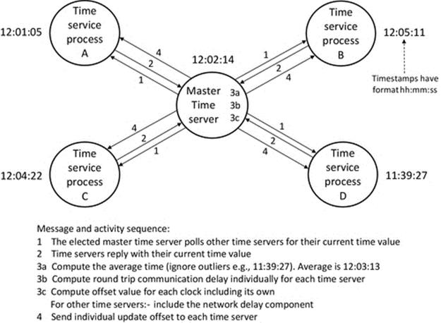
FIGURE 6.23 The Berkeley clock synchronization algorithm.
Figure 6.23 shows the operation of the Berkeley algorithm, contextualized with an example. The scenario assumes that the master has already been elected (this is realistic as the election of a master should be a rare event occurring only when a previous master has crashed). The Berkeley algorithm operates periodically. The figure shows one of these periodic clock update episodes.
In step 1, the master polls all time servers in the group for their current time values; they respond in step 2. The master then computes the average time of all clocks including its own but excluding any that is significantly different from the average value, to avoid distortion by unreliable clocks (step 3a). In step 3b, the master estimates the network delay to each specific time server (using the half round-trip delay technique as used in Cristian's method). The master then combines the results of step 3a and 3b to provide a unique clock offset value for each time server (step 3c) and sends these values to the time servers in step 4.
There are two update scenarios that occur at time servers when applying the received offset value:
• When the clock adjustment is forward (e.g., time server A in Figure 6.23 moving its clock value from 12:01:05 to 12:03:13), the adjustment can be applied immediately. This is because the clock has never showed the time values that are being skipped, and thus, no events could have occurred and been time-stamped with those values. Therefore, moving the time forward cannot confuse the representation of the ordering of events that have already happened.
• When the required clock adjustment is backward (e.g., time server B in Figure 6.23 moving its clock value from 12:05:11 to 12:03:13), the situation is more complex. Actually, moving clocks backward is undesirable in systems where events are time-stamped and where the history of event ordering is important. The problem is that the clock has already held time values in the range of times that will be repeated, and by setting the clock back could lead to inconsistency in the event order history.
For example, consider a scenario in which an event E1 has already occurred at time 12:04:17 on a computer that gets its time updates directly from time server B (in Figure 6.23). When the time gets to 12:05:11 (as perceived by that specific time server), the server receives a time update from the master, requiring it to set its clock back to a time earlier than the stored time stamp of E1. Shortly afterward, some of the computers that get their time updates from server B have updated their local clocks. An event E2 then occurs at one of those computers, at the time 12:03:55. Now, the system is inconsistent because event E1 actually happened before event E2, but their time stamps indicate that E2 happened first. An example of how this inconsistency could materialize into a real problem is a distributed file system in which there are multiple versions of the same file. Let events E1 and E2 represent the last modification events of two versions of the same file, and thus, the most recent time stamp implies the latest version of the file. A particular application may inspect the time stamps and wrongly assume that the file version with the E1 time stamp is the most up-to-date copy of the file.
Rather than adjusting the clock backward, there are two better alternatives: (1) Halt the clock from updating, for a period equivalent to the offset sent from the master, so that wall-clock time catches up with the time shown by the clock, and (2) slow down the physical clock's tick rate (which is described as clock slew), so that the correction is applied over a longer period of time rather than instantly. Both of these solutions avoid the inconsistency that can arise when previously shown clock values reoccur.
6.6.3 Logical Clocks and Synchronization
Event ordering can be achieved without the use of real-time clocks. If real-world time values are not required, then a simple mechanism can be devised for event ordering. The only requirement in such a case is the need to know the sequence with which the events occur.
A logical clock is a monotonically increasing integer value. In other words, it is a number that increases by one increment each time an event occurs. Logical clocks do not capture the passing of wall-clock time; instead, they are used to indicate the relative time at which events occur. The “time” values are a simple sequence of numbers.
Consider a set of three events that occur at different times, as shown in Table 6.2.
Table 6.2
Wall-clock Event Times
|
Event |
Wall-clock time |
|
A |
02:05:17 |
|
B |
02:05:19 |
|
C |
07:49:01 |
By looking at the wall-clock times of the events shown in Table 6.2, we can see that the events occur in the sequence A first, then B, and finally C. We can convert this to a logical clock numbering, as shown in Table 6.3.
Table 6.3
Logical Clock Event Values
|
Event |
Logical clock value |
|
A |
1 |
|
B |
2 |
|
C |
3 |
As illustrated in Table 6.3, the logical clock increases monotonically each time a new event occurs. Notice that the logical clock representation is purely concerned with sequence; it shows that event A happened before event B and that event B happened before event C. In Table 6.2, where a wall-clock sequencing is used, it is possible to see the relative timing of the actual events (event B follows soon after event A, and then, there is a relatively long interval before event C). The time element is discarded when using a logical clock representation.
6.6.3.1 Event Ordering Using Logical Clocks
When two events a and b occur in the same process and a occurs before b, then event a is said to have happened before event b.
Message sending is split into two events: when a message is sent from one process to another, the “message sent” event happened before the “message received” event. This is a fundamental requirement to represent the fact that all messages have some transmission delay, and this is a very important concept when considering the correctness of distributed algorithms. In a distributed system, it is possible for two processes to each send a message to the other process and for both send events to have occurred before either of the receive events. This is just one of the possible orderings that could occur; another could be that one process sends a message to the other process that receives that message before sending a reply message back.
When two events are related together in some application-meaningful way (e.g., in a banking application, they could both be transactions on the same bank account), then they are said to be causally related. However, using the same banking example, events that update different bank accounts are not causally related; their relative ordering has no consequence to the banking application itself.
For a pair of causally related events a and b, if event a happened before event b, then we express this using the “happened before” relation written as a → b. This is also described as causal ordering. New causal orderings can be built up from existing causal ordering knowledge. For example, a simple but very important rule is:
![]()
This states that if event a occurs before b and b occurs before c, then a occurs before c.
Groups of causally related events can overlap other groups of causally related events, but each group of events is not causally related to the events in the other groups. In such cases, the global ordering of the entire system must respect the causal ordering sequences that exist. To clarify, consider, for example, sequences of ATM cash withdrawals for two unrelated customers a and b. Each customer makes two cash withdrawals on the same day. The events generated are labeled a1 and a2 (for customer a) and b1 and b2 (for customer b).
If a1 → a2 and b1 → b2, then a1 and a2 are causally ordered, and b1 and b2 are causally ordered, but a1 and b1, for example, are not. In such a scenario, the following actual event orderings are possible because they respect the causal orderings:
![]()
However, {a1 b2 a2 b1} is not possible because it violates the b1 → b2 relationship. Similarly, {b1 a2 a1 b2} is not possible because it violates the a1 → a2 relationship.
6.6.3.2 Logical Clock Implementation
Ordering of events at a process can be achieved by defining a logical clock mechanism. Each process maintains a local variable LC called its logical clock that relates each event occurrence to a unique integer value. Before the initial event, all processes must set their logical clocks to zero. For consistency across the system, logical clocks must always increase in value as events occur.
An event occurrence causes the logical clock to be updated. Newly created events (e.g., sending a message) are assigned the resulting updated value of the logical clock (this value can be considered the time stamp of the message). For example, if the logical clock has an initial value 4, when a message is sent, the clock will increment to 5 and the message will be sent with a time stamp of 5.
When a message is received, the receiving process updates its logical clock to be greater than the maximum of its current logical clock value and the time stamp of the incoming message, as illustrated in Figure 6.24. The effect of this is to (loosely) synchronize the local logical clock of the process that received the message with that of the remote process that sent the message.
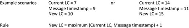
FIGURE 6.24 Logical clock update scenarios on receipt of a message from another process.
Figure 6.24 shows the rule that is applied when a message arrives from another process causing the local logical clock value to be updated and provides two example scenarios. In the scenario on the left, the message arrives with a time stamp value of 9 and is higher than the logical clock value of 7. The new logical clock value is thus 9 + 1 = 10. In the scenario on the right, the message arrives with a time stamp value of 11 but the logical clock value is already higher, at 14. The new logical clock value is thus 14 + 1 = 15.
The progression of logical clock values in a system of three communicating processes is illustrated in Figure 6.25. Notice that for each process, the logical clock values are always increasing according to the “happened before” relationship between events, and the clock update rule is illustrated in Figure 6.24.
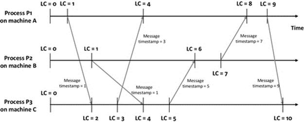
FIGURE 6.25 Logical clock-based event ordering across a distributed system.
Figure 6.25 shows how the logical clock values progress in a scenario involving three communicating processes. The logical clocks are maintained locally by each process, and therefore, they are not tightly synchronized. Instead, a loose synchronization is achieved in which processes only get a hint as to the value of the clocks at other processes when they receive a message from those processes (the time stamp of the message indicating the sender's logical clock at the point when the message was sent). Logical clock values remain static between event occurrences, as the passing of wall-clock time is of no concern.
6.7 Election Algorithms
There are many scenarios in distributed systems where it is necessary to automatically select one process from a group, so that it can perform some specific role. An election algorithm provides the means to do this.
Scenarios where election algorithms are employed include
• replicated services in which coordination is necessary,
• reliable services in which continuation of service despite failures is important,
• self-organizing services in which processes may need to know their status relative to others,
• group communication mechanisms (see later text) in which there is a need to establish a group coordinator.
Election algorithms are therefore a fundamental requirement for many distributed applications. As an example, a replicated database system may require that a single coordinator is maintained, to ensure that updates are propagated to all copies of the database. In such an application, there must always be exactly one coordinator, despite variations in the number of database server instances (e.g., additional servers might be automatically started when the system load increases) and node failures. If there are no coordinators, or multiple coordinators, then the database could become inconsistent. Therefore, if the system enters an illegal state, e.g., no coordinator or multiple coordinators, it must be returned to a legal state as quickly as possible.
6.7.1 Operation Overview
Most election algorithms have a two-state operation, in which instances assume the slave state by default. From this starting point, a single instance is elected to be the master (sometimes called coordinator, or leader). Once elected, the role of the master is to coordinate a particular distributed or replicated service or application. The role of the slaves is to monitor the presence of the master, and upon detection of its failure, they must elect a single new master from the pool of slaves.
Figure 6.26 shows an election occurring after the original master has failed. There are two critical stages to this: firstly, the means by which the remaining processes detect that the master has failed (any delay here impacts on the overall time required to establish a new master) and, secondly, critical stage, the means by which the election takes place (i.e., the negotiation as shown in part c of the figure). It is important that the negotiation is not too communication-intense because that would impact on scalability, as well as wasting valuable network bandwidth resource.
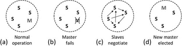
FIGURE 6.26 General operation of election algorithm, showing an election taking place.
Each of the processes involved in the election algorithm runs the algorithm locally. There cannot be a central controller; that would be self-defeating because the central controller could fail, so how would that be replaced? The whole point of the election algorithm is to elect a leader in a distributed way. There are some implications of this: Any of the processes present should be able to become the leader, and even if there is only a single process, there should still be a single leader (the single process must elect itself in such a case).
Figure 6.27 shows a simplified state transition diagram for a generic election algorithm (it does not show the slave negotiation aspect of the behavior). Each participatory process must operate this algorithm and keep track of its own individual state. The diagram shows the only states and transitions between those states that are allowed to occur. This is a very useful way to represent algorithms because it is easy to translate the diagram into program logic. Even though this is a somewhat simplified representation of a generalized algorithm, it illustrates how you can almost read off the program logic from the transition descriptions. Figure 6.28 presents a simplified pseudocode that can be elicited from this particular state transition diagram.
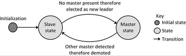
FIGURE 6.27 Generic state transition diagram for 2-state election algorithm.
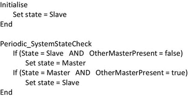
FIGURE 6.28 Simplified pseudocode elicited from the state transition diagram in Figure 6.27.
Election algorithms are distributed algorithms that operate within distributed applications. They have a number of specific design requirements arising from both their distributed nature and the key behavioral requirement that they ensure a single master is maintained.
The nonfunctional requirements are generally the same for all election algorithms and include the following:
• Scalability. The algorithm should operate correctly regardless of how many processes are involved.
• Robustness. This is implied by the very nature of an election algorithm, i.e., to recover from the failure of the master process.
• Efficiency. There should not be excessive communication, particularly in the negotiation phase.
• Responsiveness. There should be low latency in detecting the absence of a master process and subsequently initiating an election.
See also the more detailed discussion of nonfunctional requirements in Chapter 5.
The various election algorithms differ in their design and thus in their internal function. This means the functional requirements can differ from one algorithm to another but generally include the following:
• The proportion of time that a master exists should be very high.
• A replacement must be found quickly if the current master is removed.
• Multimaster scenarios must be detected and resolved quickly.
• Spurious elections caused by falsely detecting master failure should be avoided.
• Normal-mode communication intensity (the number of messages sent under master-present conditions) must be low.
• Election-mode communication intensity (the number of messages and the number of rounds of messages required to elect a new master) must be low.
• Communications overhead (the mean total communication bandwidth required by the election algorithm) must be low.
6.7.2 The Bully Election Algorithm
A number of different election algorithms have been designed. The bully election algorithm is probably the best-known election algorithm. It works as follows:
• Each node is preallocated a unique numeric identifier.
• During an election, the highest ID node available will be elected as master.
• When the master fails, the nodes communicate, in rounds, to elect a new master.
• The nodes enter the election state when they are a candidate for the master role.
• The nodes are eliminated if they receive an election message from a higher-ID node.
By negotiation, they must
• determine which node has the highest ID,
• reach consensus (all nodes must agree).
Figure 6.29 shows the operation of the bully election algorithm. Part a shows the normal single-master scenario. In part b, the master fails, leaving a system of zero or more slave nodes (in this example, there are 4). In part c, the first slave node (1) to notice the absence of the master (by the absence of its heartbeat signals) initiates an election by sending a special message (which also serves to inform all other slaves of its unique ID). In part d, slave 4 joins the election, sending its special election message that causes slaves 1 and 2 to be eliminated (because ID 4 is higher than ID 1 and ID 2). In part e, slave 5 joins the election, eliminating slave 4. If slave 5 does not hear any further election messages in a given short time frame, it assumes that it has won the election (as a result of it having the highest ID) and it elevates itself to master status (part f).
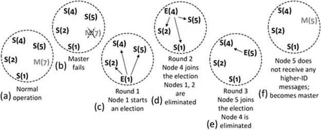
FIGURE 6.29 Operation of the bully leader election algorithm.
Notice that the number of rounds needed to complete an election is dependent on the sequence by which the slaves join the election. The election would be over very quickly if the highest ID slave happens to be the one that first notices the failure of the master, as it would eliminate all other slaves in a single round. In the worst case, the slaves join the election in ascending order, requiring one round per slave (i.e., N − 1 rounds, where N is the size of the original system before the master failed).
6.7.3 The Ring Election Algorithm
The ring election algorithm is similar to the bully election algorithm, but the nodes are arranged in logical ring, and the nodes only communicate with their logical neighbors.
When the master is lost, its neighbors (in the ring) will notice (due to a lack of periodic heartbeat messages). The negotiation phase is achieved by the nodes passing messages around the ring (in several rounds) to establish which is the highest numbered node and to ensure consensus.
Figure 6.30 shows the operation of the ring election algorithm. Part a shows the normal single-master scenario; the nodes are connected in a logical ring that is maintained by periodically sending messages from node to node. The message informs the recipient of the identity of its upstream neighbor and that the neighbor is alive. In part b, the master fails, which breaks the ring. In part c, node 1 notices the absence of the master (by the absence of the expected messages) and initiates an election by sending a special message to its logical neighbor (node 2). In part d, the election message propagates around the ring until the highest numbered remaining node has been identified and all nodes are aware of its identity. In part e, slave 5 elevates itself to master status.
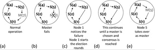
FIGURE 6.30 Operation of the ring election algorithm.
6.7.4 Leader Preelection
Leader preelection is a technique where a backup master is selected while the system is operating normally. If the master fails, the backup detects the failure and takes over as master.
Selection of the backup is still performed by an election algorithm, but the election is done during normal operation (i.e., in advance of the master failing) so the system is leaderless for a shorter time.
Note that the backup can fail before an election occurs; therefore, there is the possibility of wasteful elections to select backup master nodes that are survived by the current master.
As illustrated in Figure 6.31, the purpose of the leader preelection is to preselect a backup leader in advance of any problem with the master, such that under normal operation, both the master and the backup master exist (as in part a of the figure) and both send heartbeat messages to inhibit slaves electing further nodes. When the master node fails (part b), the backup is rapidly able to take over leadership of the service (part c). The latency is only the time needed to detect that the master has failed, the main component of which is the time waiting for the next heartbeat from the master (which never arrives). There is no requirement for additional message transmission or the negotiation associated with elections. As soon as the backup node has elevated itself to master status, it can initiate an election of a replacement backup node (part d). Thus, the amount of time the system is leaderless is very small (the one tuning parameter being the interval between heartbeat messages).
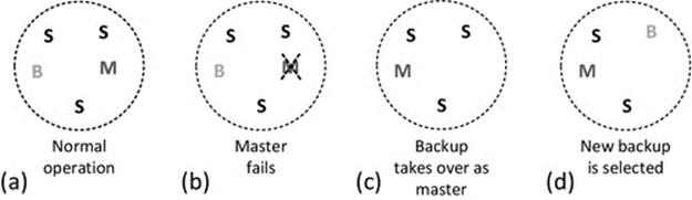
FIGURE 6.31 The leader preelection technique.
6.7.5 Exploration with an Election Algorithm
Activity D3 explores the behavior of election algorithms. It uses a specific election algorithm, the “Emergent Election Algorithm,” which is built into the Distributed Systems Workbench.
The Emergent Election Algorithm is a two-stage algorithm for electing leaders in large systems. It has been designed specifically to be highly scalable and efficient. It achieves this by introducing two additional states not usually found in traditional algorithms:
The idle state is used to separate out a majority of processes (on average, it is all except four processes) that only listen to messages sent by the master and slaves. Processes in the idle state never send any messages.
The candidate state is a transient state that is only used during elections. A process that determines it is a candidate for being the master moves into the candidate state from slave state, prior to becoming master. The process must remain in the candidate state long enough to ensure that there are no other processes still involved in the election. This is used to enforce the rule that there must only be a single-master process present at any time.
The four states of the Emergent Election algorithm are described in Table 6.4. As mentioned above, the algorithm operates in two stages, as this enables a design that is simultaneously highly scalable and also very efficient in terms of the number of messages sent (which is near constant regardless of the system size).
Table 6.4
The Four States of the Emergent Election Algorithm
|
State |
State persistence |
Description of behavior when in the state |
|
Master |
Stable state |
Coordinate the host service |
|
Candidate |
Transient state |
Election participant. After negotiation based on IP address, exactly one candidate node will elevate to master status |
|
Slave |
Stable state |
Monitor the presence of master. Contender for master status (via candidate state) if the current master fails |
|
Idle |
Stable state |
Monitor slave population. Contender to become slave if the pool of slaves is diminished beyond some threshold |
The first stage employs the idle state. This stage separates the majority of processes away from a small active pool of slaves. The idle processes (the majority) never transmit messages; they simply monitor the size of the slave pool. Each slave state process sends periodic slave-heartbeat messages, so by listening for these and counting them over a specific time period, an idle-state process can determine the number of slaves present (i.e., the size of the slave pool). If an idle process' local perception of the slave pool size falls below a lower threshold, the process will elevate to slave state.
Slave-state processes also listen to the slave-heartbeat messages to determine the slave pool size. If a slave process' local perception of the slave pool size rises above an upper threshold, it will demote to idle state. Both the idle and slave state listening periods contain random components to ensure that each process has a slightly different perception of the state of the system, thus ensuring stability (because the processes don't all suddenly switch to either the slave or the idle state, instead a gradual and self-regulating effect is achieved).
The candidate state is used in the second stage of the algorithm to ensure that elections are deterministic, i.e., that only one process elevates to master status, regardless of how many slaves are in the slave pool. The candidate state also plays an important role in preventing false elections, for example, if a master's heartbeat message is lost in the network. This is because a process must remain in the candidate state for a time long enough for several master heartbeat messages to occur, so that even if several were lost, there is a high probability that the candidate will eventually detect a master heartbeat if the master is present.
Figure 6.32 shows how the two stages of this particular algorithm are coupled together by the slave pool, as an idle process must move through the slave state to become master, and vice versa. The composition of the slave pool and thus its size also are emergent properties arising from all of the local interactions between slave and idle processes, whereby the behavior of each is determined by the number of slave messages received in a short time interval. Hence, the algorithm is described as “emergent.”
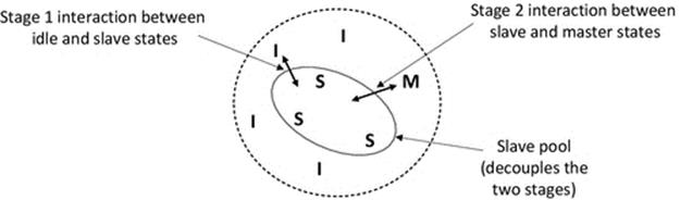
FIGURE 6.32 The two-stage operation of the Emergent Election Algorithm.
The first stage of the algorithm serves the purpose of enabling a very large population of processes to participate but most are passive at any time (i.e., they are in the idle state and do not send messages; they only listen).
The slave-master interaction occurs in the second stage of the algorithm and must be deterministic, that is, during an election, only a single slave can become master. This requires that the slaves have some means of negotiating between themselves. Slaves use timers to monitor the presence of the master by listening for its periodic heartbeat messages. When a master heartbeat is received, the timer is restarted, but if the end of the time period is reached without hearing from the master, the particular slave elevates to candidate status and broadcasts a candidate message. The candidate message informs slaves that the master has failed and also provides the address of the candidate. Higher-addressed slaves then also elevate to candidate status and transmit candidate messages. Lower-addressed slaves remain in the slave state. Candidate nodes that receive higher-addressed candidate messages withdraw their candidacy (they revert to slave status). Eventually, only the highest addressed candidate remains. It elevates to master status and the election is complete.
The corresponding state transition diagram for the Emergent Election Algorithm is shown in Figure 6.33.
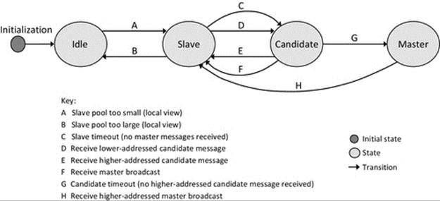
FIGURE 6.33 The state transition diagram for the Emergent Election Algorithm.
Activity D3
Exploring the Behavior of an Election Algorithm and Using an Automated Logging Tool
This activity uses the Emergent Election Algorithm that is built into the Distributed Systems Workbench. The activity explores the behavior of the election algorithm, in terms of the elections that occur, the state sequences of the individual instances, and the messages sent by those instances, under various conditions.
You will need at least two computers in the same local network to experiment with the election algorithm; only one copy will run on each computer because all instances use the same ports.
There is also an optional event logger utility that monitors all message events and state changes of the election algorithm processes and writes these to a logfile for subsequent analysis. The use of the logger is recommended for experiments where large numbers of election algorithm instances are used or where complex state change sequences are induced (e.g., by purposely starting additional instances in master state). The logger also uses the same ports as the election algorithm so it has to be run on an additional computer that does not have an instance of the election algorithm running.
Learning Outcomes
1. To gain experience of using an election algorithm.
2. To gain an appreciation of the behavior of an election algorithm.
3. To appreciate that a system may comprise a single process at the limit case and all behavioral rules must be respected in this case.
4. To gain an understanding of the mechanics of an election, including the state changes that occur at individual instances and the messages that are transmitted between instances.
5. To gain an appreciation of the usefulness of independent logging processes to capture dynamic event behavior in distributed applications.
Method Part A: Experimentation with a Single Instance of the Election Algorithm
The election algorithm should work correctly even if there is only one instance; this is the limit case (it is important to realize that the concept of a limit case also applies to other applications such as clock synchronization services, in which a single instance should “synchronize to itself”). The universal requirement for the election algorithm is that there should always be exactly one master, so a single instance should move to the master state and stay in that state.
Run the application called “Emergent Election Algorithm” from within the Distributed Systems Workbench on a single computer. Make sure the initial state is selected as “Idle” and press the Start button.
Expected Outcome for Part A
The screenshot below shows the election algorithm process; having started in the idle state, it has progressed through the other states in sequence to the master state. The process was left running and remained in the master state, which is the expected correct behavior.
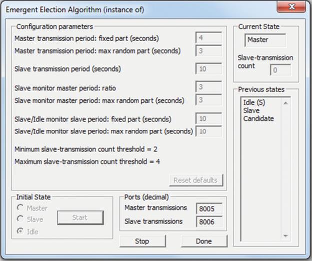
Method Part B: Use of a Logging Utility for Diagnostics
This part of the activity introduces a separate utility for logging the behavior of the election algorithm so that it can be analyzed precisely, later. This is very important when evaluating the algorithm in large systems or when gathering statistics, for example, in terms of efficiency measured as the number of messages per unit time, which is a measure of communication complexity and can impact scalability. To fully understand the internal behavior of the algorithm, it is important to capture the ordering of the events and key information such as which instances change from one particular state to another particular state.
In addition to the specific use of this logging utility, it is also intended that you gain an appreciation of the usefulness of independent logging processes to capture dynamic event behavior in distributed applications in the more general case. When complex scenarios arise, such as when many messages are being sent between components, or when there are large numbers of components, or when the relative timing of events is critical, then it is not possible to manually collate the information in a useful manner for subsequent analysis. The distributed nature of the system itself means that only by actually capturing the messages themselves can you identify the actual sequence of events and thus ensure correctness of the system or find complex timing-related problems.
First, create an empty logfile in a convenient location, for example, ElectionAlgorithm_Log.txt in the C:\temp directory (a simple editor such as Notepad can be used to create this file).
Once you have created the empty logfile, run the logger application called “Emergent Election Algorithm event logger” from within the Distributed Systems Workbench; this must be on a computer in the local network that is not running the election algorithm itself. Enter the path and filename of the logfile in the provided text box, and then press the “Start logging” button.
Expected Outcome for Part B
The screenshot on the left below shows the event logger running while a single instance of the election algorithm was running on another computer in the local network. You can see from the log trace that one election algorithm instance initialized in the idle state, and because it did not detect any messages from other instances, it elevated to slave state, then to candidate state, and then to master state. When in the slave state, it transmitted slave messages. Once in the master state, it transmitted master messages (these serve to prevent other instances elevating to candidate or master state).
The generated logfile content is shown on the right below. It shows the same information as the logger screen, as well as start time and the listening periods for master and slave messages (the periods over which messages are collated for logging and display purposes). The logfile is particularly useful for long-running experiments and for tracing sequences of node states when large numbers of nodes are used in experiments.
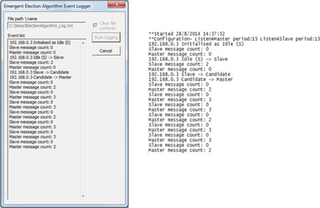
Method Part C: Experimentation with Multiple Instances of the Election Algorithm
The expected behavior is that an election occurs and a single instance enters the master state. A slave pool should be established with this particular algorithm; therefore, there should be between (typically) two and four slave state instances in larger systems. Additional instances should end up in the idle state.
Run multiple copies of the Emergent Election Algorithm each on separate computers (at least two computers are needed to perform this part adequately). Make sure the initial state in each case is selected as “Idle” and press the Start button.
Expected Outcome for Part C
One master instance was established (the user interface resembles the result for part A above). In my experiment, I only ran two instances, so the second instance settled in the slave state, which is the correct and expected behavior. The screenshot below shows the slave state process.
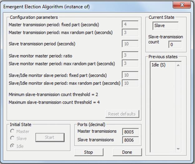
Method Part D: Stress Testing the Election Algorithm
Parts A and C above explored the election algorithm under stable conditions. However, in distributed systems, there can be highly dynamic, and unstable behavior where processes are started stopped or crashed unpredictably. This part of the activity explores the resilience of the election algorithm under some of these circumstances.
Experiment with a wide range of different starting conditions and interventions such as killing the master-state process or killing all the slave state processes and restarting them in the idle state.
Here is one particular experiment where the system is forced into an illegal state and left to recover:
Run multiple copies of the Emergent Election Algorithm each on separate computers. Let the system stabilize to where there is a single master.
Now, start one further instance of the election algorithm. In this case, make sure the initial state is selected as “Master” and press the Start button (thus creating a situation where there are two masters present).
Expected Outcome for Part D
Under any starting conditions and with any combination of starting and stopping instances and starting them in any state, the algorithm should work correctly and the system should settle to a steady state of one master, between two and four slaves and the remainder in the idle state. The screenshot below shows the behavior of a process that had previously elevated to master status. Another instance was started directly in master state, which is an illegal condition. This leads to a race in which the first master to hear a master message from the other will demote itself to slave status. In this case, the original master demoted (as can be seen in the screenshot, look at the previous state sequence and the current state) and the new instance stayed in master role.
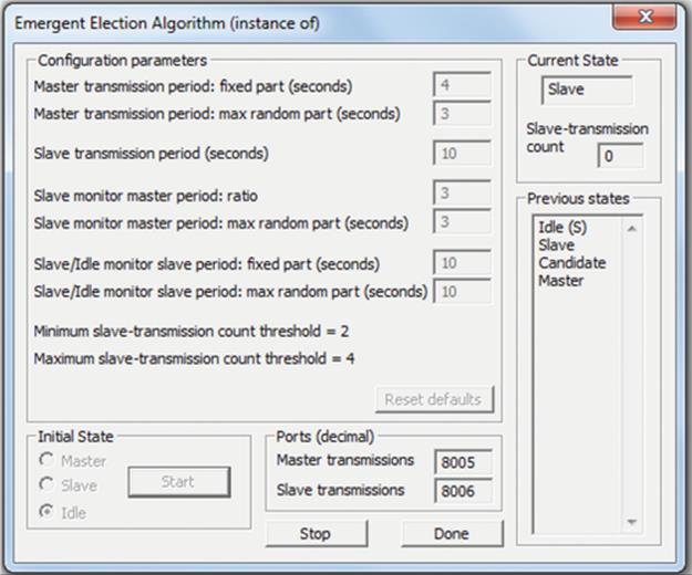
Reflection
This activity has explored the behavior of an election algorithm under a range of system conditions. It also introduced the use of automated logging utilities to capture the dynamic behavior of systems in a way that facilitates postmortem study of behavior and to check for correctness, enhance understanding, or identify problems.
Further Exploration
If you have access to a computer laboratory with moderate or large number of computers connected in the same broadcast domain (i.e., without separation by a router), try running the election algorithm on as many computers as you can.
Carry out some simple experiments to investigate characteristics of behavior such as the following:
• Does the number of process instances affect the time to reach a steady state?
• How many slave state instances are there on average? How steady is this value?
• What happens if you start ten or more instances in master state at the same time? (I found that by carefully positioning the keyboards, I can start four instances at the same time; use Tab to highlight the Start button and then you can start them all at once by simultaneously pressing the carriage return key. You can do at least two per person, so you may need a few helpers).
6.8 Group Communications
Many distributed applications require that processes work together in groups to solve particular problems or to provide a particular service. Externally, i.e., to their clients, these applications and services appear as a single process (this is a main transparency goal when designing such systems). However, internally, there can be complex behavior arising from the number of individual processes and the interactions between these processes. In particular, there need to be a means of control or coordination of the group and a means for messages from outside the group to be delivered to each member of the group in a way that is transparent to the external sender. In other words, the client should not need to identify the individual group members and send the message to each one in turn. In fact, the client should not need know the number of processes in the group or even that there are multiple processes.
Group communication mechanisms and protocols facilitate the maintenance of a group of processes that cooperate to perform some service. Typically, service groups will need to have dynamic membership, so that they can be scaled up and down as necessary to meet service demand. For example, consider a replicated database. The database servers may be organized as a group for the purpose of managing replication and ensuring consistency. Externally, a client may send an update request to the database service, unaware that internally within the group, an update propagation must take place. Only a single confirmation that the update has completed will be sent back to the client.
If the external interface to the group is by means of a group communication protocol, the client will see the same interface regardless of the number of processes in the group. The client should be unaware of internal complexities, for example, if additional servers are added when the request load increases or that some servers crash from time to time.
Group communication protocols can support a range of functionalities related to dynamic group maintenance and membership including
• group creation and destruction,
• process join and leave actions,
• send-to-group messaging,
• intra-group messaging.
There are two main approaches to group structure; hierarchical groups and peer groups, as illustrated in Figures 6.34 and 6.35, respectively.
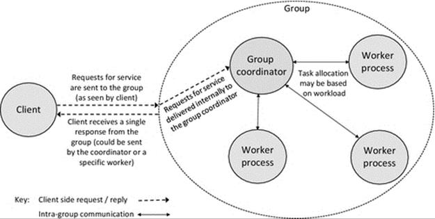
FIGURE 6.34 Hierarchical group structure.
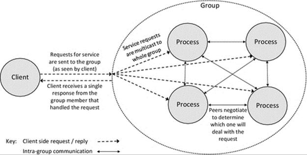
FIGURE 6.35 Peer group structure.
Figure 6.34 shows the structure of a hierarchical group, in which a coordinator process manages the group. The main role of the coordinator is to distribute service requests to the worker processes. The client is presented with a single-entity view of the group and the group-send method of the group communication protocol should hide details of the membership of the group and also the structure, so the client is unaware of the size of the group and the presence of the coordinator. The reply to a group-send message could be generated by the worker process that handled the request or by the coordinator.
The coordinator represents a single point of failure, and therefore, it may be necessary to implement an election algorithm (discussed earlier) to automatically select a replacement if the coordinator should fail.
Figure 6.35 shows the structure of a peer group, which by implication does not have a coordinator. Therefore, peers negotiate (or vote) to determine which one will deal with an incoming request. In some applications, this may be decided by the location of a specific resource (i.e., not all peers may be capable of providing the required service).
Peer groups are useful in dynamic and ad hoc applications. The difference between a peer-to-peer application and a peer group application is that in the former, the client is a peer (e.g., see the media sharing example and activity in Chapter 5). In the case of a peer group application, the peer group itself is a closed or bounded service and the client is an external entity. This has significant implications in terms of transparency, because the internal dynamic configuration of the peer group may be complex, but the client is shielded from it.
6.8.1 Transparency Aspects of Group Communication
For both types of groups, external clients of the group should be presented with a single-entity view of the group. Internally, groups can have complex structure and/or behavior, for example, the membership may change dynamically, processes may fail, and there may be a need to elect a new coordinator process. The fact that it is a group is known to the programmer, because messages are sent using primitives called, i.e., group-send or send-to-group. However, specific details of the group, such as group size, the identities of specific member processes, and the structure (whether or not there is a coordinator), are hidden from external processes.
6.9 Notification Services
There are many scenarios in distributed systems where a particular application (or process thereof) is concerned with knowing details of events that occur elsewhere in the system.
A notification service tracks events centrally and informs client applications when an event that is of interest to them occurs. For this to operate, the applications need to register with the notification service and provide details of which subset of events they are interested in. Such a service is most effective in systems where there are large numbers of events occurring (or that could occur) and individual clients are each only interested in a small subset of these. In contrast, if a process is interested in all (or a clear majority) of the events occurring, it may be more efficient for that process to monitor those events directly, removing the need for the notification service and the interaction with it.
Take, for example, automated stockbroking. A particular trading process may wish to buy shares in the company GlaxoSmithKline, but only if the price dips below 1200 pence per share, while another trading process may wish to sell shares in the same company, but only if the share price rises above 1600 pence per share. The actual market prices are held by a central brokerage system and change continuously throughout the day. As the prices can change quickly and dramatically and thus are not predictable, it is necessary for the trading processes to somehow keep track of the actual prices.
One option is for the brokerage system to continuously send out the prices of the stock, as they change. However, there are many thousands of different stocks listed on the exchange, and with price changes occurring at intervals of less than one second for many stocks, there are a lot of data to send out, and each trading process is only actually interested in a fraction of the information. This is quite inefficient and requires very high network bandwidth.
Another option is for the trading processes to repeatedly request the price of the particular stocks that they are interested in. This is called polling and would have to be done at a high rate to keep up with the fast price fluctuations that can occur. It is important to take into account that there can be a great many trading processes running simultaneously and each may be interested in a few tens or even hundreds of different stocks. Therefore, the polling approach could overwhelm the brokerage system or the communication network.
A more sophisticated approach for this situation would be to arrange that the trading processes register their interest in particular stocks, and the threshold prices they are waiting for, with a special notification service. This service would keep track of the stock prices, and whenever a prenotified target threshold is reached, the particular trading process would be notified. This approach cuts down on a lot of duplicate processing as each individual trading process is not continuously performing price comparisons, and also of course, there are significantly lower levels of network traffic.
6.9.1 Publish-Subscribe Services
Notification services can also be used as a form of middleware between processes within the same application. This is useful for applications where the various processes are each interested in certain subsets of events being generated by other processes. In such a scenario, the notification service is an example of what is called a publish-subscribe system; this is so named because some processes generate (publish) events that the notification service then forward to other processes that have preregistered their interest in (subscribed to) those events.
As an example, consider an online conferencing system with an integrated virtual whiteboard facility so that participants can draw diagrams to assist their discussions during a conference. Each user's computer has a local conferencing manager that manages the input and output resources of the system and maps these into a suitable user interface.
The conference manager registers with the notification service for the specific conferences that its user wishes to participate in; and for each of these conferences, it subscribes to the subset of events that the user requires (e.g., some users may have a voice-only interface and thus are not interested in the virtual whiteboard events).
Once the conference manager components have registered and subscribed to certain event types, the notification service will inform the managers when events of interest to them occur. Examples of events in this application include another user joining a conference and a user adding content to the virtual whiteboard. This scenario is illustrated in Figure 6.36.
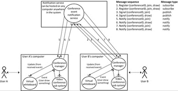
FIGURE 6.36 Notification service illustrated in the context of an online conferencing scenario.
Figure 6.36 shows the way in which a notification service decouples two application components such that they communicate indirectly. The notification service forwards only those events that each conferencing manager component has previously subscribed to, i.e., registered an interest in.
The figure shows the interaction taking place in the following sequence: steps 1 and 2; each conference manager registers with the conference event notification service. They each provide details of the actual conference, as well as the type of events within the conference that they are interested in. In this case, the event types are join events (when other users join the conference) and draw events (when existing conference members draw on the virtual whiteboard). User B then joins the conference and draws on the virtual whiteboard (steps 3 and 4, respectively). The notification service sees that both managers have subscribed to these event types, so each event is forwarded to each manager (steps 5, 6, 7, and 8).
The publish-subscribe mechanism is important because it decouples components both at the design time and at the runtime and therefore facilitates flexible dynamic configuration. A notification service provides loose coupling (because the relationships between different components are decided by runtime needs and thus not fixed at design time) and also provides indirect coupling (because the components only need to communicate with the intermediary, the notification service, and do not need to communicate directly with each other). There is an activity based on an event notification service in Chapter 7 (see also the detailed discussion on component coupling in Chapter 5).
6.10 Middleware: Mechanism and Operation
Middleware has been introduced in Chapter 5 in the form of an overview of its operation and a discussion of the ways in which middleware supports software architectures.
This section deals with the mechanistic and operational aspects of middleware and the ways in which it provides transparency to applications.
Middleware comprises the addition of a “middle” virtual layer between applications and the underlying platforms they run on. The layer is conceptually continuous across the entire system such that all processes sit above it and all platform resources are conceptually below it. By communicating through the layer, all aspects of location, the network, and computer boundaries are abstracted away (see Figure 6.37).
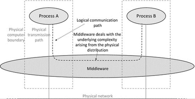
FIGURE 6.37 Middleware represented as a virtual layer connecting processes across the system.
Figure 6.37 provides an overview of the middleware concept. Processes communicate only via the middleware layer; they are not concerned with physical aspects of the system such as which platform they are running on or the addresses of other processes they are communicating with.
The virtual layer architecture of middleware provides significant transparency, in several of its forms, to processes. To achieve this, the middleware itself is quite complex internally. To achieve the illusion of the virtual layer, the middleware consists of processes and services located on each participating computer and special communication protocols connecting these components together so that collectively, they act like a continuous “layer” or “channel” that is spread across all computers. The middleware communication is typically based on top of TCP connections between the participating computers and may also use higher-level constructed forms of communication such as RMI to support remote method calls to application processes. The middleware hides differences in the underlying platforms from processes, but the middleware components must themselves be implemented specifically for their respective platforms and operating system. Figure 6.38 shows a physical system view of middleware.
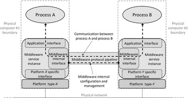
FIGURE 6.38 Middleware under the hood: a physical system view of middleware.
Figure 6.38 shows in a generic way the main internal components of middleware. There are three main types of interface that must be supported: (1) The application interface through which process-to-process communication is facilitated—Processes are given the illusion that they are sending messages directly to other processes, but actually, they send and receive messages to/from the middleware, which forwards the messages on to the other processes on their behalf, therefore providing location and access transparency. (2) The middleware internal interface through which the middleware components communicate and are managed—The various middleware service instances work together internally through a special protocol (which is defined by the middleware) to provide externally the illusion that the middleware is a single continuous layer, therefore achieving distribution transparency (the network is hidden). The middleware internal interface is used to pass control and configuration messages between middleware instances to maintain the middleware structure itself, as well as to forward messages from application components between parts of the system so that they reappear at the destination component's site as if the sender were a local process. (3) The platform-specific interface enables the middleware to work across a number of different platform types in the same system, therefore overcoming heterogeneity. This interface is the only part of the middleware that has to change to move the middleware across to a new platform; all of the middleware services and transparency provision are unchanged.
6.11 Middleware Examples and Support Technologies
6.11.1 The Common Object Request Broker Architecture (CORBA)
There are many types of middleware; CORBA is a standard defined by the Object Management Group (OMG) and is one of the best-known and historically most widely used examples. CORBA has been around since 1991 and is therefore considered to be a legacy technology by some practitioners, in some opinions superseded by other technologies such as Web services (see later). However, it still has many strengths and is still is in use.
CORBA serves as a useful reference model by which to explain some of the mechanics of middleware operation and some of the transparency aspects of middleware.
6.11.1.1 Motivation for CORBA
Distributed systems represent highly dynamic environments in which significant complexity stems from a wide variety of sources, some of which are inherent in the nature of distribution. Complexity challenges include a large location space in which it is necessary to find resources; communication latency; message loss; partial failures of networks; service partitioning (e.g., the functional split between client and server); replication, concurrency, and consistency control; and the requirement of consistent ordering of distributed events. In addition to these inherent forms of complexity, there are some accidental or avoidable forms of complexity that include the continuous rediscovery and reinvention of core concepts and components and lack of a single common design or development methodology. Distributed systems are also subject to various forms of heterogeneity that have been discussed in detail in Chapter 5.
CORBA was created as an answer to the problems of complexity and heterogeneity in distributed systems. With no consensus ever likely on hardware platforms, operating systems, programming languages, or application formats, the goal of CORBA was to facilitate universal interoperability. In this regard, CORBA allows application components to be accessed from anywhere in a network, regardless of the operating system they are running on and the language they are written in.
In CORBA systems, the communicating entities are objects (which are themselves part of larger applications). Dividing into separate entities at the object level allows for flexible fine-grained distribution of services, functionality, data resources, and workload, across the processing resources of the system.
The ORB is the central component of CORBA. An ORB provides mechanisms to invoke methods on local and remote objects, as illustrated in Figure 6.39.
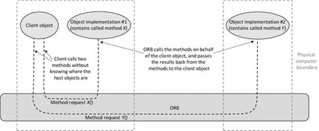
FIGURE 6.39 The object request broker provides a transparent connectivity service supporting method calls.
Figure 6.39 shows a simplified representation of a client object making two calls to methods on other objects, showing only the ORB aspects and not other components of the middleware. The client object does not know where the host objects of these methods (the implementation objects) are located. The figure shows that it does not matter whether the implementation objects are local or remote to the client; the ORB handles the method invocation transparently.
As indicated by the example in Figure 6.39, the ORB provides several forms of transparency. When an object (the client) makes a method request, the ORB automatically locates the host object and calls the requested method. The middleware layer hides platform and operating system heterogeneity that may be present when the called object is remote (the so-called object may be hosted on a physical platform of a different hardware type and/or running a different operating system to the client object's platform). The middleware uses a special IDL format when passing arguments to methods, which means that the objects can be written in different languages that use different call semantics; this will not affect the method call.
The transparency provided by the ORB (achieved with support from other components of CORBA) is summarized as follows:
• Access transparency. The calling object does not need to know if a called object is local or remote. Object methods are invoked in the same manner whether they are local or remote to the calling object.
• Location transparency. The location of a called object is not known and does not need to be known by the client object when invoking that object's methods. The called object does not need to know the location of the calling object when passing back results.
• Implementation transparency. Objects interoperate together despite possibly being written in different languages or residing in heterogeneous environments with different hardware platforms or operating systems.
• Distribution transparency. The communications network is hidden. The middleware takes care of setting up low-level (transport-layer) connections between the involved computers and manages all object-level communication using its own special protocols that sit above TCP. At the object-level, a single platform illusion is provided such that objects see all other objects as if they are local.
Figure 6.39 hides a lot of detail as to the actual architecture of CORBA and the actual mechanisms used to invoke method calls. In addition to the ORB, there are several other components and interfaces as shown in Figure 6.40.
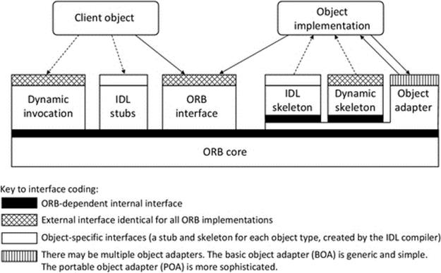
FIGURE 6.40 The ORB-related components and interfaces.
Figure 6.40 shows the architecture of CORBA, from the perspective of the ORB and its support components. Also shown are the various interfaces, which are in two categories: those between internal components and also the external interfaces to application objects. Two alternative forms of method invocation are supported—static and dynamic—which each involve different groups of components; the alternative paths are represented by the dotted arrows in the figure.
The subsections below provide details of the roles and behavior of the various components of CORBA and the interactions that occur between the components.
6.11.1.2 Object Adapter and Skeleton
An object adapter is a special component used to interface the CORBA mechanisms to an implementation object (i.e., an object on which a method is to be called). In addition to actually invoking the requested method, the object adapter performs some preparatory actions that include the following:
• Implementation activation and deactivation. The requested application component (the one hosting the object that contains the called method) may not be running (instantiated) when a request arrives to the ORB. If this were to happen in nonmiddleware-based applications in which a client component attempts to connect to a nonrunning server, the call would fail. With CORBA, there is an opportunity for the object adapter to actually instantiate the service component in such circumstances, prior to actually making the method request. It is also possible to leave the application component running after the method has been called or for the object adapter to deactivate it, depending on the server activation policy (see below).
• Mapping object references to implementations. A mapping of which object IDs are provided by each instantiated application component is maintained.
• Registration of implementations. A mapping of the physical location of instantiated application components is maintained.
• Generation and interpretation of object references. When a request to invoke a particular method is received, the ORB locates the particular service instance needed. It does this by relating together the mapping of the required object ID to an instantiation of a specific component and the mapping of instantiated components to locations.
• Object activation and deactivation. Once an object's service host component is instantiated, it may be necessary to separately instantiate specific objects (essentially by creating an instance of the object and calling its constructor).
Once all preparatory steps have been completed, the requested method is invoked (called), with the aid of the object's skeleton.
The skeleton is a server-side object-specific interface that actually performs the method invocation. The skeleton performs three functions: (1) It preserves the semantics of the object request and of the response, by translating the arguments from the IDL representation into the necessary object representation (which is dependent on the implementation language of the server object) and back into IDL for the response; (2) it makes the remote call appear as a local call from the point of view of the server object; (3) it takes care of the network connectivity aspects of the call so that the server application logic need not do so.
The combined operation of the object adapter and the skeleton is portrayed in an example application context in Figure 6.41.
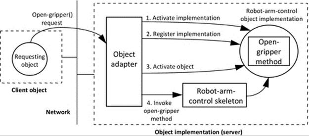
FIGURE 6.41 Object adapter management of method invocation.
Figure 6.41 illustrates the object adapter's management of method invocation, including the usage of the skeleton, placed into the context of a robot arm application example. In the scenario shown, the client object makes a request to open the robot arm's gripper, by calling the open-gripper method, without knowing the activation status of the server implementation component that hosts the object that contains this method. In the scenario, the server implementation is not already instantiated so the object adapter must first activate (instantiate) an instance of the application component that contains the Robot-Arm-Control object (step 1 in the figure). In step 2, the newly started component is now registered in a repository so that future service requests can be directed to it (otherwise, each new request could result in the instantiation of a dedicated component instance). In step 3, the Robot-Arm-Control object is activated (essentially, this means that an actual object instance of the appropriate class is created and its constructor called). In step 4, the open-gripper method is called using the precreated custom skeleton interface for the object (the skeleton actually performs a local method call on behalf of the remote client object). The server object responds by passing the result of the call back to the skeleton as though the skeleton were the client. This is an important aspect of distribution transparency from the application developer's viewpoint: the fact that the server object thinks it is being called locally means that no special communication considerations need to be made by the server's developer.
6.11.1.3 CORBA Object Servers and Activation Policy
There are several types of object server that can be implemented in CORBA, differentiated by the activation policy that describes the ways the object implementation and object activation are achieved. The different activation policies are as follows:
• Shared server policy. An object adapter activates a given server process the first time that one of its objects receives a request. The server then remains active. A server may implement multiple objects.
• Unshared server policy. The same as a shared server policy except that a server may implement only one object.
• Per-method server policy. Each method request causes a new server process to be started dynamically. Servers terminate once they have executed a method.
• Persistent server policy. Servers are initiated outside of the object adapter. The object adapter is still used to route method requests to the servers. In this situation, if a method request occurs for an object whose server is not already running, the call will fail.
6.11.1.4 CORBA's Repositories
CORBA uses two databases to keep track of the state of the system:
• The implementation repository is used by the ORB and object adapter to keep track of object servers and their runtime instances. In other words, it is a dynamic database of whether or not server applications are actually instantiated (running) and the location details of those that are running, so that requests can be forwarded to them.
• The interface repository is a database that contains descriptions of the methods associated with each class. Details are held in the form of IDL descriptions of each method's interface (which are programming language-independent). This database is used during dynamic method invocation to find a suitable server object for a dynamic request by matching the IDL definition of each of the server's method prototypes against the IDL description in the request message.
6.11.1.5 Static Method Invocation
Static invocation is used when the client object wants to send a request message to a specific design-time-known object. The mechanism of static invocation is illustrated in Figure 6.42.
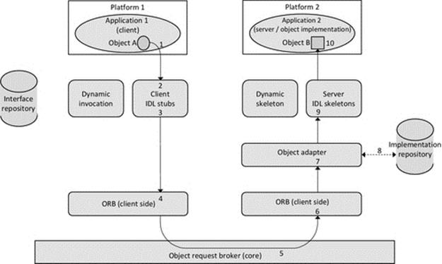
FIGURE 6.42 The mechanism of static method invocation.
Figure 6.42 illustrates how static invocation takes place. The sequence of steps shown in the figure begins at the point where a client identifies a particular implementation object that it wishes to send a method invocation request to. The steps are as follows:
1. The client object sends the request message.
2. The message is passed to the client stub (associated with the client object's application) that represents the server object (an application has one such stub for each remote object that it may access).
3. The message is converted into IDL representation.
4. The IDL code is passed via the client-side ORB (for the client platform) to the network. The client-side ORB consists of local services that the application may use (e.g., it may convert an object reference to a string for type-safe transmission over the network).
5. The message is passed over the network through the ORB core. CORBA enforces strict syntax and the mode of transport for messages passed over the network to ensure interoperability between CORBA implementations. The required syntax is the General Inter-ORB Protocol (GIOP) and the mode of transport is the Internet Inter-ORB Protocol (IIOP), which operates over TCP.
6. Once the message arrives at the server object's platform, it is picked up by the client-side ORB (which may perform local services such as object reference format conversion) and passed to the object adapter.
7. The object adapter provides the runtime environment for instantiating server objects and passing requests to them.
8. The object adapter searches the implementation repository to find an already running instance of the required server object or, otherwise, instantiates and registers the newly instantiated server object with the repository.
9. The object adapter passes the message to the appropriate server skeleton, which translates the IDL message into the message format of the specific server object.
10. The server object receives the message and acts on it.
6.11.1.6 Dynamic Method Invocation
Dynamic method invocation is used when the client object requests a service (by description) but does not know the specific object ID or class of object to satisfy the request. This supports runtime-configured applications where the relationships between components are not determined at design time, that is, components are not tightly coupled (see the discussion on component coupling in Chapter 5).
Figure 6.43 illustrates how dynamic method invocation takes place. The sequence of steps shown in the figure begins at the point where a client identifies a particular implementation object that it wishes to send a method invocation request to. The steps are as follows:
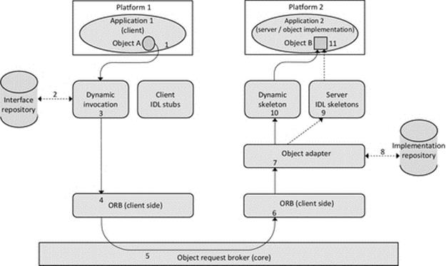
FIGURE 6.43 The mechanism of dynamic method invocation.
1. The client object sends the message to the dynamic method invocation utility.
2. The dynamic method invocation utility accesses an interface repository (a runtime database) that contains IDL descriptions of the methods associated with various objects. The dynamic method invocation utility identifies one or more objects that have methods that could satisfy the request.
3. The request is converted to IDL code and routed to those objects.
4. The IDL code is passed via the client-side ORB (for the client platform) to the network.
5. The message is passed over the network through the ORB core, using the GIOP and IIOP as with the static invocation mechanism.
6. The message is received by the client-side ORB (this time on the server-object's platform).
7. The message is passed via the object adapter to the appropriate object (which may need to be instantiated).
8. The object adapter searches the implementation repository to find an already running instance of the required server object or, otherwise, instantiates and registers the newly instantiated server object with the repository.
9. If the appropriate object on the server has an IDL skeleton, the message is passed via the server skeleton and thereby translated from IDL code into the message format of the target (server) object.
10. In the more complicated case, when the server object does not have an appropriate skeleton, the dynamic skeleton utility dynamically creates a skeleton for the server object and translates the IDL code into the message format of the target (server) object.
11. The server object receives the message and acts on it.
6.11.1.7 OMG Interface Definition Language (IDL)
The use of an IDL in middleware such as CORBA is a very powerful concept for application interoperability and in particular solves the problem of interoperability between objects written in different programming languages (and thus achieves implementation transparency). CORBA uses the OMG IDL, which is a specific instance of an IDL with support for several target languages including C, C++, and Java.
The OMG IDL is used to describe the interfaces to objects so that method calls can be made to them. IDL descriptions completely and unambiguously define all aspects of component call interfaces, including the parameters, their types, and the direction in which each parameter is passed (into the method or returned from the method). Using these interface definitions, a client component can make a method call on a remote object without knowing the language the remote object is written in and also without needing to know how the functionality is implemented; the IDL description does not include the internal behavior of the method.
The IDL interface definitions are needed during the automatic generation of the code (see below) in order that stubs and skeletons can automatically be generated and compiled into the application code. This removes the need for application developers to be concerned with communication and interoperability aspects and instead focus only on the business logic of components, as if all calls were between local objects.
See also the further discussion on IDL in a later section.
6.11.1.8 CORBA Application Development
Middleware such as CORBA provides design-time transparency to application developers and runtime transparency to applications and objects. The use of CORBA simplifies the application developer's role in building distributed applications because it facilitates interoperability between components and also provides mechanisms to take care of the networking and connectivity aspects.
The application development approach encouraged that developers write their code as if all components were to run locally and therefore not require any networking support. The developer must still take care of the separation of concerns and distribute the application logic across the components appropriately. Where there are static design-time-known relationships between components, these are built-in (this implies the use of the static invocation mechanism at runtime). So if, for example, a particular component Xis known to need to contact component Y to perform some specific function, then this relationship will be built into the application logic, in the same way as static relationships between objects are embedded in nondistributed applications.
The application developer must however perform an additional step, which is to describe the interfaces between the components using OMG IDL.
6.11.1.9 Automatic Code Generation in CORBA
The user-provided IDL code specifies the interfaces of objects and thus defines how their methods are invoked. Based on the IDL definitions, the IDL compiler generates the client stubs and server implementation skeletons.
The stub and skeleton provide an object-specific interface between the object and the ORB, as shown in Figure 6.40. Significantly, this removes the need for the application developer to write any communication code, and because of transparencies provided by the various CORBA components and mechanisms, the application developer does not need to be concerned with any aspects of distribution such as the relative locality or remoteness of objects and network addresses. The stubs and skeletons automatically include the necessary links between the objects and the CORBA mechanisms that deal with the actual network communication automatically.
The server implementation skeleton is used by the ORB and object adapter to make calls to method implementations. The IDL definitions provide the object adapter with the required format of each specific method call.
Figure 6.44 illustrates the basic sequence of steps in the development of CORBA applications. The developer's role is simplified because the complexity of the distribution, networking, and connectivity is handled automatically by CORBA's mechanisms that are driven by the IDL.
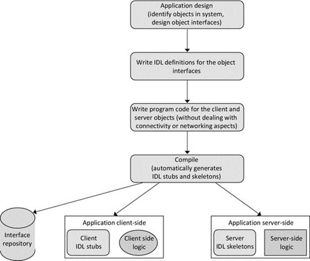
FIGURE 6.44 The sequence of steps to develop a CORBA application.
6.11.2 Interface Definition Language (IDL)
The IDL approach separates the interface part of program code from the implementation part. This is very significant for distributed systems because these are two types of concern that should ideally be treated in different ways. Application developers need to focus on the business logic aspects of application behavior (i.e., the implementation). The separation of interface from implementation facilitates automation of interface- related aspects such as connectivity and communication functionality, through middleware services.
There are various IDLs, used in specific middlewares, but they tend to be similar in terms of the role they perform, the ways in which they are used, and their syntax. CORBA uses the OMG IDL, for example, while Microsoft defined the Microsoft IDL (MIDL) primarily for use with its other technologies such as OLE, COM, and DCOM.
An IDL is designed to be programming language-independent, that is, it defines the interface of a component only in terms of the names of methods and the parameter types that are passed in and out of the method, regardless of whether the method is implemented in C++, C#, Java, or some other language. An IDL explicitly identifies the type and direction of each parameter. The type values supported are the same in general as most languages and include int, float, double, bool, and string. The direction is defined explicitly (as being an input to the method (in), an output from the method (out) or a parameter that is passed in and modified, and the new value output (in, out)) instead of implicit representation in which the position of the parameter in addition to the use of special symbols (such as * and &) indicates the way the parameters are used. An example of an (in, out) parameter in conventional C usage is a value passed into a method by reference, whereby the called method may modify the variable (this is the same instance of the variable that is visible to the calling method, so the change in value will be seen when the call returns). In addition to the basic description of parameters, IDL can provide additional constraints (such as maximum and minimum values). Figure 6.45puts the use of IDL into context with a simple example.
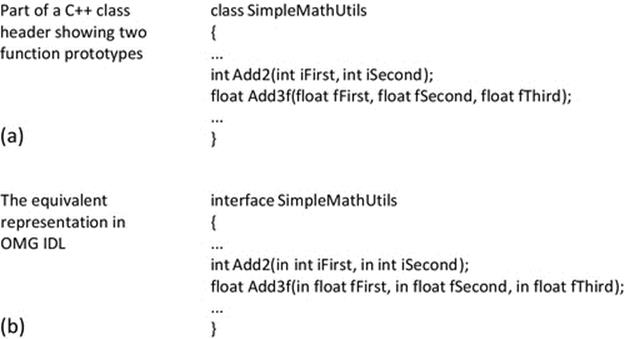
FIGURE 6.45 Comparison of programming language-specific interface definitions and IDL.
Figure 6.45 provides a very simple example of the OMG IDL syntax. Part A shows part of the C++ header file for a simple class called simple MathUtils. There are two simple member function declarations shown. Part B of the figure shows the equivalent OMG IDL representation. Notice that the IDL representation is quite similar to the C++ header file format; this is not surprising when you consider that the header file is essentially an interface specification and does not contain implementation detail. In the particular example shown (for C++), the IDL uses the term interface to replace class and places the parameter direction ahead of each listed parameter, to avoid any language-specific implied meaning. IDL does use implication in regard to the parameter to the left of the method name, which is implied to be an out parameter by its position (as with many high-level languages).
The implementation of the application logic is contained within the components themselves and is not exposed at its interfaces; therefore, IDL does not need to represent the implementation. So for the example shown in Figure 6.45, the IDL representation does not show how the addition methods work. This detail is not required by the calling component, which only needs the information shown in the interface definition in order to invoke the methods; for this reason, IDL does not have language constructs to represent the implementation.
The most significant difference between the two representations of the same interface in Figure 6.45 is that the C++ specific one is only understood by a C++ compiler, and therefore, only another component written in C++ could call the methods. The IDL representation can be used with any of the supported languages (which are many) so the fact that the simple MathUtils server object has been developed in C++ does not place any restrictions on the language used to develop a client object that calls its methods.
6.11.3 Extensible Markup Language
Extensible Markup Language (XML) is a standard, platform-independent markup language that defines format rules for encoding data. A main strength is that it provides an unambiguous way to represent structured data for use within applications, in particular as a format for storage and for communication in messages.
XML's portability across different platforms makes it ideal for representing data in distributed systems, overcoming heterogeneity. The XML is also extensible, which enables application-specific and application domain-specific variations of the basic language to be created, a classic example of which is the Chemical Markup Language (CML); this is used to describe complex molecular structures in a standardized and unambiguous document format. XML's characteristics have led to its popular use in many applications, as well as being the data representation method of choice in other protocols such as SOAP and Web services. A simple example of the use of XML to encode structured data is provided in Figure 6.46.
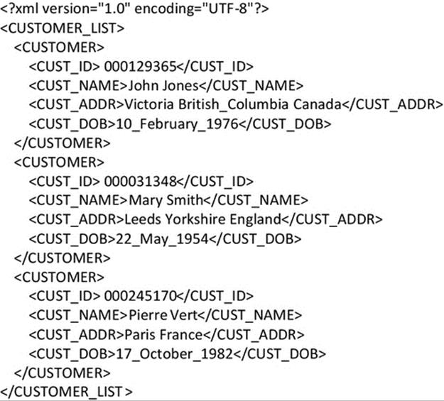
FIGURE 6.46 XML encoding in a simple application example.
Figure 6.46 illustrates how XML provides a simple way in which to encode complex data structures in an unambiguous way. The data representation format not only is easy to parse within a computer program but also is human-readable, which contributes to usability significantly. Compare, for example, with simpler formats that could be considered alternatives, such as a comma-separated file in which each data field is separated by a delimiter such as a comma and the position in the list denotes the meaning of each field; this is illustrated in Figure 6.47.
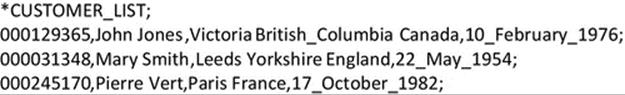
FIGURE 6.47 Comma-separated list format—for comparison with XML.
Figure 6.47 presents the same data as encoded in Figure 6.46, but in a simple comma-separated list format. In this example, the field delimiter is a comma and the row delimiter is a semicolon. The comma-separated list format serves to illustrate the relative benefits of XML. The comma-separated list format is more efficient, but XML has several advantages: (1) It preserves the structure of the data. (2) It names each field explicitly, which makes the format more readable. (3) It supports repetition of several data items of the same type within a single data record; for example, consider extending both the XML and comma-separated representations of the customer data to encode customers' phone numbers. The XML format can easily deal with situations where a customer has zero, one, or more phone numbers, because each entry is explicitly labeled. However, the comma-separated format uses position to represent meaning so repeating or omitted fields are not so simple to encode.
6.11.4 JavaScript Object Notation (JSON)
JSON is an efficient data-interchange format based on a subset of JavaScript and is both human-readable and straightforward for programs to create and parse. JSON is suitable for use in distributed systems because it uses a programming language-independent textual representation of data and thus provides implementation transparency in systems where multiple programming languages are used. JSON is a popular format for data interchange in Web applications.
A JSON script is organized in two levels. The outer level comprises a list of objects. Within this, each object is represented as a set of records, each expressed as an unordered list of name-value pairs delimited by commas. JSON is generally more concise than XML, a compromise between the simpler (raw) formats such as a comma-separated list and the highly structured XML. An application example of the JSON format is provided in Figure 6.48, using the same customer application as in Figures 6.46 and 6.47.
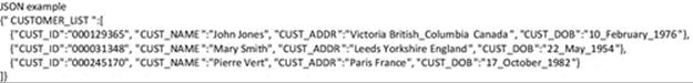
FIGURE 6.48 JSON encoding in a simple application example.
Figure 6.48 shows a JSON script that defines a single CUSTOMER_LIST object, which contains an array of 3 customer records. The example illustrates how JSON shares some efficiency characteristics with the comma-separated list format while also retaining the explicit labeling of XML, making it flexible with respect to the representation of complex data with repeating fields or omitted field values and enhancing human readability. The JSON usage of arrays and lists more naturally matches the data model used in most programming languages than XML does, and therefore, it is more efficient to parse.
6.11.5 Web Services and REST
A Web service is a communication interface that supports interoperability in distributed systems using standard Internet protocols used widely in the World Wide Web (Web) and as such is naturally platform-independent. The Web Services Description Language (WSDL) is used to describe the functionality of a Web service (WSDL is a type of IDL based on XML).
Clients communicate with the Web service using the Simple Object Access Protocol (SOAP), which is also a platform-independent standard (see later text). The SOAP messages themselves are encoded using XML and transmitted using the http, two further standards. The service is addressed using its URL, which describes the specific service and also represents the address of the host computer.
A main class of Web services is those that are REST-compliant. These Web services use a fixed set of operations—PUT (create), GET (read), POST (update), and DELETE—to manipulate XML representations of Web resources (see “Representational State Transfer (REST)” below). There are also arbitrary Web services, which are not constrained by the rules of REST and can thus expose an arbitrary set of operations. A simple example of a Web service application is shown in Figure 6.49.
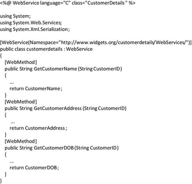
FIGURE 6.49 A simple Web service application example.
Figure 6.49 illustrates a simple Web service following the same Customer Details application scenario as the previous sections. The example shows a single stateless Web service with three GET methods {GetCustomerName, GetCustomerAddress, GetCustomerDOB}. The method requests are parameterized by the string value CustomerID. In other words, the Web service does not need to store any state concerning the client or the client's request; all the necessary information is self-contained in the request message. This is an important aspect that contributes to the scalability of Web services.
6.11.5.1 Representational State Transfer (REST)
REST is a set of guidelines that are designed to ensure high quality in applications such as Web services, in terms of simplicity, performance, and scalability. REST-compliant (or RESTful) Web services must have a client-server architecture and use a stateless communication protocol such as http.
The design of RESTful applications should respect the following four design principles:
1. Resource identification through URI: Resources that are accessible via a RESTful Web service should be identified by URIs. URIs represent a global Web-compliant-related address space.
2. Uniform interface: A fixed set of four operations—PUT, GET, POST, and DELETE—are provided to create, read, update, and delete resources, respectively. This restriction ensures clean, uncluttered, and universally understood interfaces.
3. Self-descriptive messages: Resources need to be represented in various formats, depending on the way they are to be manipulated and how their content is to be accessed. This requires that the representation of a resource in a message is decoupled from the actual resource itself and that the request and response messages identify the resource itself and either which operation is to be performed or the resulting value of the resource after the operation, respectively.
4. Stateful interactions through hyperlinks: The Web service itself, and thus each server-side interaction with a resource, should be stateless. This requires that request messages must be self-contained (i.e., the request message must contain sufficient information to contextualize the request so that it can be satisfied by the service without the need for any additional server-side-stored state concerning the client or its specific request).
6.11.6 The Simple Object Access Protocol (SOAP)
The SOAP facilitates connectivity in heterogeneous systems and is used to exchange structured information in Web services. It uses several standard Internet protocols to achieve platform and operating system-independent message transmission and message content representation. Message transmission is usually based on either hypertext transfer protocol (http) or Simple Mail Transfer Protocol (SMTP).
http and the XML are used to achieve information exchange in a format that is both universally recognized and unambiguous in interpretation. SOAP defines how an http header and an XML file should be encoded to create a request message and the corresponding response message so that components of distributed applications can communicate. Figure 6.50 illustrates the use of SOAP with a simple application example.
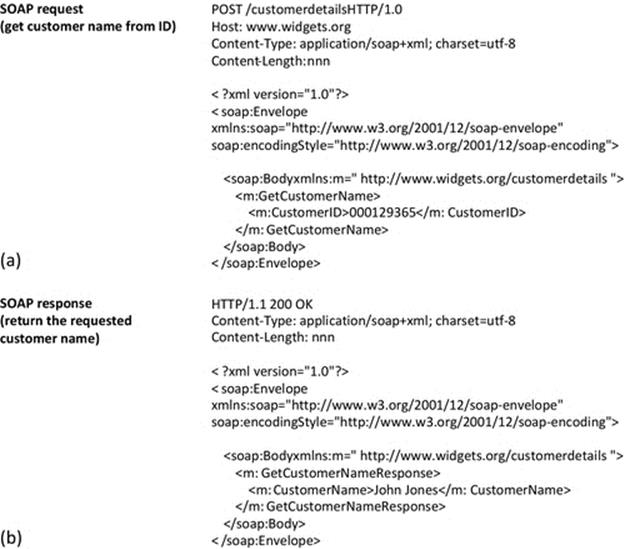
FIGURE 6.50 SOAP encoding in a simple application example.
Figure 6.50 provides a simple application example to illustrate the way in which SOAP combines HTML and XML to define unambiguous request and response message formats. Part A of the figure shows the SOAP request to get the name of a customer, based on a provided customer ID value. This is an http POST request type. Within the message, XML coding format is used to represent the structure of the request message data. Part B of the figure shows the corresponding response message.
6.12 Deterministic and Nondeterministic Aspects of Distributed Systems
Deterministic behavior essentially means predictable. If we know the initial conditions of a deterministic function, we can predict the outcome, whether it be a behavior or the result of a calculation.
Nondeterministic behavior arises in systems in which there are sufficient numbers of interacting components and sources of randomness that it is not possible to predict the future states precisely. Natural systems tend to be nondeterministic; examples include behavior in insect colonies, weather systems, and species population sizes. Human-oriented nondeterministic system examples include economies and crowd behavior. These systems are sensitive to their starting conditions and the actual sequences of interactions that occur within the system and possibly even the timing of those interactions. For such systems, it is usually possible to predict an expected range of outcomes, with varying confidence levels, rather than a knowable particular outcome. Computer simulations of nondeterministic systems may have to be run many times in order to gain usable results, with each run having slightly different starting conditions and yielding one possible outcome. Patterns in the set of outcomes may be used to predict the most likely of many possible futures.
For example, a weather forecasting algorithm is very complex and uses a large data set as its starting point in order to forecast a weather sequence. It is actually a simulation, computing a sequence of future states based on current and recent conditions. There may be some tuning parameters that affect the algorithm's sensitivity to certain characteristics of the input data. As there are so many factors affecting the accuracy of the weather forecast and also the fact that we cannot capture all the possible data needed with equal accuracy across all samples (sensors and/or their placement may be imperfect), there is always an element of error in the result. If we run the simulation just once, we may get a very good forecast, but it may also be poor (because of the varying sensitivity to specific weather histories and varying extents of dynamism in the weather systems). So although we may have the best forecast we are going to get, we cannot be confident that that is the case. If we change the tuning parameters very slightly and run the simulation again, we may get a similar or distinctly different result. Running the simulation many times with slightly different settings will give us a large number of outcomes, but hopefully, they are clustered together such that if somehow averaged, they provide a good approximation of what the weather will actually do. This is an example of a nondeterministic computation that hopefully yields a valuable result.
Distributed computer systems are themselves complex systems with many interacting parts. Nondeterministic behavior arises due to a large number of unpredictable characteristics of systems. For example, network traffic levels are continuously fluctuating, and this leads to different queue lengths building up, which in turn affects the delay to packets and also the probability of packets being dropped because a queue is full. Even a single hardware component can contribute nondeterministic behavior; consider the operation of a hard disk. Disk seek time is dependent on the rotation delay, which depends on where the disk is (in an angular sense) at the point of starting the seek and also the relative distance between the current track and one the head has to move to. These variations in starting conditions affect every block read from the disk so it is more likely that disk read times will vary each time than they will be exactly the same. The runtime of even a simple process depends on the sequence of low-level scheduling decisions made by the operating system, which in turn depend on the set of other processes present and the behavior of those processes. Therefore, executing a single process multiple times can lead to different runtimes, arising from the combination of differences in scheduling decisions, disk access latency, and communication latency.
The message for designers and developers of distributed applications and systems is that even if your algorithms are entirely deterministic in their operation and even if your data are complete and accurate, the underlying computing systems and networks are not perfect and not perfectly predictable. A component failure can happen at any time, a network message can be corrupted, the load on a processing host computer can change suddenly leading to increased latency of service, and so on. Seeking to eradicate all unpredictable behavior is futile, and the assumption of determinism is dangerous. You cannot prevent certain types of faults, and you cannot in general predict them. Instead, focus your design effort on making applications robust and fault-tolerant.
6.13 End of Chapter Exercises
6.13.1 Questions
Q1. Scalability and interaction complexity
(a) What is the level of interaction complexity in a system in which each component interacts with approximately half of the other components in the system?
(b) What is the formula for calculating the number of separate interactions that occur?
(c) How many separate interactions occur if there are 10 components in the system?
(d) How many separate interactions occur if there are 50 components in the system?
(e) How many separate interactions occur if there are 100 components in the system?
Q2. Scalability and interaction complexity
(a) What is the level of interaction complexity in a system in which each component interacts with approximately four other components in the system?
(b) What is the formula for calculating the number of separate interactions that occur?
(c) How many separate interactions occur if there are 10 components in the system?
(d) How many separate interactions occur if there are 50 components in the system?
(e) How many separate interactions occur if there are 100 components in the system?
Q3. Scalability
Comment on the relative scalability of the two systems described in questions 1 and 2.
Q4. Implementation transparency
(a) How does IDL contribute to implementation transparency?
(b) Why does IDL contain only interface definitions and not implementation detail?
Q5. Concurrency transparency
(a) What is the main challenge when facilitating concurrent access to shared resources?
(b) How do transactions contribute to concurrency transparency?
Q6. Location transparency
(a) Why is location transparency one of the most common requirements of distributed applications?
(b) How does a name service contribute to the achievement of location transparency?
Q7. Replication transparency
(a) What are the main motivations for replication of data and/or services?
(b) What is the main challenge when implementing replication?
(c) How does the two-phase commit protocol contribute to the achievement of robust replication mechanisms?
6.13.2 Programming Exercises
Programming Exercise #D1: This programming challenge relates to the use of directory services to provide location transparency. In particular, it involves the use of the directory service used in activity D1 (which is built into the Distributed Systems Workbench).
The task: Modify the client and server components of the use-case game so that the server can be registered with the directory service and the client can subsequently use the directory service to obtain the IP address and port details of the game server:
• For the server side: You need to consider at what point the game server is registered with the name service. This is best done automatically during the game server initialization.
• For the client side: There are two ways you could do this—you could have a button “contact directory service” on the client user interface; alternatively, a more transparent approach is for the client to contact the directory service automatically when the game client is started.
Note: the directory service can be run from within the Distributed Systems Workbench.
The interface to the directory service is defined as follows:
Protocol
UDP
Port number allocations
From_DIRECTORY_SERVICE_PORT 8002The port the application client must listen on for DirectoryServiceReply messages sent in response to RESOLVE request messages.
To_DIRECTORY_SERVICE_PORT 8008The port that application clients use to send RESOLVE messages to the directory service (broadcast is used).
The port that application servers use to send REGISTER messages to the directory service (broadcast is used).
Message Structures
The message structure returned by the directory service in response to RESOLVE request messages is shown in Figure 6.51.
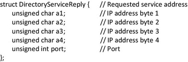
FIGURE 6.51 The directory service reply message format.
Message Formats
Client RESOLVE request messages are encoded as a character string containing “RESOLVE:server_name” where server_name can be a maximum of 30 characters. An example is RESOLVE:GameServer.
Server REGISTER messages are encoded as a character string containing “REGISTER:server_name:port” where server_name can be a maximum of 30 characters and the port number is expressed in text form. An example is REGISTER:GameServer:8004.
Note that for both message types, the IP address of the sending process is extracted by the directory service, directly from the header of the received message; the game component does not have to explicitly send it.
An example solution is provided in the programs: CaseStudyGame_Client_DS and CaseStudyGame_Server_DS.
Programming Exercise #D2: This programming challenge relates to the use of election algorithms to provide robustness and failure transparency. In particular, it is related to the election algorithm activity D3.
The task: Implement the bully election algorithm.
The operation of the bully election algorithm has been discussed earlier in the chapter, the most important aspect of behavior being that there must only be one master-state instance present at any time. Here are some specific implementation details for guidance:
1. Assume that the elections will occur between processes in a local network, and therefore, broadcast communication can be used.
2. Assume that only one participating process will be present on each computer, and therefore, the IP address of the host computer can be used as the process' ID for the purposes of the election (as this is a simple way to ensure that IDs are unique).
An example solution is provided in the program BullyElectionAlgorithm.
6.13.3 Answers to End of Chapter Questions
Q1. (Answer)
(a) Each of N components interacts with N/2 components, so interaction complexity is O(N*N/2).
(b) The formula for the number of separate interactions is N*N/4. The number of interactions is half of the interaction intensity because each interaction involves two components.
(c) If there are 10 components in the system, there are 25 separate interactions.
(d) If there are 50 components in the system, there are 625 separate interactions.
(e) If there are 100 components in the system, there are 2500 separate interactions.
Q2. (Answer)
(a) Each of N components interacts with 4 components, so interaction complexity is O(4N).
(b) The formula for the number of separate interactions is 2N. The number of interactions is half of the interaction intensity because each interaction involves two components.
(c) If there are 10 components in the system, there are 20 separate interactions.
(d) If there are 50 components in the system, there are 100 separate interactions.
(e) If there are 100 components in the system, there are 200 separate interactions.
Q3. (Answer)
The system described in question 1 has a steep exponential interaction complexity, which potentially has a severe impact on scalability. The system described in question 2 has a linear interaction complexity and therefore is more scalable.
Q4. (Answer)
(a) IDL facilitates interoperability when components are developed using different programming languages. It does this by providing a universal intermediate representation of method call interfaces, which is language-independent.
(b) IDL only needs to represent call requests in a language-independent way and thus is only concerned with component interfaces. IDL does not define the behavior or internal logic of the communicating components, so there is no need for IDL to express any implementation detail.
Q5. (Answer)
(a) The main challenge is maintaining consistency.
(b) Transactions prevent overlapped access to shared resources. The properties of atomicity, consistency, isolation, and durability collectively ensure that the system is left in a consistent state after each access and/or update event has completed.
Q6. (Answer)
(a) Components need to communicate with other components regardless of where they are located. There needs to be either an automated way to find the location of a component or alternatively a means of sending a message to another component through an intermediate service without the sender knowing the location of that component.
(b) A name service resolves a component name (or a resource name) into its address. Therefore, the sender of a message only needs to initially know the identity of the target component and not where it is located.
Q7. (Answer)
(a) Replication of data and/or services contributes to robustness, availability, responsiveness, and scalability.
(b) Replication involves creating multiple copies of data resources and state information. This introduces the potential for the different instances of a replicated resource to become inconsistent. Therefore, maintaining consistency is the main challenge when implementing replication.
(c) The two-phase commit protocol ensures that updates are performed at all replica instances of a data resource or at none of them, thus maintaining consistency.
6.13.4 List of In-Text Activities
|
Activity number |
Section |
Description |
|
D1 |
6.4.2 |
Experimentation with a Directory Service |
|
D2 |
6.5.7 |
Exploring address resolution and the gethostbyname DNS resolver |
|
D3 |
6.7.5 |
Exploring the behavior of an election algorithm and using an automated logging tool |
6.13.5 List of Accompanying Resources
The following resources are referred to directly in the chapter text, the in-text activities, and/or the end of chapter exercises:
• Distributed Systems Workbench (“Systems Programming” edition)
• Source code
• Executable code
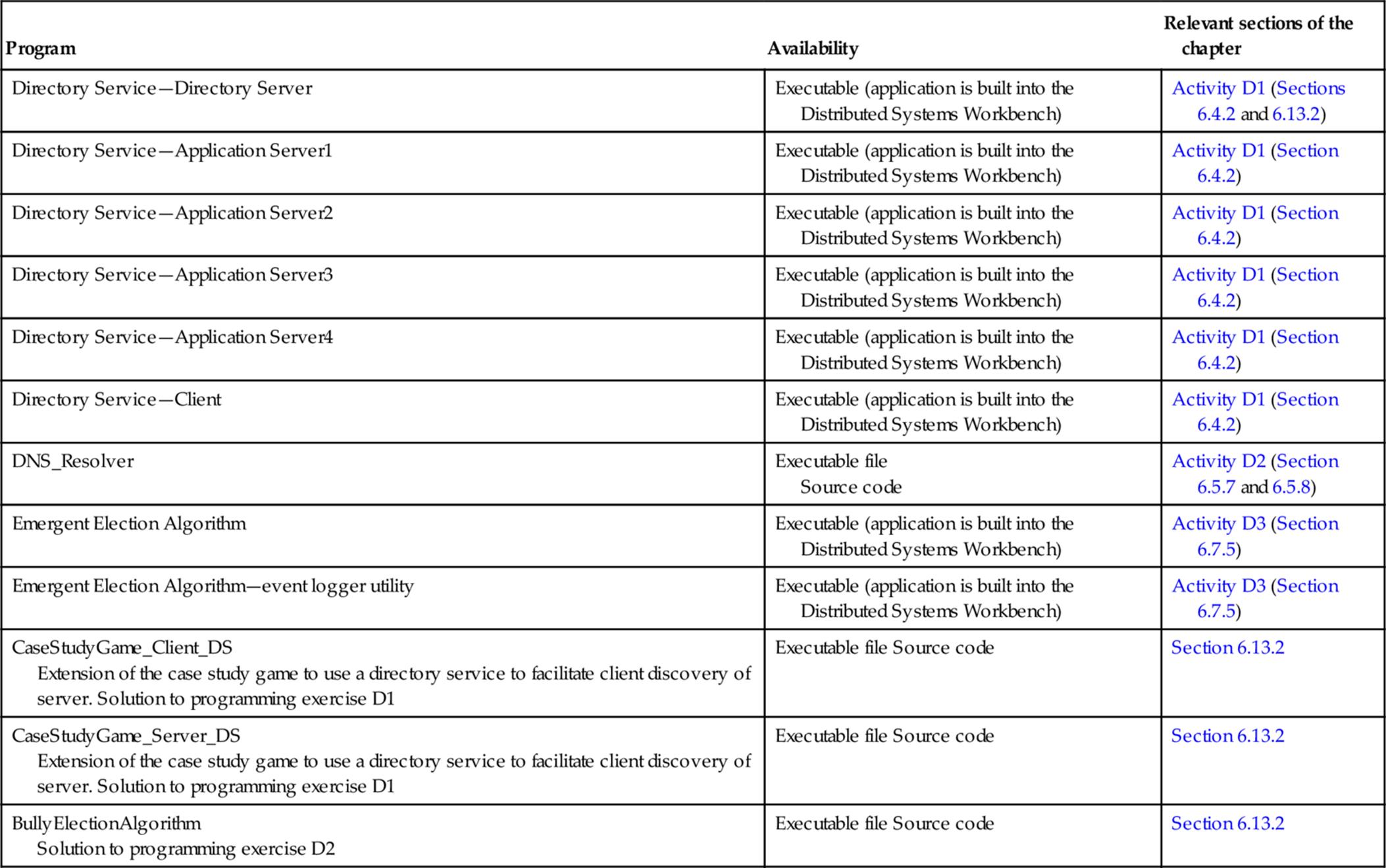
1 The DNS_Resolver example application used in this activity is written in C++ and uses the gethostbyname method. For C#, there is the equivalent Dns.GetHostByName method or Dns.GetHostEntry method, both of which are part of the.net framework. For Java, see the various methods of the java.net.InetAddress class, including getAllByName and getLocalHost.