Cython (2015)

Chapter 11. Cython in Practice: Spectral Norm

The competent programmer is fully aware of the strictly limited size of his own skull; therefore he approaches the programming task in full humility, and among other things he avoids clever tricks like the plague.

— E. Dijkstra

Like Chapter 4, this chapter’s intent is to reiterate concepts and techniques to show Cython’s use in context. Here we focus on using typed memoryviews to compute the spectral norm of a particular matrix. This is another example from the computer language benchmarks game, allowing us to compare the Cython solution’s performance to other highly optimized implementations in different languages. The focus here is how to use typed memoryviews to achieve much better performance with array-heavy operations. That said, we will first cover what the spectral norm is and explore a pure-Python version before using Cython to speed it up.

Overview of the Spectral Norm Python Code

The spectral norm of a matrix is defined to be the largest singular value of ; that is, the square root of the largest eigenvalue of the matrix , where is the conjugate transpose of . The spectral norm of a matrix is an important quantity that frequently arises, and it is often computed in computational linear algebra contexts.

To compute the spectral norm, we make use of one observation about : if the vector is parallel to the principal eigenvector of , then the quantity is identical to the spectral norm of . Therefore, if we compute for positive integer and random (nonzero) vector , each application of will align more closely with the principal eigenvector. This provides an iterative solution to compute the spectral norm, and at its core it uses a matrix-vector multiply.

The particular matrix for which we will compute the spectral norm is defined as:

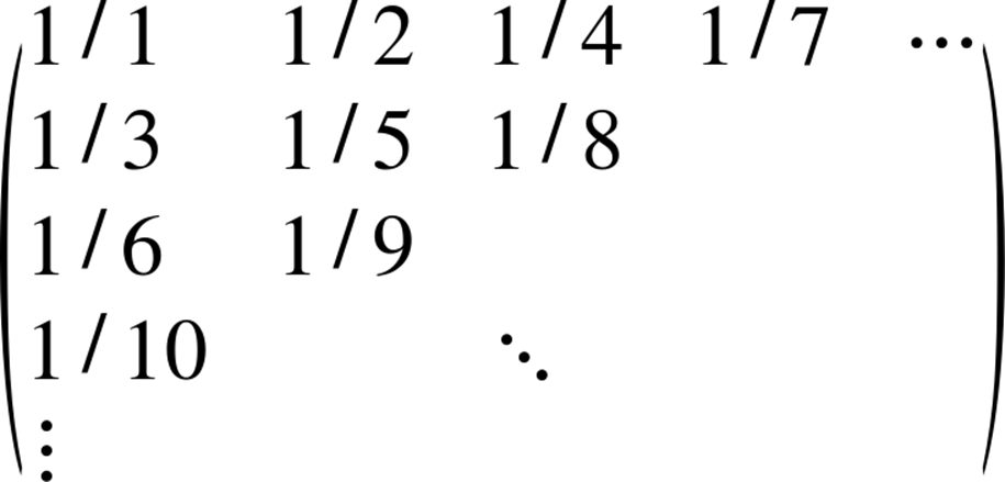
Given row i and column j—both zero-based—we can compute in a single expression:^[21^]

def A(i, j):

return 1.0 / (((i + j) * (i + j + 1) >> 1) + i + 1)

Alternatively, we could compute up to a given maximum number of rows and columns and store the result in a two-dimensional array. Because the matrix is dense, the memory required to store it grows very quickly. For more direct comparison with the other language implementations, we will use the computed version defined in the preceding code block.

The core of the program computes or :

def A_times_u(u, v):

u_len = len(u)

for i inrange(u_len):

partial_sum = 0.0

for j inrange(u_len):

partial_sum += A(i, j) * u[j]

v[i] = partial_sum

The definition of At_times_u is identical except for the partial_sum update:

def At_times_u(u, v):

# ...

for ...:

for ...:

partial_sum += A(j, i) * u[j]

# ...

To compute , we can first compute using A_times_u and then compute using At_times_u. That is what B_times_u does:

def B_times_u(u, out, tmp):

A_times_u(u, tmp)

At_times_u(tmp, out)

Because is an infinite matrix, some approximation must be used. The spectral norm program takes an integer n from the command line that determines the number of rows and columns in . It then creates an input vector u of length n initialized to 1, using the standard library array type:

def spectral_norm(n):

u = array("d", [1.0] * n)

v = array("d", [0.0] * n)

tmp = array("d", [0.0] * n)

Here, u is the input vector; v and tmp are intermediates.

The core of the program calls B_times_u a net 20 times, all while managing the temporaries to handle swapping values:

def spectral_norm(n):

# ...

for _ inrange(10):

B_times_u(u, v, tmp)

B_times_u(v, u, tmp)

After this loop is finished, the vectors u and v are both closely aligned with the principal eigenvector of B. The vector u has had one more application of B than v, so to compute the spectral norm of A, we compute , which is equivalent to :

def spectral_norm(n):

# ...

vBv = vv = 0

for ue, ve inzip(u, v):

vBv += ue * ve

vv += ve * ve

The spectral norm is then a simple expression, which we return:

def spectral_norm(n):

# ...

return sqrt(vBv / vv)

Altogether, the entire script is about 70 lines of code. The pure-Python version is (subjectively) one of the easier implementations to understand among all submitted versions, but it is also consistently orders of magnitude slower than many other implementations. Cython is ideally suited to allow the Python version to keep its expressiveness and improve its performance to be competitive.

Performance Profiling

Our pure-Python version is in a source file named spectral_norm.py. If run as a script from the command line, it will pass the input argument to spectral_norm and print the result:

if __name__ == "__main__":

n = int(sys.argv[1])

spec_norm = spectral_norm(n)

print("%0.9f" % spec_norm)

Let’s try it out for small inputs:

$ python ./spectral_norm.py 10

1.271844019

$ python ./spectral_norm.py 50

1.274193837

$ python ./spectral_norm.py 100

1.274219991

$ python ./spectral_norm.py 200

1.274223601

The true solution to 10 significant digits is 1.274224152, so as n increases, we see that the accuracy of the computed spectral norm improves as well.

Let’s run spectral_norm.py under a profiler (see Chapter 9) to see what occupies the runtime:

$ ipython --no-banner

In [1]: %run -p ./spectral_norm.py 300

3600154 function calls in 3.836 seconds

Ordered by: internal time

ncalls tottime percall cumtime percall filename:lineno(function)

3600000 1.826 0.000 1.826 0.000 spectral_norm.py:15(A)

20 1.013 0.051 1.934 0.097 spectral_norm.py:18(A_times_u)

20 0.995 0.050 1.900 0.095 spectral_norm.py:32(At_times_u)

1 0.000 0.000 3.835 3.835 spectral_norm.py:50(spectral_norm)

...

The column to focus on is tottime, which indicates the time spent in this function excluding time spent in called functions. Looking at the first three rows in the tottime column, we can conclude that the three functions A, A_times_u, and At_times_u together consume greater than 95 percent of the total runtime.

Cythonizing Our Code

With profiling data in hand, we can sketch out how we will use Cython to improve performance.

Before starting, first we rename spectral_norm.py to spectral_norm.pyx; this is the source of our Cython-generated extension module. We also create a minimal run_spec_norm.py driver script:

import sys

from spectral_norm import spectral_norm

print("%0.9f" % spectral_norm(int(sys.argv[1])))

We modify spectral_norm.pyx to work with this driver script, removing the if __name__ ... block.

We also need a setup.py script to compile spectral_norm.pyx:

from distutils.core import setup

from Cython.Build import cythonize

setup(name='spectral_norm',

ext_modules = cythonize('spectral_norm.pyx'))

Let’s compile and run our Cythonized version before doing anything else, to see what Cython can do unaided:

$ python setup.py build_ext -i

Compiling spectral_norm.pyx because it changed.

Cythonizing spectral_norm.pyx

running build_ext

building 'spectral_norm' extension

creating build

creating build/temp.macosx-10.4-x86_64-2.7

gcc -fno-strict-aliasing -fno-common -dynamic -g -O2

-DNDEBUG -g -fwrapv -O3 -Wall -Wstrict-prototypes

-I[...] -c spectral_norm.c -o [...]/spectral_norm.o

gcc -bundle -undefined dynamic_lookup

[...]/spectral_norm.o -o [...]/spectral_norm.so

Again, this output is specific for OS X. Consult Chapter 2 for platform-specific options to pass when compiling using distutils.

Now that all the infrastructure is in place, running our program is straightforward.

First, let’s see the runtime of our pure-Python version for comparison:

$ time python spectral_norm.py 300

1.274223986

python spectral_norm.py 300 3.14s user 0.01s system 99% cpu 3.152 total

The Cythonized version’s performance may be surprising:

$ time python run_spec_norm.py 300

1.274223986

python run_spec_norm.py 300 1.10s user 0.01s system 99% cpu 1.111 total

Remarkably, for this spectral norm calculation Cython is able to improve performance by nearly a factor of three, with no modifications to the core algorithm. This is a great start, and using more Cython features will only improve performance.

Adding Static Type Information

The A(i, j) function is called millions of times, so improving its performance will yield a significant payoff. It takes integer arguments and computes a floating-point value in a single expression, so converting it to use static typing is straightforward. By converting it to a cdef inlinefunction, we remove all Python overhead:

cdef inline double A(int i, int j):

return 1.0 / (((i + j) * (i + j + 1) >> 1) + i + 1)

Using Cython’s annotation support (see Chapter 9; output not shown here), we see that the body of A is still yellow. This is due to the division operation, which by default will raise a ZeroDivisionError if the denominator is zero. We already know that it is impossible for the denominator to be zero, so this check is unnecessary. Cython allows us to trade safety for performance by using the cdivision decorator to turn off the test for a zero denominator:

from cython cimport cdivison

@cdivison(True)

cdef inline double A(...):

# ...

After compiling again, we see that our optimized A function leads to another factor-of-two performance improvement:

$ time python run_spec_norm.py 300

1.274223986

python run_spec_norm.py 300 0.51s user 0.01s system 99% cpu 0.520 total

But we can do even better—let’s look at the matrix-vector multiplication functions.

Using Typed Memoryviews

The A_times_u and At_times_u functions work extensively with arrays inside nested for loops. This pattern is ideally suited to the use of typed memoryviews, covered in Chapter 10.

First we convert the untyped arguments of A_times_u to use one-dimensional contiguous typed memoryviews of dtype double:

def A_times_u(double[::1] u, double[::1] v):

# ...

We then provide static typing information for all internal variables:

def A_times_u(double[::1] u, double[::1] v):

cdef int i, j, u_len = len(u)

cdef double partial_sum

# ...

The body of A_times_u remains unmodified:

def A_times_u(double[::1] u, double[::1] v):

# ...

for i inrange(u_len):

partial_sum = 0.0

for j inrange(u_len):

partial_sum += A(i, j) * u[j]

v[i] = partial_sum

We make sure to provide static typing for all variables in the code body. Ensuring that u and v are contiguous typed memoryviews allows Cython to generate efficient indexing code for the innermost loop.

The At_times_u transformation is identical.

We leave both the B_times_u and spectral_norm functions unmodified. If you recall from our profiling run, the A, A_times_u, and At_times_u functions occupy more than 95 percent of the runtime. Modifying these functions to use Cython data structures and static types makes sense, but using Cython-specific features everywhere is not necessary and is an exercise in diminishing returns.

Because we use typed memoryviews for the u and v arguments, we can call the A_times_u and At_times_u functions with any Python object that supports the buffer protocol. So, whenever B_times_u calls A_times_u and At_times_u, the u and v typed memoryviews will acquire the underlying buffer from the provided array.array objects. They do so without copying data.

In Python 2, there is one more step to ensure array.array objects work with typed memoryviews. Near the top of the file, we add another compile-time import:

from cpython.array cimport array

After compiling with our Cythonized matrix-vector multiplication routines in place, we see that the runtime is now significantly faster than before:

$ time python run_spec_norm.py 300

1.274223986

python run_spec_norm.py 300 0.05s user 0.01s system 97% cpu 0.058 total

Using typed memoryviews and statically typing all inner variables in A_times_u and At_times_u has led to an additional factor-of-10 performance improvement.

As we saw in Chapter 10, we can generate slightly more efficient code inside A_times_u and At_times_u by turning off bounds checking and wraparound index checking:

from cython cimport boundscheck, wraparound

@boundscheck(False)

@wraparound(False)

cdef void A_times_u(...):

# ...

Perhaps unexpectedly, these optimizations do not affect performance by any measurable margin.

Comparing to the C Implementation

We are using the same algorithm here as is used in all the other solutions to the computer benchmark game, which allows us to compare Cython’s performance to C directly.

All C versions of the benchmark—including the serial version we compare to here—are freely available. We can compile and run the C version with an n of 5500, making sure to use the same optimization flags that we used for Python to ensure a fair comparison:

$ time ./spectralnorm.x 5500

1.274224153

./spectralnorm.x 5500 9.60s user 0.00s system 99% cpu 9.601 total

Our Cython version with n of 5500 run has identical output and identical performance (within measurement error):

$ time python run_spec_norm.py 5500

1.274224153

python run_spec_norm.py 5500 9.61s user 0.01s system 99% cpu 9.621 total

The fastest C implementation makes use of SIMD intrinsics to parallelize the core computation. There is nothing preventing us from accessing the same operations from our Cython code as well. Doing so requires that we declare the platform-specific SIMD-enabled functions to Cython and integrate them into the spectral_norm.pyx code.

Summary

This second Cython in Practice chapter reiterates concepts and techniques covered in Chapter 3 (static scalar types), Chapter 9 (profiling), and Chapter 10 (typed memoryviews). With it, we see how to speed up a nontrivial linear algebra computation to achieve C-level performance. Remarkably, Cython provides a factor-of-three performance improvement with no core modifications for this example. Using static typing and typed memoryviews, we are able to improve performance by an overall factor of 60, matching the runtime of a highly optimized serial-C implementation.