Cython (2015)
Chapter 12. Parallel Programming with Cython
On two occasions I have been asked, “Pray, Mr. Babbage, if you put into the machine wrong figures, will the right answers come out?” I am not able rightly to apprehend the kind of confusion of ideas that could provoke such a question.
— C. Babbage
In previous chapters, we have seen several instances of Cython improving Python’s performance by factors of 10, 100, or even 1,000. These performance improvements often accrue after minor—sometimes trivial—modifications to the initial Python version. For array-oriented algorithms, inChapter 10 we learned about Cython’s typed memoryviews and how they allow us to work efficiently with arrays. In particular, we can loop over typed memoryviews and obtain code that is competitive with C for loops over C arrays.
All of these impressive performance improvements were achieved on a single thread of execution. In this chapter we will learn about Cython’s multithreading features to access thread-based parallelism. Our focus will be on the prange Cython function, which allows us to easily transform serial for loops to use multiple threads and tap into all available CPU cores. Often we can turn on this thread-based loop parallelism with fairly trivial modifications. We will see that for embarrassingly parallel CPU-bound operations, prange can work well.
Before we can cover prange, we must first understand certain interactions between the Python runtime and native threads, which involves CPython’s global interpreter lock.
Thread-Based Parallelism and the Global Interpreter Lock
A term that frequently comes up in discussions of CPython’s thread-based parallelism is the global interpreter lock, or GIL. According to Python’s documentation, the GIL is “a mutex that prevents multiple native threads from executing Python bytecodes at once.” In other words, the GIL ensures that only one native (or OS-level) thread executes Python bytecodes at any given time during the execution of a CPython program. The GIL affects not just Python-level code, but the Python/C API as a whole.
Why is it in place? “This lock is necessary mainly because CPython’s memory management is not thread-safe. (However, since the GIL exists, other features have grown to depend on the guarantees that it enforces.)”
Some points to emphasize:
§ The GIL is necessary to help with the memory management of Python objects.
§ C code that does not work with Python objects can be run without the GIL in effect, allowing fully threaded execution.
§ The GIL is specific to CPython. Other Python implementations, like Jython, IronPython, and PyPy, have no need for a GIL.
Because Cython code is compiled, not interpreted, it is not running Python bytecode. Because we can create C-only entities in Cython that are not tied to any Python object, we can release the global interpreter lock when working with the C-only parts of Cython. Put another way, we can use Cython to bypass the GIL and achieve thread-based parallelism.
Before running parallel code with Cython, we first need to manage the GIL. Cython provides two mechanisms for doing so: the nogil function attribute and the with nogil context manager.
The nogil Function Attribute
We can indicate to Cython that a C-level function should be called with the GIL released. By necessity, such functions are from an external library or are declared cdef or cpdef. A def function cannot be called with the GIL released, as these functions always interact with Python objects.
To call a function in a GIL-less context, the function must have the nogil attribute, which we declare in the function’s signature:[22]
cdef int kernel(double complex z, double z_max, int n_max) nogil:
# ...
The nogil attribute is placed after the closing parenthesis of the argument list and before the colon. Inside the body of kernel we must not create or otherwise interact with Python objects, including statically typed Python objects like lists or dicts. At compile time Cython does what it can to ensure that a nogil function does not accept, return, or otherwise interact with Python objects in the function body. It does a reasonably good job of this in practice, but the cython compiler does not guarantee that it can catch every case, so vigilance is necessary. For instance, we can smuggle a Python object into a nogil function by casting the object to a void pointer type.
We can declare external C and C++ functions to be nogil as well:
cdef extern from "math.h":
double sin(double x) nogil
double cos(double x) nogil
double tan(double x) nogil
# ...
Frequently, an external library does not interact with Python objects at all. In such cases, we can declare every function in an extern block as nogil by placing the nogil declaration in the cdef extern from line:
cdef extern from "math.h" nogil:
double sin(double x)
double cos(double x)
double tan(double x)
# ...
The nogil attribute simply allows the so-attributed function(s) to be called without the GIL in effect. It is still up to us to release the GIL before calling it, and for that, we use the with nogil context manager.
The with nogil Context Manager
To release and acquire the GIL, Cython must generate the appropriate Python/C API calls. Once the GIL has been released, it must be reacquired before interacting with Python objects, which naturally suggests a context manager (i.e., a with statement):
# ...declare and initialize C arguments...
with nogil: # run without the GIL in place
result = kernel(z, z_max, n_max)
# GIL reacquired
print result
In this code snippet, we use the with nogil context manager to release the GIL before calling kernel and reacquire it after the context manager block is exited. The argument types and return type for kernel are C data types, by necessity. If we try to use Python objects in the with nogil block, Cython issues a compile-time error. For example, if we placed the print statement in the preceding example inside the context manager the cython compiler would complain, as the print statement coerces its argument to a PyObject.
One use of the with nogil context manager is to release the GIL during blocking operations (either CPU or IO bound), thereby allowing other Python threads to execute while a possibly expensive operation runs concurrently.
Suppose the kernel function had an except 0 clause in addition to the nogil clause. In this case, Cython would generate the proper error handling code in the nogil context manager, and any errors would be propagated after the GIL was reacquired.
It is possible to acquire the GIL temporarily within a with nogil context by using a with gil subcontext. This allows, for example, a nogil function to acquire the GIL to raise an exception or to do some other operation involving Python objects.
Understanding what the GIL is and how to manage it is necessary, but not sufficient, to allow threaded parallelism with Cython. It is still up to us to actually run code that uses threads with the GIL released.
The easiest way to access thread-based parallelism is to use an external library that already implements it for us. When calling such thread-parallel functions, we simply do so inside a with nogil context to benefit from their performance.
But the jewel of this chapter is prange, and all this GIL work is necessary before we can use it.
CYTHON AND OPENMP
Cython implements prange using the OpenMP API for multiplatform shared memory multiprocessing. OpenMP requires C or C++ compiler support, and is enabled by specific compiler flags. For instance, when using GCC, we must pass the -fopenmp flag when compiling and linking our binary to ensure OpenMP is enabled. OpenMP is supported widely by many compilers, both free and commercial. The most notable exception is Clang/LLVM, which has preliminary support in a separate fork. Work is ongoing to fully implement OpenMP for Clang and include it in the main release.
Using prange to Parallelize Loops
The prange special function is a Cython-only construct. Its name is meant to evoke a parallel range, although unlike the built-in range, prange can be used only in conjunction with a for loop. It cannot be used in isolation.
To access prange, we simply cimport it from cython.parallel:
from cython.parallel cimport prange
Let’s see an example.
The Drosophila melanogaster of parallel programming examples is computing either the Mandelbrot set or its cousins, Julia sets. It is an embarrassingly parallel CPU-bound computation, ideal for speeding up with threads. Almost all compute time is spent executing a kernel function we callescape:
cdef int escape(double complex z,
double complex c,
double z_max,
int n_max) nogil:
cdef:
int i = 0
double z_max2 = z_max * z_max
while norm2(z) < z_max2 andi < n_max:
z = z * z + c
i += 1
return i
The details of escape are not central to this example; it is sufficient to know that this function determines the number of iterations required before a complex value’s norm grows larger than a specified bound.
This function calls norm2, which is the square of the absolute value of its complex argument z:
cdef inline double norm2(double complex z) nogil:
return z.real * z.real + z.imag * z.imag
Both escape and norm2 are declared nogil in anticipation of being run in parallel.
The escape function has an extra parameter, n_max, which limits the maximum number of iterations in our while loop. Without it, a point in a Julia set would cause the while loop to iterate forever, as these points never escape.
We call escape with fixed c, z_max, and n_max values on every point in the complex plane bounded by the four points ![]() . We can specify the resolution to control the number of complex points in this domain.
. We can specify the resolution to control the number of complex points in this domain.
The complex value c parameterizes a Julia set and completely determines its characteristics. Varying c yields dramatically different Julia sets. A fun fact: if c is a point inside the Mandelbrot set, then its corresponding Julia set is connected and dense. If c is outside the Mandelbrot set, the corresponding Julia set is disconnected and nowhere dense. If c is at the boundary of the Mandelbrot set, the corresponding Julia set is fractal-like.
Let’s define a function named calc_julia that takes a resolution, a c parameter, and some optional arguments that we pass through to the escape function:
def calc_julia(int resolution, double complex c,
double bound=1.5, double z_max=4.0, int n_max=1000):
# ...
First, we need to declare internal variables and the output array, named counts:
def calc_julia(...):
cdef:
double step = 2.0 * bound / resolution
int i, j
double complex z
double real, imag
int[:, ::1] counts
counts = np.zeros((resolution+1, resolution+1), dtype=np.int32)
# ...
Because we touch every point in the two-dimensional domain, nested for loops work well:
def calc_julia(...):
# ...
for i inrange(resolution + 1):
real = -bound + i * step
for j inrange(resolution + 1):
imag = -bound + j * step
z = real + imag * 1j
counts[i,j] = escape(z, c, z_max, n_max)
return np.asarray(counts)
Each loop iterates through the values 0 through resolution. We use the loop indexing variables i and j to compute the real and imaginary parts of the z argument to escape. The real work of the loop takes place inside our escape function, and we assign its result to counts[i,j].
As we learned in Chapter 10, when looping through an array in this fashion, we can tell Cython to disable both bounds checking and wraparound checking when assigning to counts[i,j]:
from cython cimport boundscheck, wraparound
@boundscheck(False)
@wraparound(False)
def calc_julia(...):
# ...
To compile our extension module (named julia.pyx), we use a distutils script named setup_julia.py:
from distutils.core import setup
from Cython.Build import cythonize
setup(name="julia",
ext_modules=cythonize("julia.pyx"))
Let’s create a test script to call calc_julia for an interesting value of c:
import julia
jl = julia.calc_julia(1000, (0.322 + 0.05j))
We can use matplotlib to plot our Julia set:
import numpy as np
import matplotlib.pyplot as plt
plt.imshow(np.log(jl))
plt.show()
Here we compute the logarithm of our Julia set to make the levels more easily distinguishable. We then pass the result to imshow, as shown in Figure 12-1.
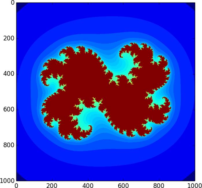
Figure 12-1. Julia set used for parallel computation
Performance-wise, it takes about 1.4 seconds to compute this Julia set on a domain with a resolution of 1,000 × 1,000 points.
Using prange
Upon inspection, it is clear that the escape computation does not depend on any previous loop iteration. This makes our loop an ideal candidate for parallelization, because each loop iteration is independent of all others.
As mentioned earlier, we first need to cimport prange from cython.parallel:
from cython.parallel cimport prange
Using prange is simple, provided we have already taken the necessary steps to ensure no Python objects are used inside the loop body. First we place the loop inside a with nogil block, and convert our outer loop’s range call to prange:
def calc_julia(...):
# ...
with nogil:
for i inprange(resolution + 1):
real = -bound + i * step
for j inrange(resolution + 1):
# ...
# ...
This pattern is so common that prange has a nogil keyword argument that is equivalent to the preceding example:
def calc_julia(...):
# ...
for i inprange(resolution + 1, nogil=True):
real = -bound + i * step
for j inrange(resolution + 1):
# ...
Once we use prange, we must ensure that we compile with OpenMP enabled. The standard compilation and linking flag to give compilers like gcc is -fopenmp. We can add a compiler directive comment at the top of julia.pyx:
# distutils: extra_compile_args = -fopenmp
# distutils: extra_link_args = -fopenmp
When rerunning the distutils script from the command line, ensure that the -fopenmp flag is included in the compilation and linking commands:
$ python setup_julia.py build_ext -i
Compiling julia.pyx because it changed.
Cythonizing julia.pyx
running build_ext
building 'julia' extension
gcc -fno-strict-aliasing -fno-common -dynamic -g -O2
-DNDEBUG -g -fwrapv -O3 -Wall -Wstrict-prototypes
-I[...] -c julia.c -o [...]/julia.o -fopenmp
gcc -bundle -undefined dynamic_lookup
[...]/julia.o -o [...]/julia.so -fopenmp
After taking these steps, we can run our test script as before, but this time the compiler enables threads when running the nested for loops, using all CPUs on our system to speed up execution. When we use this version of calc_julia and enable OpenMP, the runtime on an eight-core system improves to about 0.47 seconds, or a factor of three faster than the serial version. Not bad for a small amount of setup and an entirely trivial change to the source code. But we can do better: there are reasons why we are not utilizing more of the parallelism at our disposal.
prange Options
When prange is used with default parameters, it divides the loop range into equal-sized contiguous chunks, giving one chunk to each available thread. This strategy is bad for computing a Julia set: all points in red in Figure 12-1 (the fractal-like shape at the center for anyone reading in black and white) are in the set and maximize the number of loop iterations inside escape. The blue points (the outer area surrounding the fractal shape) are not in the set and require many fewer iterations. The unlucky threads assigned to the middle region get a chunk of the complex plane that contains many Julia set points, so these threads do the bulk of the work. What we want is to partition the work more evenly, or, in prange (and OpenMP) parlance, use a different chunksize, and possibly a different schedule.
Let’s try using a static schedule with prange and give it a chunksize of 1. This assigns rows of the counts array to threads in a round-robin, or cyclic, fashion:
def calc_julia(...):
# ...
for i inprange(resolution + 1, nogil=True,
schedule='static', chunksize=1):
# ...
With this modification, our runtime decreases to 0.26 seconds, about 5.5 times faster than the range-only version. Again, a nice payoff for a trivial change.
As indicated in the following list, there are other schedules besides static. Their behaviors allow control over different aspects of the threaded computation. The options are:
static
Iterations are assigned to threads in a fixed way at compile time. If chunksize is not given, the iterations are distributed in num_threads contiguous blocks, one block per thread. If chunksize is given, each chunk is assigned to threads in a round-robin fashion. This is best when the work is evenly distributed and generally known ahead of time.
dynamic
Threads ask the scheduler for the next chunk dynamically at runtime. The chunksize defaults to 1. A dynamic schedule is best when the workload is unevenly distributed and unknown ahead of time.
guided
Chunks are distributed dynamically, like with dynamic. Unlike with dynamic, the chunksize is not fixed but rather is proportional to the remaining iterations divided by the number of threads.
runtime
The schedule and chunksize are determined by either the openmp.openmp_set_schedule function or the OMP_SCHEDULE environment variable at runtime. This allows exploration of different schedules and chunksizes without recompiling, but may have poorer performance overall as no compile-time optimizations are possible.
TIP
Controlling the schedule and chunksize allows easy exploration of different parallel execution strategies and workload assignments. Typically static with a tuned chunksize is a good first approach; dynamic and guided incur runtime overhead and are appropriate in dynamically changing execution contexts. The runtime schedule provides maximum flexibility among all other schedule types.
We can use prange with start, stop, and step arguments, like range. In addition to the nogil, schedule, and chunksize optional arguments, prange also accepts a num_threads argument to control the number of threads to use during execution. If num_threads is not provided,prange uses as many threads as there are CPU cores available.
A performance boost of 5.5 for minor modifications to our Cython code is a nice result. This performance boost is multiplicative with the performance enhancements Cython already provides over pure Python.
Using prange for Reductions
Often we want to loop over an array and compute a scalar sum or product of values. For instance, suppose we want to compute the area fraction of our complex domain that is inside a Julia set. We can approximate this fraction by summing the number of points in the counts array that equaln_max and dividing by the total number of points. This gives us an opportunity to see how prange can speed up reduction operations, too.
Let’s call our function julia_fraction. It takes a typed memoryview for the counts array and a maxval argument, by default equal to n_max:
@boundscheck(False)
@wraparound(False)
def julia_fraction(int[:,::1] counts, int maxval=1000):
# ...
Our julia_fraction function needs to count up the number of n_max elements of our set, which we store in the total variable. We need the usual loop indexing variables as well:
def julia_fraction(...):
cdef:
int total = 0
int i, j, N, M
N = counts.shape[0]; M = counts.shape[1]
# ...
The core of our computation is, again, nested for loops. Once we compute the cardinality, we return it divided by the size of the counts array:
def julia_fraction(...):
# ...
for i inrange(N):
for j inrange(M):
if counts[i,j] == maxval:
total += 1
return total / float(counts.size)
When running this serial version of julia_fraction for a Julia set with c = 0.322 + 0.05j, we get an area fraction of about 0.24. Because we normalize by the total number of points in the complex domain, this fraction is independent of resolution. For a complex plane with a resolution of 4,000 × 4,000 points, it requires about 14 milliseconds to run.
Let’s substitute prange for range in the outer loop:
def julia_fraction(...):
# ...
for i inprange(N, nogil=True):
# ...
return total / float(counts.size)
With this trivial modification, runtime decreases to about 4 ms, an improvement of about a factor of 3.5. We can play with the schedule and chunksize as before, but they do not measurably affect performance. This may be related to the fact that this computation is likely memory bound and not CPU bound, so we cannot expect perfect speedup.
The generated code for this example uses OpenMP’s reduction features to parallelize the in-place addition. Because addition is commutative (i.e., the result is the same regardless of the order of the arguments), additive reductions can be automatically parallelized. Cython (via OpenMP) generates threaded code such that each thread computes the sum for a subset of the loop indices, and then all threads combine their individual sums into the resulting total. The nice part is that we just have to change range to prange to see the performance boost.
For the record, the equivalent NumPy operation is:
frac = np.sum(counts == maxval) / float(counts.size)
It yields an identical result but takes approximately nine times longer to compute than the prange version.
Interestingly, if we nudge the c value to 0.326 + 0.05j, the area fraction drops to 0.0. This is consistent with the Julia set for this value of c, which is disconnected and nowhere dense.
Parallel Programming Pointers and Pitfalls
Cython’s prange is easy to use, but as we see when computing the area fraction, prange provides a speedup of only 3.5, which is noticeably less than the speedup of 5.5 when we use prange to compute the corresponding Julia set. This boost is still far from perfect scaling on an eight-core system. We are glad for the extra performance boost, but in general it is very difficult to achieve perfect scaling, even when we have an embarrassingly parallel CPU-bound computation. This is true independent of using Cython: achieving ideal parallel scaling is just plain hard.
To better illustrate why perfect utilization is often elusive, consider a typical stencil operation like a five-point nearest-neighbor averaging filter on a two-dimensional C-contiguous array. The core computation is conceptually straightforward—for a given row and column index, add up the array elements nearby and assign the average to an output array:
def filter(...):
# ...
for i inrange(nrows):
for j inrange(ncols):
b[i,j] = (a[i,j] + a[i-1,j] + a[i+1,j] +
a[i,j-1] + a[i,j+1]) / 5.0
We can replace the outer range with prange, as we did with the Julia set computations. But for this straightforward implementation, performance is worse, not better, with prange. Part of the reason is that the loop body primarily accesses noncontiguous array elements. Because of the lack of locality, the CPU’s cache cannot be as effective. Besides nonlocality, there are other factors at play that conspire to slow down prange or any other naive thread-based implementation of the preceding loop.
There are some rules of thumb for using prange:
§ prange works well with embarrassingly parallel CPU-bound operations.
§ Memory-bound operations with many nonlocal reads and writes can be challenging to speed up.
§ It is easier to achieve linear speedup with fewer threads.
§ Using an optimized thread-parallel library is often the best way to use all cores for common operations.
With these warnings in mind, it is nevertheless useful to have prange at our disposal, especially given its ease of use. So long as our loop body does not interact with Python objects, using prange is nearly trivial.
Summary
Cython allows us to circumvent CPython’s global interpreter lock, so long as we cleanly separate our Python-interacting code from our Python-independent code. After doing so, we can easily access thread-based parallelism via Cython’s built-in prange.
We saw in this chapter how prange can provide extra performance boosts for loop-centric operations, and how prange provides control over how work is assigned to threads. Thread-based parallelism in other languages is error prone and can be very challenging to get right. Cython’sprange makes it straightforward and comparatively easy to enable threads for many performance bottlenecks.
[22] To follow along with the examples in this chapter, please see https://github.com/cythonbook/examples.
All materials on the site are licensed Creative Commons Attribution-Sharealike 3.0 Unported CC BY-SA 3.0 & GNU Free Documentation License (GFDL)
If you are the copyright holder of any material contained on our site and intend to remove it, please contact our site administrator for approval.
© 2016-2025 All site design rights belong to S.Y.A.