Functional Python Programming (2015)

Chapter 14. The PyMonad Library

A monad allows us to impose an order on expression evaluation in an otherwise lenient language. We can use a monad to insist that an expression such as a + b + c is evaluated in left-to-right order. Generally, there seems to be no point to a monad. When we want files to have their content read or written in a specific order, however, a monad is a handy way to assure that the read() and write() functions are evaluated in a particular order.

Languages that are lenient and have optimizing compilers benefit from monads to impose order on evaluation of expressions. Python, for the most part, is strict and does not optimize. We have little practical use for monads.

However, the PyMonad module is more than just monads. There are a number of functional programming features that have a distinctive implementation. In some cases, the PyMonad module can lead to programs which are more succinct and expressive than those written using only the standard library modules.

Downloading and installing

The PyMonad module is available on Python Package Index (PyPi). In order to add PyMonad to your environment, you'll need to use pip or Easy Install. Here are some typical situations:

· If you have Python 3.4 or higher, you have both of these installation package tools

· If you have Python 3.x, you may already have either one of the necessary installers because you've added packages already

· If you have Python 2.x, you should consider an upgrade to Python 3.4

· If you don't have pip or Easy Install, you'll need to install them first; consider upgrading to Python 3.4 to get these installation tools

Visit https://pypi.python.org/pypi/PyMonad/ for more information.

For Mac OS and Linux developers, the command pip install PyMonad or easy_install-3.3 pymonad must be run using the sudo command. When running a command such as sudo easy_install-3.3 pymonad, you'll be prompted for your password to assure that you have the administrative permissions necessary to do the installation. For Windows developers, the sudo command is not relevant, but you do need to have administrative rights.

Once the pymonad package is installed, you can confirm it using the following commands:

>>> import pymonad

>>> help(pymonad)

This will display the docstring module and confirm that things really are properly installed.

Functional composition and currying

Some functional languages work by transforming a multiargument function syntax into a collection of single argument functions. This process is called currying—it's named after logician Haskell Curry, who developed the theory from earlier concepts.

Currying is a technique for transforming a multiargument function into higher order single argument functions. In the simple case, we have a function ; given two arguments x and y, this will return some resulting value, z. We can curry this into two functions: and . Given the first argument value, x, the function returns a new one-argument function, returns a new one-argument function, . This second function can be given an argument, y, and will return the resulting value, z.

We can evaluate a curried function in Python as follows: f_c(2)(3). We apply the curried function to the first argument value of 2, creating a new function. Then, we apply that new function to the second argument value of 3.

This applies recursively to functions of any complexity. If we start with a function , we curry this into a function . This is done recursively. First, the function returns a new function with the b and c arguments, . Then we can curry the returned two-argument function to create .

We can evaluate this curried function with g_c(1)(2)(3). When we apply to an argument of 1, we get a function; when we apply this returned function to 2, we get another function. When we apply the final function to 3, we get the expected result. Clearly, formal syntax is bulky, so we use some syntactic sugar to reduce g_c(1)(2)(3) to something more palatable like g(1,2,3).

Let's look at a concrete example in Python, for example, we have a function like the following one:

from pymonad import curry

@curry

def systolic_bp(bmi, age, gender_male, treatment):

return 68.15+0.58*bmi+0.65*age+0.94*gender_male+6.44*treatment

This is a simple, multiple-regression-based model for systolic blood pressure. This predicts blood pressure from body mass index (BMI), age, gender (1 means male), and history of previous treatment (1 means previously treated). For more information on the model and how it's derived, visit http://sphweb.bumc.bu.edu/otlt/MPH-Modules/BS/BS704_Multivariable/BS704_Multivariable7.html.

We can use the systolic_bp() function with all four arguments, as follows:

>>> systolic_bp(25, 50, 1, 0)

116.09

>>> systolic_bp(25, 50, 0, 1)

121.59

A male person with a BMI of 25, age 50, and no previous treatment will likely have a blood pressure of 116. The second example shows a similar woman with a history of treatment who will likely have a blood pressure of 121.

Because we've used the @curry decorator, we can create intermediate results that are similar to partially applied functions. Take a look at the following command snippet:

>>> treated= systolic_bp(25, 50, 0)

>>> treated(0)

115.15

>>> treated(1)

121.59

In the preceding case, we evaluated the systolic_bp(25, 50, 0) method to create a curried function and assigned this to the variable treatment. The BMI, age, and gender values don't typically change for a given patient. We can now apply the new function,treatment, to the remaining argument to get different blood pressure expectations based on patient history.

This is similar in some respects to the functools.partial() function. The important difference is that currying creates a function that can work in a variety of ways. The functools.partial() function creates a more specialized function that can only be used with the given set of bound values.

Here's an example of creating some additional curried functions:

>>> g_t= systolic_bp(25, 50)

>>> g_t(1, 0)

116.09

>>> g_t(0, 1)

121.59

This is a gender-based treatment function based on our initial model. We must provide gender and treatment values to get a final value from the model.

Using curried higher-order functions

While currying is simple to visualize using ordinary functions, the real value shows up when we apply currying to higher-order functions. In the ideal situation, the functools.reduce() function would be "curryable" so that we can do this:

sum= reduce(operator.add)

prod= reduce(operator.mul)

The reduce() function, however, isn't curryable by the pymonad library, so this doesn't actually work. If we define our own reduce() function, however, we can then curry it as shown previously. Here's an example of a home-brewed reduce() function that can be used as shown earlier:

import collections.abc

from pymonad import curry

@curry

def myreduce(function, iterable_or_sequence):

if isinstance(iterable_or_sequence, collections.abc.Sequence):

iterator= iter(iterable_or_sequence)

else:

iterator= iterable_or_sequence

s = next(iterator)

for v in iterator:

s = function(s,v)

return s

The myreduce() function will behave like the built-in reduce() function. The myreduce() function works with an iterable or a sequence object. Given a sequence, we'll create an iterator; given an iterable object, we'll simply use it. We initialize the result with the first item in the iterator. We apply the function to the ongoing sum (or product) and each subsequent item.

Note

It's also possible to wrap the built-in reduce() function to create a curryable version. That's only two lines of code; an exercise left for you.

Since the myreduce() function is a curried function, we can now use it to create functions based on our higher-order function, myreduce():

>>> from operator import *

>>> sum= myreduce(add)

>>> sum([1,2,3])

6

>>> max= myreduce(lambda x,y: x if x > y else y)

>>> max([2,5,3])

5

We defined our own version of the sum() function using the curried reduce applied to the add operator. We also defined our own version of the default max() function using a lambda object that picks the larger of two values.

We can't easily create the more general form of the max() function this way, because currying is focused on positional parameters. Trying to use the key= keyword parameter adds too much complexity to make the technique work toward our overall goals of succinct and expressive functional programs.

To create a more generalized version of the max() function, we need to step outside the key= keyword parameter paradigm that functions such as max(), min(), and sorted() rely on. We would have to accept the higher-order function as the first argument in the same way as filter(), map(), and reduce() functions do. We could also create our own library of more consistent higher-order curried functions. These functions would rely exclusively on positional parameters. The higher-order function would be provided first so that our own curried max(function, iterable) method would follow the pattern set by the map(), filter(), and functools.reduce() functions.

Currying the hard way

We can create curried functions manually, without using the decorator from the pymonad library; one way of doing this is to execute the following commands:

def f(x, *args):

def f1(y, *args):

def f2(z):

return (x+y)*z

if args:

return f2(*args)

return f2

if args:

return f1(*args)

return f1

This curries a function, , into a function, f(x), which returns a function. Conceptually, . We then curried the intermediate function to create the f1(y) and f2(z) function.

When we evaluate the f(x) function, we'll get a new function, f1, as a result. If additional arguments are provided, those arguments are passed to the f1 function for evaluation, either resulting in a final value or another function.

Clearly, this is potentially error-prone. It does, however, serve to define what currying really means and how it's implemented in Python.

Functional composition and the PyMonad multiplication operator

One of the significant values of curried functions is the ability to combine them via functional composition. We looked at functional composition in Chapter 5, Higher-order Functions, and Chapter 11, Decorator Design Techniques.

When we've created a curried function, we can easily perform function composition to create a new, more complex curried function. In this case, the PyMonad package defines the * operator for composing two functions. To show how this works, we'll define two curried functions that we can compose. First, we'll define a function that computes the product, and then we'll define a function that computes a specialized range of values.

Here's our first function that computes the product:

import operator

prod = myreduce(operator.mul)

This is based on our curried myreduce() function that was defined previously. It uses the operator.mul() function to compute a "times-reduction" of an iterable: we can call a product a times-reduce of a sequence.

Here's our second curried function that will produce a range of values:

@curry

def alt_range(n):

if n == 0: return range(1,2) # Only 1

if n % 2 == 0:

return range(2,n+1,2)

else:

return range(1,n+1,2)

The result of the alt_range() function will be even values or odd values. It will have only values up to (and including) n, if n is odd. If n is even, it will have only even values up to n. The sequences are important for implementing the semifactorial or double factorial function, .

Here's how we can combine the prod() and alt_range() functions into a new curried function:

>>> semi_fact= prod * alt_range

>>> semi_fact(9)

945

The PyMonad * operator here combines two functions into a composite function, named semi_fact. The alt_range() function is applied to the arguments. Then, the prod() function is applied to the results of the alt_range function.

By doing this manually in Python, we're effectively creating a new lambda object:

semi_fact= lambda x: prod(alt_range(x))

The composition of curried functions involves somewhat less syntax than creating a new lambda object.

Ideally, we would like to use functional composition and curried functions like this:

sumwhile= sum * takewhile(lambda x: x > 1E-7)

This will define a version of the sum() function that works with infinite sequences, stopping the generation of values when the threshold had been met. This doesn't seem to work because the pymonad library doesn't seem to handle infinite iterables as well as it handles the internal List objects.

Functors and applicative functors

The idea of a functor is a functional representation of a piece of simple data. A functor version of the number 3.14 is a function of zero arguments that returns this value. Consider the following example:

pi= lambda : 3.14

We created a zero-argument lambda object that has a simple value.

When we apply a curried function to a functor, we're creating a new curried functor. This generalizes the idea of "apply a function to an argument to get value" by using functions to represent the arguments, the values, and the functions themselves.

Once everything in our program is a function, then all processing is simply a variation on the theme of functional composition. The arguments and results of curried functions can be functors. At some point, we'll apply a getValue() method to a functor object to get a Python-friendly, simple type that we can use in uncurried code.

Since all we've done is functional composition, no calculation needs to be done until we actually demand a value using the getValue() method. Instead of performing a lot of calculations, our program defines a complex object that can produce a value when requested. In principle, this composition can be optimized by a clever compiler or runtime system.

When we apply a function to a functor object, we're going to use a method similar to map() that is implemented as the * operator. We can think of the function * functor or map(function, functor) methods as a way to understand the role a functor plays in an expression.

In order to work politely with functions that have multiple arguments, we'll use the & operator to build composite functors. We'll often see functor & functor method to build a functor object from a pair of functors.

We can wrap Python simple types with a subclass of the Maybe functor. The Maybe functor is interesting, because it gives us a way to deal gracefully with missing data. The approach we used in Chapter 11, Decorator Design Techniques, was to decorate built-in functions to make them None aware. The approach taken by the PyMonad library is to decorate the data so that it gracefully declines being operated on.

There are two subclasses of the Maybe functor:

· Nothing

· Just(some simple value)

We use Nothing as a stand-in for the simple Python value of None. This is how we represent missing data. We use Just(some simple value) to wrap all other Python objects. These functors are function-like representations of constant values.

We can use a curried function with these Maybe objects to tolerate missing data gracefully. Here's a short example:

>>> x1= systolic_bp * Just(25) & Just(50) & Just(1) & Just(0)

>>> x1.getValue()

116.09

>>> x2= systolic_bp * Just(25) & Just(50) & Just(1) & Nothing

>>> x2.getValue() is None

True

The * operator is functional composition: we're composing the systolic_bp() function with an argument composite. The & operator builds a composite functor that can be passed as an argument to a curried function of multiple arguments.

This shows us that we get an answer instead of a TypeError exception. This can be very handy when working with large, complex datasets in which data could be missing or invalid. It's much nicer than having to decorate all of our functions to make them None aware.

This works nicely for curried functions. We can't operate on the Maybe functors in uncurried Python code as functors have very few methods.

Note

We must use the getValue() method to extract the simple Python value for uncurried Python code.

Using the lazy List() functor

The List() functor can be confusing at first. It's extremely lazy, unlike Python's built-in list type. When we evaluate the built-in list(range(10)) method, the list() function will evaluate the range() object to create a list with 10 items. The PyMonad List() functor, however, is too lazy to even do this evaluation.

Here's the comparison:

>>> list(range(10))

[0, 1, 2, 3, 4, 5, 6, 7, 8, 9]

>>> List(range(10))

[range(0, 10)]

The List() functor did not evaluate the range() object, it just preserved it without being evaluated. The PyMonad.List() function is useful to collect functions without evaluating them. We can evaluate them later as required:

>>> x= List(range(10))

>>> x

[range(0, 10)]

>>> list(x[0])

[0, 1, 2, 3, 4, 5, 6, 7, 8, 9]

We created a lazy List object with a range() object. Then we extracted and evaluated a range() object at position 0 in that list.

A List object won't evaluate a generator function or range() object; it treats any iterable argument as a single iterator object. We can, however, use the * operator to expand the values of a generator or the range() object.

Note

Note that there are several meanings for * operator: it is the built-in mathematical times operator, the function composition operator defined by PyMonad, and the built-in modifier used when calling a function to bind a single sequence object as all of the positional parameters of a function. We're going to use the third meaning of the * operator to assign a sequence to multiple positional parameters.

Here's a curried version of the range() function. This has a lower bound of 1 instead of 0. It's handy for some mathematical work because it allows us to avoid the complexity of the positional arguments in the built-in range() function.

@curry

def range1n(n):

if n == 0: return range(1,2) # Only 1

return range(1,n+1)

We simply wrapped the built-in range() function to make it curryable by the PyMonad package.

Since a List object is a functor, we can map functions to the List object. The function is applied to each item in the List object. Here's an example:

>>> fact= prod * range1n

>>> seq1 = List(*range(20))

>>> f1 = fact * seq1

>>> f1[:10]

[1, 1, 2, 6, 24, 120, 720, 5040, 40320, 362880]

We defined a composite function, fact(), which was built from the prod() and range1n() functions shown previously. This is the factorial function, . We created a List() functor, seq1, which is a sequence of 20 values. We mapped the fact() function to the seq1functor, which created a sequence of factorial values, f1. We showed the first 10 of these values earlier.

Note

There is a similarity between the composition of functions and the composition of a function and a functor. Both prod*range1n and fact*seq1 use functional composition: one combines things that are obviously functions, and the other combines a function and a functor.

Here's another little function that we'll use to extend this example:

@curry

def n21(n):

return 2*n+1

This little n21() function does a simple computation. It's curried, however, so we can apply it to a functor like a List() function. Here's the next part of the preceding example:

>>> semi_fact= prod * alt_range

>>> f2 = semi_fact * n21 * seq1

>>> f2[:10]

[1, 3, 15, 105, 945, 10395, 135135, 2027025, 34459425, 654729075]

We've defined a composite function from the prod() and alt_range() functions shown previously. The function f2 is semifactorial or double factorial, . The value of the function f2 is built by mapping our small n21() function applied to the seq1 sequence. This creates a new sequence. We then applied the semi_fact function to this new sequence to create a sequence of values that parallels the sequence of values.

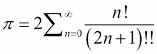
We can now map the / operator to the map() and operator.truediv parallel functors:

>>> 2*sum(map(operator.truediv, f1, f2))

3.1415919276751456

The map() function will apply the given operator to both functors, yielding a sequence of fractions that we can add.

Note

The f1 & f2 method will create all combinations of values from the two List objects. This is an important feature of List objects: they readily enumerate all combinations allowing a simple algorithm to compute all alternatives and filter the alternatives for the proper subset. This is something we don't want; that's why we used the map() function instead of the operator.truediv * f1 & f2 method.

We defined a fairly complex calculation using a few functional composition techniques and a functor class definition. Here's the full definition for this calculation:

Ideally, we prefer not to use a fixed sized List object. We'd prefer to have a lazy and potentially infinite sequence of integer values. We could then use a curried version of sum() and takewhile() functions to find the sum of values in the sequence until the values are too small to contribute to the result. This would require an even lazier version of the List() object that could work with the itertools.counter() function. We don't have this potentially infinite list in PyMonad 1.3; we're limited to a fixed sized List() object.

Monad concepts, the bind() function and the Binary Right Shift operator

The name of the PyMonad library comes from the functional programming concept of a monad, a function that has a strict order. The underlying assumption behind much functional programming is that functional evaluation is liberal: it can be optimized or rearranged as necessary. A monad provides an exception that imposes a strict left-to-right ordering.

Python, as we have seen, is strict. It doesn't require monads. We can, however, still apply the concept in places where it can help clarify a complex algorithm.

The technology for imposing strict evaluation is a binding between a monad and a function that will return a monad. A flat expression will become nested bindings that can't be reordered by an optimizing compiler. The bind() function is mapped to the >> operator, allowing us to write expressions like this:

Just(some file) >> read header >> read next >> read next

The preceding expression would be converted to the following:

bind(bind(bind(Just(some file), read header), read next), read next)

The bind() functions assure that a strict left-to-right evaluation is imposed on this expression when it's evaluated. Also, note that the preceding expression is an example of functional composition. When we create a monad with the >> operator, we're creating a complex object that will be evaluated when we finally use the getValue() method.

The Just() subclass is required to create a simple monad compatible object that wraps a simple Python object.

The monad concept is central to expressing a strict evaluation order—in a language that's heavily optimized and lenient. Python doesn't require a monad because it uses left-to-right strict evaluation. This makes the monad difficult to demonstrate because it doesn't really do something completely novel in a Python context. Indeed, the monad redundantly states the typical strict rules that Python follows.

In other languages, such as Haskell, a monad is crucial for file input and output where strict ordering is required. Python's imperative mode is much like a Haskell do block, which has an implicit Haskell >>= operator to force the statements to be evaluated in order. (PyMonad uses the bind() function and the >> operator for Haskell's >>= operation.)

Implementing simulation with monads

Monads are expected to pass through a kind of "pipeline": a monad will be passed as an argument to a function and a similar monad will be returned as the value of the function. The functions must be designed to accept and return similar structures.

We'll look at a simple pipeline that can be used for simulation of a process. This kind of simulation may be a formal part of some Monte Carlo simulation. We'll take the Monte Carlo simulation literally and simulate a casino dice game, Craps. This involves what might be thought of as stateful rules for a fairly complex simulation.

There's a lot of very strange gambling terminology involved. We can't provide much background about the various buzzwords involved. In some cases, the origins are lost in history.

Craps involves someone rolling the dice (a shooter) and additional bettors. The game works like this:

The first roll is called a come out roll. There are three conditions:

1. If the dice total is 7 or 11, the shooter wins. Anyone betting on the pass line will be paid off as a winner, and all other bets lose. The game is over, and the shooter can play again.

2. If the dice total is 2, 3, or 12, the shooter loses. Anyone betting on the don't pass line will win, and all other bets lose. The game is over, and the shooter must pass the dice to another shooter.

3. Any other total (that is, 4, 5, 6, 8, 9, or 10) establishes a point. The game changes state from the come out roll to the point roll. The game continues.

If a point was established, each point roll is evaluated with three conditions:

· If the dice total is 7, the shooter loses. Indeed, almost all bets are losers except for don't pass bets and a special proposition bet. Since the shooter lost, the dice are passed to another shooter.

· If the dice totals the original point, the shooter wins. Anyone betting on the pass line will be paid off as a winner, and all other bets lose. The game is over, and the shooter can play again.

· Any other total continues the game with no resolution.

The rules involve a kind of state change. We can look at this as a sequence of operations rather than a state change. There's one function that must be used first. Another recursive function is used after that. In this way, it fits the monad design pattern nicely.

As a practical matter, a casino allows numerous fairly complex side bets during the game. We can evaluate those separately from the essential rules of the game. Many of those bets (the propositions, field bets, and buying a number) are bets a player simply makes during the point roll phase of the game. There's an additional come and don't come pair of bets that establishes a point-within-a-point nested game. We'll stick the the basic outline of the game for the following example.

We'll need a source of random numbers:

import random

def rng():

return (random.randint(1,6), random.randint(1,6))

The preceding function will generate a pair of dice for us.

Here's our expectation from the overall game:

def craps():

outcome= Just(("",0, []) ) >> come_out_roll(rng) >> point_roll(rng)

print(outcome.getValue())

We create an initial monad, Just(("",0, [])), to define the essential type we're going to work with. A game will produce a three tuple with an outcome, a point, and a sequence of rolls. Initially, it's a default three tuple to define the type we're working with.

We pass this monad to two other functions. This will create a resulting monad, outcome, with the results of the game. We used the >> operator to connect the functions in the specific order they must be executed. In an optimizing language, this will prevent the expression from being rearranged.

We get the value of the monad at the end using the getValue() method. Since the monad objects are lazy, this request is what triggers the evaluation of the various monads to create the required output.

The come_out_roll() function has the rng() function curried as the first argument. The monad will become the second argument to this function. The come_out_roll() function can roll the dice and apply the come out rules to determine if we have a win, a loss, or a point.

The point_roll() function also has the rng() function curried as the first argument. The monad will become the second argument. The point_roll() function can then roll the dice to see if the bet is resolved. If the bet is unresolved, this function will operate recursively to continue looking for resolution.

The come_out_roll() function looks like this:

@curry

def come_out_roll(dice, status):

d= dice()

if sum(d) in (7, 11):

return Just(("win", sum(d), [d]))

elif sum(d) in (2, 3, 12):

return Just(("lose", sum(d), [d]))

else:

return Just(("point", sum(d), [d]))

We rolled the dice once to determine if we have a first-roll win, loss, or point. We return an appropriate monad value that includes the outcome, a point value, and the roll of the dice. The point values for an immediate win and immediate loss aren't really meaningful. We could sensibly return a 0 here, since no point was really established.

The point_roll() function looks like this:

@curry

def point_roll(dice, status):

prev, point, so_far = status

if prev != "point":

return Just(status)

d = dice()

if sum(d) == 7:

return Just(("craps", point, so_far+[d]))

elif sum(d) == point:

return Just(("win", point, so_far+[d]))

else:

return Just(("point", point, so_far+[d])) >> point_roll(dice)

We decomposed the status monad into the three individual values of the tuple. We could have used small lambda objects to extract the first, second, and third values. We could also have used the operator.itemgetter() function to extract the tuples' items. Instead, we used multiple assignment.

If a point was not established, the previous state will be "win" or "lose". The game was resolved in a single throw, and this function simply returns the status monad.

If a point was established, the dice are rolled and rules applied to the new roll. If roll is 7, the game is a loser and a final monad is returned. If the roll is the point, the game is a winner and the appropriate monad is returned. Otherwise, a slightly revised monad is passed to the point_roll() function. The revised status monad includes this roll in the history of rolls.

A typical output looks like this:

>>> craps()

('craps', 5, [(2, 3), (1, 3), (1, 5), (1, 6)])

The final monad has a string that shows the outcome. It has the point that was established and the sequence of dice rolls. Each outcome has a specific payout that we can use to determine the overall fluctuation in the bettor's stake.

We can use simulation to examine different betting strategies. We might be searching for a way to defeat any house edge built into the game.

Note

There's a small asymmetry in the basic rules of the game. Having 11 as an immediate winner is balanced by having 3 as an immediate loser. The fact that 2 and 12 are also losers is the basis of the house's edge of 5.5 percent (1/18 = 5.5) in this game. The idea is to determine which of the additional betting opportunities will dilute this edge.

A great deal of clever Monte Carlo simulation can be built with a few simple, functional programming design techniques. The monad, in particular, can help structure these kinds of calculations when there are complex orders or internal states.

Additional PyMonad features

One of the other features of PyMonad is the confusingly named monoid. This comes directly from mathematics and it refers to a group of data elements that have an operator, an identity element, and the group is closed with respect to that operator. When we think of natural numbers, the add operator, and an identity element 0, this is a proper monoid. For positive integers, with an operator *, and an identity value of 1, we also have a monoid; strings using | as an operator and an empty string as an identity element also qualifies.

PyMonad includes a number of predefined monoid classes. We can extend this to add our own monoid class. The intent is to limit a compiler to certain kinds of optimizations. We can also use the monoid class to create data structures which accumulate a complex value, perhaps including a history of previous operations.

Much of this provides insight into functional programming. To paraphrase the documentation, this is an easy way to learn about functional programming in, perhaps, a slightly more forgiving environment. Rather than learning an entire language and toolset to compile and run functional programs, we can just experiment with interactive Python.

Pragmatically, we don't need too many of these features because Python is already stateful and offers strict evaluation of expressions. There's no practical reason to introduce stateful objects in Python, or strictly-ordered evaluation. We can write useful programs in Python by mixing functional concepts with Python's imperative implementation. For that reason, we won't delve any more deeply into PyMonad.

Summary

In this chapter, we looked at how we can use the PyMonad library to express some functional programming concepts directly in Python. The module shows many important functional programming techniques.

We looked at the idea of currying, a function that allows combinations of arguments to be applied to create new functions. Currying a function also allows us to use functional composition to create more complex functions from simpler pieces. We looked at functors that wrap simple data objects to make them into functions which can also be used with functional composition.

Monads are a way to impose a strict evaluation order when working with an optimizing compiler and lazy evaluation rules. In Python, we don't have a good use case for monads, because Python is an imperative programming language under the hood. In some cases, imperative Python may be more expressive and succinct than a monad construction.

In the next chapter, we'll look at how we can apply functional programming techniques to build web services applications. The idea of HTTP could be summarized as response = httpd(request). Ideally, HTTP is stateless, making it a perfect match for functional design. However, most web sites will maintain state, using cookies to track session state.