Beginning Python Games Development With Pygame (2015)

CHAPTER 9

Exploring the Third Dimension

You’ve seen how to take a point in three-dimensional space and project it onto the screen so that it can be rendered. Projection is only part of the process of rendering a 3D scene; you also need to manipulate the points in the game to update the scene from frame to frame. This chapter introduces the matrix, which is a kind of mathematical shortcut used to manipulate the position and orientation of objects in a game.

You will also learn how to use Pygame with OpenGL to access the 3D graphics capabilities of your graphics card to create impressive visuals, on par with commercial games.

What Is a Matrix?

Long before that movie, mathematicians and game programmers were using matrices. A matrix is a grid of numbers that can be any size, but in 3D graphics the most useful matrix is the 4 × 4 matrix. This section covers how to use matrices to position objects in a 3D world.

It takes a few different pieces of information to describe how a 3D object will look in a game, but its basic shape is defined by a collection of points. In the previous chapter we created a model of cube by building a list of points along its edges. More typically the list of points for a game model is read from a file created with specialized software. However the model is created, it has to be placed at a location in the game world, pointing in an appropriate direction and possibly scaled to a new size. These transformations of the points in a 3D model are done with matrices.

Understanding how matrices work would require a lot of math that is beyond the scope of this book. Fortunately you don’t need to know how they work to be able to use them. It is more important to understand what matrices do, and how they relate to the 3D graphics on screen. This is something that is generally not covered well in textbooks, and is probably why matrices have a reputation for being a little mysterious. Let’s take a look at a matrix and try to make sense of it. The following is one of the simplest types of matrix:

[ 1 0 0 0 ]
[ 0 1 0 0 ]
[ 0 0 1 0 ]
[ 0 0 0 1 ]

This matrix consists of 16 numbers arranged into four rows and four columns. For most matrices used in 3D graphics, only the first three columns will differ; the fourth column will consist of three zeros followed by a 1.

Note Matrices can contain any number of rows and columns, but when I use the word matrix in this book I am referring to the 4 × 4 matrix, commonly used in 3D graphics.

The first three rows represent an axis in 3D space, which is simply three vectors that point in the x, y, and z directions of the transformation. It helps to think of these three vectors as right, up, and forward to avoid confusion with the x, y, and z axes of the world. These vectors are always relative to the object being transformed. For example, if the game character was a humanoid male, then the matrix may be in the center of his chest somewhere. The right vector would point out from his right arm, the up vector would point out of the top of his head, and the forward vector would point forward through his chest.

The fourth row is the matrix translation, which is where the coordinate (0, 0, 0) would end up if it were transformed with this matrix. Because most 3D objects are modeled around the origin, you can think of the translation as the position of the object, once it has been transformed.

If we transformed a tank with this matrix, where would it end up? Well, the translation is (0, 0, 0) so it would be in the center of the screen. The right vector is (1, 0, 0), which would mean that the right side of the tank was facing in the direction of the x axis. The up vector is (0, 1, 0), which faces the top of the screen in the positive y direction. Finally, the forward vector is (0, 0, 1), which would place the turret of the tank pointing directly out of the screen. See Figure 9-1 for a breakdown of the parts of a matrix.

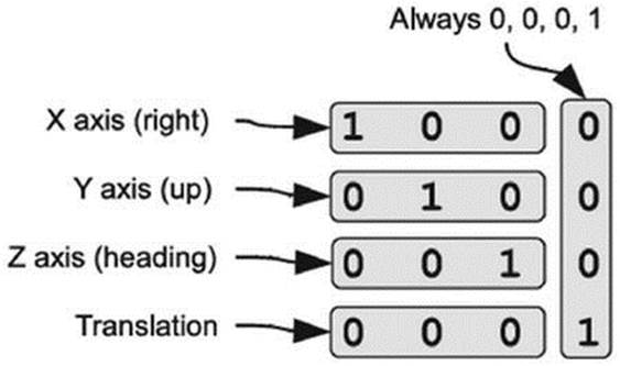
Figure 9-1. Components of a matrix

Note Some books display matrices with the rows and columns flipped, so that the translation part is in the right column rather than the bottom row. Game programmers typically use the same convention as this book because it can be more efficient to store matrices in memory this way.

Using the Matrix Class

The Game Objects library contains a class named Matrix44 that we can use with Pygame. Let’s experiment with it in the interactive interpreter. The following code shows how you would import Matrix44 and start using it:

>>> from gameobjects.matrix44 import *
>>> identity = Matrix44()
>>> print(identity)

The first line imports the Matrix44 class from the gameobjects.matrix44 module. The second line creates a Matrix44 object, which defaults to the identity matrix, and names it identity. The third line prints the value of identity to the console, which results in the following output:

[ 1 0 0 0 ]
[ 0 1 0 0 ]
[ 0 0 1 0 ]
[ 0 0 0 1 ]

Let’s see what happens if we use the identity matrix to transform a point. The following code creates a tuple (1.0, 2.0, 3.0) that we will use to represent a point (a Vector3 object would also work here). It then uses the transform function of the matrix object to transform the point and return the result as another tuple:

>>> p1 = (1.0, 2.0, 3.0)
>>> identity.transform(p1)

This produces the following output:

(1.0, 2.0, 3.0)

The point that was returned is the same as p1, which is what we would expect from the identity matrix. Other matrices have more interesting (and useful) effects, which we will cover in this chapter.

Matrix Components

It is possible to access the components of a matrix individually (see Figure 9-2). You can access individual values using the index operator ([]), which takes the row and column of the value in the matrix you are interested in. For example, matrix[3, 1] returns the value at row 3, column 1 and matrix[3, 1] = 2.0 would set that same value to 2.0. This value is actually the y component of the translation part of the matrix, so changing it would alter the height of an object over the ground.

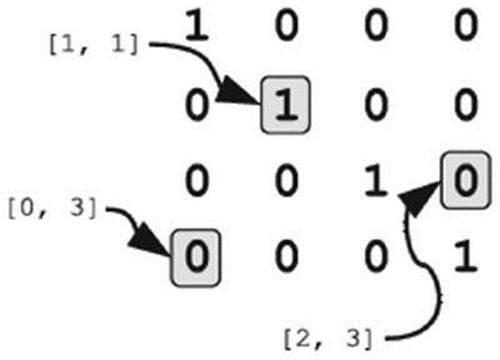
Figure 9-2. Matrix components

Individual rows of the matrix can be extracted by calling the get_row method, which returns the row as a tuple of four values. For example, matrix.get_row(0) returns row zero (top row, x axis), and matrix.get_row(3) returns the last row. There is also an equivalentset_row method, which takes the index of the row you want to set, and a sequence of up to four values to copy into the row. As with most methods of the Matrix44 class, get_row and set_row work with Vector3 objects as well as the built-in types.

The Matrix44 class also contains a number of attributes you can use to retrieve rows, which can be more intuitive than using the row index. For instance, rather than doing m.get_row(3) to retrieve the translation part of a matrix, you can use the attribute m.translate, which has the same effect. You can also replace m.set_row(3, (1, 2, 3)) with m.translate = (1, 2, 3)—both will set the first three values of row 3 to (1, 2, 3). Table 9-1 lists the attributes you can use to access rows in a matrix.

Table 9-1. Row Attributes for Matrix44 Objects

You can also get and set the columns of a matrix with get_column and set_column, which work in the same way as the row methods. They are perhaps less useful, because columns don’t give you as much relevant information as the rows do. One use for get_column is to check that the right column is (0, 0, 0, 1), because anything else may indicate an error in your code. Listing 9-1 is an example of how to check a matrix for validity. It uses Python’s assert keyword to check column 3 of the matrix. If the third column is (0, 0, 0, 1), then nothing happens; otherwise, Python will throw an AssertionError. You should never catch these types of exceptions; they are Python’s way of telling you that something is wrong with your code and that you should investigate the problem.

Tip Try to get into the habit of writing assert conditions. They are a good way of catching problems in your code early on. If you want Python to ignore assert statements in the code, invoke the script with python –O.

Listing 9-1. Checking Whether a Matrix Is Valid

from gameobjects.matrix44 import *

identity = Matrix44()
print(identity)
p1 = (1.0, 2.0, 3.0)
identity.transform(p1)

assert identity.get_column(3) == (0, 0, 0, 1), "Something is wrong with this matrix!"

Translation Matrix

A translation matrix is a matrix that adds a vector to the point being transformed. If we transform the points of a 3D model by a translation matrix, it will move the model so that its center is at a new coordinate in the world. You can create a translation matrix by callingMatrix44.translation, which takes the translation vector as three values. The following code creates and displays a translation matrix:

>>> p1 = (1.0, 2.0, 3.0)
>>> translation = Matrix44.translation(10, 5, 2)
>>> print(translation)
>>> translation.transform(p1)

This produces the following output:

[ 1 0 0 0 ]
[ 0 1 0 0 ]
[ 0 0 1 0 ]
[ 10 5 2 1 ]

The first three rows of a translation matrix are the same as the identity matrix; the translation vector is stored in the last row. When p1 is transformed, its components are added to the translation—in the same way as vector addition. Every object in a 3D game must be translated; otherwise, everything would be located in the center of the screen!

Manipulating the matrix translation is the primary way of moving a 3D object. You can treat the translation row of a matrix as the object’s coordinate and update it with time-based movement. Listing 9-2 is an example of how you might move a 3D model (in this case, a tank) forward, based on its current speed.

Listing 9-2. Example of Moving a 3D Object

tank_heading = Vector3(tank_matrix.forward)
tank_matrix.translation += tank_heading * tank_speed * time_passed

The first line in Listing 9-2 retrieves the tank’s heading. Assuming that the tank is moving in the same direction as it is pointing, its heading is the same as its forward vector (z axis). The second line calculates the distance the tank has moved since the previous frame by multiplying its heading by the tank’s speed and the time passed. The resulting vector is then added to the matrix translation. If this were done in every frame, the tank would move smoothly in the direction it is pointing.

Caution You can only treat the forward vector as a heading if the matrix has not been scaled (see the next section). If it has, then you must normalize the forward vector so that it has a length of one. If the tank in Listing 9-2 was scaled, you could calculate a forward heading withVector3(tank_matrix.forward).get_normalized().

Scale Matrix

A scale matrix is used to change the size of a 3D object, which can create useful effects in a game. For example, if you have a survival horror game with many zombies wandering about a desolate city, it might look a little odd if they were all exactly the same size. A little variation in height would make the hordes of undead look more convincing. Scale can also be varied over time to produce other visual effects; a crowd-pleasing fireball effect can be created by rapidly scaling a red sphere so that it engulfs an enemy and then slowly fades away.

The following code creates a scale matrix that would double the dimensions of an object. When we use it to transform p1, we get a point with components that are twice the original:

>>> scale = Matrix44.scale(2.0)
>>> print(scale)
>>> scale.transform(p1)

This produces the following output:

[ 2 0 0 0 ]
[ 0 2 0 0 ]
[ 0 0 2 0 ]
[ 0 0 0 1 ]

The scale value can also be less than one, which would make the model smaller. For example, Matrix44.scale(0.5) will create a matrix that makes a 3D object half the size.

Note If you create a scale matrix with a negative scale value, it will have the effect of flipping everything so that left becomes right, top becomes bottom, and front becomes back!

You can also create a scale matrix with three different values for each axis, which scales the object differently in each direction. For example, Matrix44.scale(2.0, 0.5, 3.0) will create a matrix that makes an object twice as wide, half as tall, and three times as deep! You are unlikely to need this very often, but it can be useful. For example, to simulate a plume of dust from a car tire, you could scale a model of a cloud of dust unevenly so that it looks like the tires are kicking it up.

To deduce the scale of a matrix, look at the axis vectors in the top-left 3 × 3 values. In an unscaled matrix, each vector of the axis has a length of one. For a scale matrix, the length (i.e., magnitude) of each vector is the scale for the corresponding axis. For example, the first axis vector in the scale matrix is (2, 0, 0), which has a length of two. The length may not be as obvious as this in all matrices, so this code demonstrates how to go about finding the scale of the x axis:

>>> x_axis_vector = Vector3(scale.x_axis)
>>> print(x_axis_vector.get_magnitude())

This produces the following result:

2.0

Rotation Matrix

Every object in a 3D game will have to be rotated at some point so that it faces in an appropriate direction. Most things face in the direction they are moving, but you can orient a 3D object in any direction you wish. Rotation is also a good way to draw attention to an object. For example,power-ups (ammo, extra lives, etc.) often rotate around the y axis so they stand out from the background scenery.

The simplest type of rotation matrix is a rotation about the x, y, or z axis, which you can create with the x_rotation, y_rotation, and z_rotation class methods in Matrix44 (see Figure 9-3).

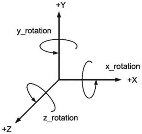
Figure 9-3. Rotation matrices

To predict which way a point will rotate, visualize yourself looking along the axis of rotation. Positive rotations go counterclockwise and negative rotations go clockwise. Let’s experiment with this in the interactive interpreter. We are going to rotate a point at (0, 10, 0), –45 degrees around the z axis (see Figure 9-4).

>>> z_rotate = Matrix44.z_rotation(radians(–45))
>>> print(z_rotate)
>>> a = (0, 10, 0)
>>> z_rotate.transform(a)

This displays a z rotation matrix, and the result of using it to translate the point (0, 10, 0):

[ 0.707107 -0.707107 0 0 ]
[ 0.707107 0.707107 0 0 ]
[ 0 0 1 0 ]
[ 0 0 0 1 ]

If the original point were the end of a watch hand at 12 o’clock, then the transformed point would be halfway between 1 and 2.

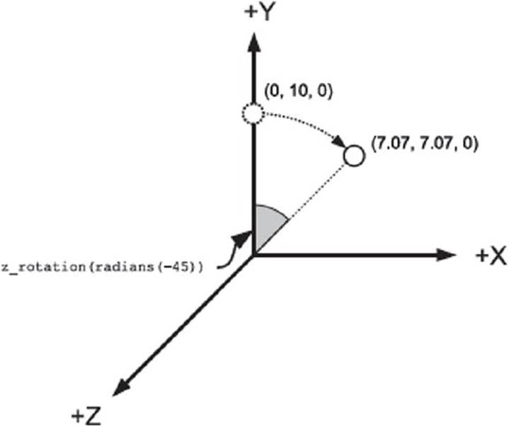
Figure 9-4. A rotation about the z axis

When working with 3D rotation, I find it helpful to visualize an axis for my head, where (0, 0, 0) is in my brain somewhere. The x axis points out of my right ear, the y axis points out the top of my head, and the z axis points out of my nose. If I were to rotate my head around the x axis, I would nod my head up and down. Rotating around the y axis would make me turn my head left or right. A rotation around the z axis would make me tilt my head quizzically from side to side. Alternatively, you can use your thumb and first two fingers to point along the positive direction of each axis and physically rotate your hand when you are thinking about rotations.

Matrix Multiplication

Often in a game you will need to do several transformations to a 3D object. For a tank game you would likely want to translate it to a position in the world and then rotate it to face the direction it is heading. You could transform the tank with both matrices, but it is possible to create a single matrix that has the combined effect by using matrix multiplication. When you multiply a matrix by another, you get a single matrix that does both transformations. Let’s test that by multiplying two translation matrices together:

>>> translate1 = Matrix44.translation(5, 10, 2)
>>> translate2 = Matrix44.translation(-7, 2, 4)
>>> print(translate1 * translate2)

This prints the result of multiplying translate1 with translate2:

[ 1 0 0 0 ]
[ 0 1 0 0 ]
[ 0 0 1 0 ]
[ –2 12 6 1 ]

The result is also a translation matrix. The last row (the translation part) in the matrix is (–2, 12, 6), which is the combined effect of translating by (5, 10, 2) and (–7, 2, 4). Matrices do not need to be of the same type to be multiplied together. Let’s try multiplying a rotation matrix by a translation matrix. The following code creates two matrices, translate and rotate, and a single matrix, translate_rotate, which has the effect of both:

>>> translate = Matrix44.translation(5, 10, 0)
>>> rotate = Matrix44.y_rotation(radians(45))
>>> translate_rotate = translate * rotate
>>> print(translate_rotate)

This displays the result of multiplying the two matrices:

[ 0.707107 0 -0.707107 0 ]
[ 0 1 0 0 ]
[ 0.707107 0 0.707107 0 ]
[ 5 10 0 1 ]

If we were to transform a tank with translate_rotate, it would place it at the coordinate (5, 10, 0), rotated 45 degrees around the y axis.

Although matrix multiplication is similar to multiplying numbers together, there is a significant difference: the order of multiplication matters. With numbers, the result of A*B is the same as B*A, but this would not be true if A and B were matrices. The translate_rotate matrix we produced first translates the object to (5, 10, 0), then rotates it around its center point. If we do the multiplication in the opposite order, the resulting matrix will be different. The following code demonstrates this:

>>> rotate_translate = rotate * translate
>>> print(rotate_translate)

This displays the following matrix:

[ 0.707107 0 -0.707107 0 ]
[ 0 1 0 0 ]
[ 0.707107 0 0.707107 0 ]
[ 3.535534 10 -3.535534 1 ]

As you can see, this results in a different matrix. If we transformed a model with rotate_translate, it would first rotate it around the y axis and then translate it, but because translation happens relative to the rotation, the object would end up somewhere entirely different. As a rule of thumb, you should do translations first, followed by the rotation, so that you can predict where the object will end up.

Matrices in Action

Enough theory for the moment; now let’s apply our knowledge of matrices and transforms to produce an interesting demonstration. When you run Listing 9-3 you will see another cube rendered with sprites along its edges. The matrix used to transform the cube is displayed in the top-left corner of the screen. Initially the transformation is the identity matrix, which places the cube directly in the middle of the screen with its z axis facing you. If instead of a cube we had a model of a tank, then it would be facing out of the screen, toward you.

Pressing the Q and A keys rotates the cube around the x axis; pressing W and S rotates it around the y axis; and pressing E and D rotates it around the z axis. The resulting transformation matrix is displayed as the cube rotates (see Figure 9-5). Look at the code (in bold) that creates the matrix; it first creates an x rotation and then multiplies it by a y rotation, followed by a z rotation.

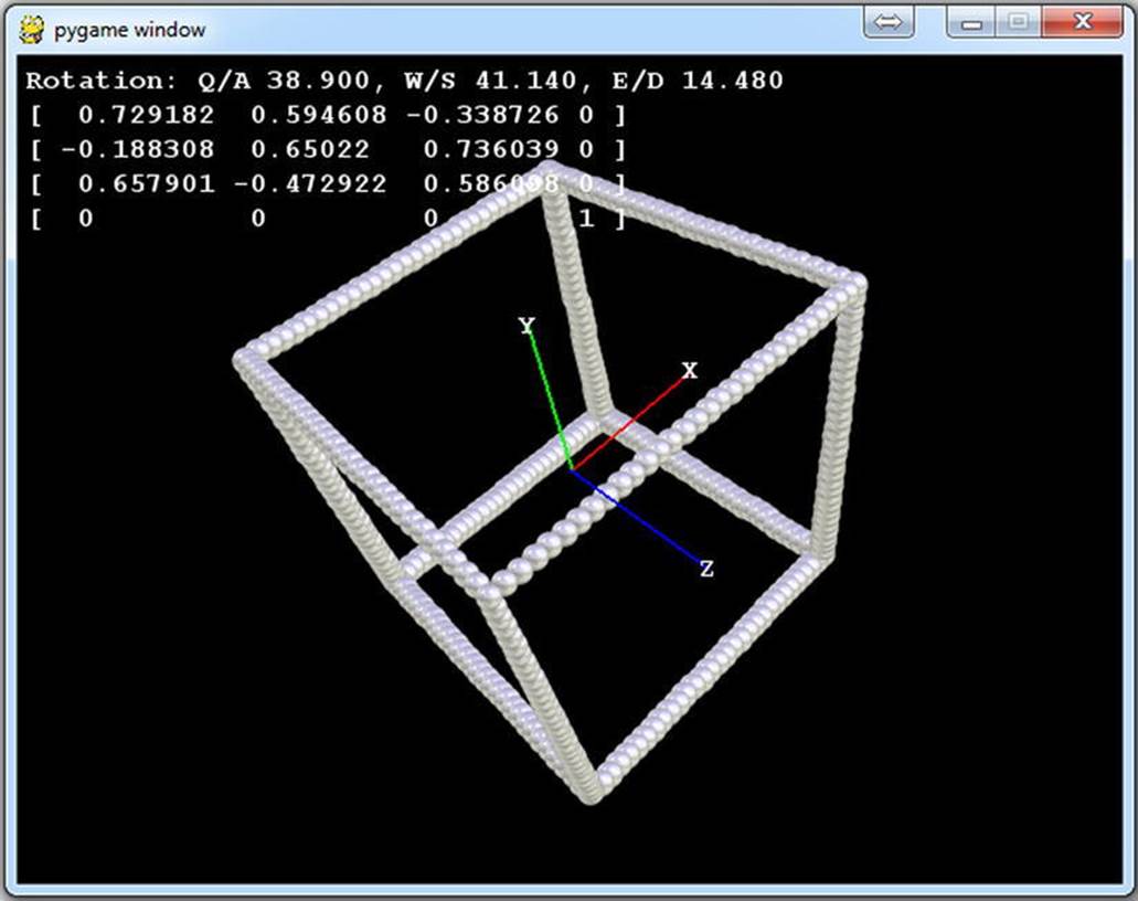
Figure 9-5. 3D transformations in action

Tip A quicker way to create a transformation about all three axes is to use the xyz_rotation function, which takes three angles.

Listing 9-3. Matrix Transformation in Action (rotation3d.py)

import pygame
from pygame.locals import *
from gameobjects.vector3 import Vector3
from gameobjects.matrix44 import Matrix44 as Matrix
from math import *
from random import randint

SCREEN_SIZE = (640, 480)
CUBE_SIZE = 300

def calculate_viewing_distance(fov, screen_width):

d = (screen_width/2.0) / tan(fov/2.0)
return d

def run():

pygame.init()
screen = pygame.display.set_mode(SCREEN_SIZE, 0)

font = pygame.font.SysFont("courier new", 16, True)

ball = pygame.image.load("ball.png").convert_alpha()

points = []

fov = 75. # Field of view
viewing_distance = calculate_viewing_distance(radians(fov), SCREEN_SIZE[0])

# Create a list of points along the edge of a cube
for x in range(0, CUBE_SIZE+1, 10):
edge_x = x == 0 or x == CUBE_SIZE

for y in range(0, CUBE_SIZE+1, 10):
edge_y = y == 0 or y == CUBE_SIZE

for z in range(0, CUBE_SIZE+1, 10):
edge_z = z == 0 or z == CUBE_SIZE

if sum((edge_x, edge_y, edge_z)) >= 2:

point_x = float(x) - CUBE_SIZE/2
point_y = float(y) - CUBE_SIZE/2
point_z = float(z) - CUBE_SIZE/2

points.append(Vector3(point_x, point_y, point_z))

def point_z(point):
return point[2]

center_x, center_y = SCREEN_SIZE
center_x /= 2
center_y /= 2

ball_w, ball_h = ball.get_size()
ball_center_x = ball_w / 2
ball_center_y = ball_h / 2

camera_position = Vector3(0.0, 0.0, 600.)

rotation = Vector3()
rotation_speed = Vector3(radians(20), radians(20), radians(20))

clock = pygame.time.Clock()

# Some colors for drawing
red = (255, 0, 0)
green = (0, 255, 0)
blue = (0, 0, 255)
white = (255, 255, 255)

# Labels for the axes
x_surface = font.render("X", True, white)
y_surface = font.render("Y", True, white)
z_surface = font.render("Z", True, white)

while True:

for event in pygame.event.get():
if event.type == QUIT:
pygame.quit()
quit()

screen.fill((0, 0, 0))

time_passed = clock.tick()
time_passed_seconds = time_passed / 1000.

rotation_direction = Vector3()

#Adjust the rotation direction depending on key presses
pressed_keys = pygame.key.get_pressed()

if pressed_keys[K_q]:
rotation_direction.x = +1.0
elif pressed_keys[K_a]:
rotation_direction.x = -1.0

if pressed_keys[K_w]:
rotation_direction.y = +1.0
elif pressed_keys[K_s]:
rotation_direction.y = -1.0

if pressed_keys[K_e]:
rotation_direction.z = +1.0
elif pressed_keys[K_d]:
rotation_direction.z = -1.0

# Apply time based movement to rotation
rotation += rotation_direction * rotation_speed * time_passed_seconds

# Build the rotation matrix
rotation_matrix = Matrix.x_rotation(rotation.x)
rotation_matrix *= Matrix.y_rotation(rotation.y)
rotation_matrix *= Matrix.z_rotation(rotation.z)

transformed_points = []

# Transform all the points and adjust for camera position
for point in points:

p = rotation_matrix.transform_vec3(point) - camera_position

transformed_points.append(p)

transformed_points.sort(key=point_z)

# Perspective project and blit all the points
for x, y, z in transformed_points:

if z < 0:
x = center_x + x * -viewing_distance / z
y = center_y + -y * -viewing_distance / z

screen.blit(ball, (x-ball_center_x, y-ball_center_y))

# Function to draw a single axes, see below
def draw_axis(color, axis, label):

axis = rotation_matrix.transform_vec3(axis * 150.)
SCREEN_SIZE = (640, 480)
center_x = SCREEN_SIZE[0] / 2.0
center_y = SCREEN_SIZE[1] / 2.0
x, y, z = axis - camera_position

x = center_x + x * -viewing_distance / z
y = center_y + -y * -viewing_distance / z

pygame.draw.line(screen, color, (center_x, center_y), (x, y), 2)

w, h = label.get_size()
screen.blit(label, (x-w/2, y-h/2))

# Draw the x, y and z axes
x_axis = Vector3(1, 0, 0)
y_axis = Vector3(0, 1, 0)
z_axis = Vector3(0, 0, 1)

draw_axis(red, x_axis, x_surface)
draw_axis(green, y_axis, y_surface)
draw_axis(blue, z_axis, z_surface)

# Display rotation information on screen
degrees_txt = tuple(degrees(r) for r in rotation)
rotation_txt = "Rotation: Q/A %.3f, W/S %.3f, E/D %.3f" % degrees_txt
txt_surface = font.render(rotation_txt, True, white)
screen.blit(txt_surface, (5, 5))

# Displat the rotation matrix on screen
matrix_txt = str(rotation_matrix)
txt_y = 25
for line in matrix_txt.split('\n'):
txt_surface = font.render(line, True, white)
screen.blit(txt_surface, (5, txt_y))
txt_y += 20

pygame.display.update()

if __name__ == "__main__":
run()

The matrices in Listing 9-3 transform the points of a cube to their final positions onscreen. Games do many such transforms in the process of rendering a 3D world, and have more sophisticated graphics than can be produced with 2D sprites. In the following section, you will learn how tojoin up the points in a model and use lighting to create solid-looking 3D models.

Introducing OpenGL

Today’s graphics cards come with chips that are dedicated to the task of drawing 3D graphics, but that wasn’t always the case; in the early days of 3D games on home computers, the programmer had to write code to draw the graphics for each game. Drawing polygons (shapes used in games) in software is time consuming, as the processor has to calculate each pixel individually. When graphics cards with 3D acceleration became popular, they freed up the processor to do work on other aspects of the game, such as artificial intelligence, resulting in better-looking games with richer gameplay.

OpenGL is an application programming interface (API) for working with the 3D capabilities of graphics cards. There are other APIs for 3D, but we will be using OpenGL, because it is well supported across platforms; OpenGL-powered games can be made to run on many different computers and consoles. It comes installed by default on all major platforms that Pygame runs on, usually as part of your graphics drivers.

There is a downside to using OpenGL with Pygame. With an OpenGL game, you can’t blit from a surface to the screen, or draw directly to it with any of the pygame.draw functions. You can use any of the other Pygame modules that don’t draw to the screen, such as pygame.key,pygame.time, and pygame.image. The event loop and general structure of a Pygame script doesn’t change when using OpenGL, so you can still apply what you have learned in the previous chapters.

Installing PyOpenGL

Although OpenGL is probably already on your system, you will still need to install PyOpenGL, which is a module that interfaces the OpenGL drivers on your computer with the Python language. You can install PyOpenGL with pip, by opening cmd.exe, bash, or the shell you happen to use and doing:

pip install PyOpenGL

For more information regarding PyOpenGL, see the project’s website at http://pyopengl.sourceforge.net/. For the latest news on OpenGL, see http://www.opengl.org/.

Tip Easy Install is a very useful tool, because it can find and install a huge number of Python modules automatically.

Initializing OpenGL

The PyOpenGL module consists of a number of functions, which can be imported with a single line:

from OpenGL.GL import *

This line imports the OpenGL functions, which begin with gl, for example, glVertex, which we will cover later. To get started using PyOpenGL with PyGame, you will almost always need the following imports:

from OpenGL.GL import *
from OpenGL.GLU import *
import pygame
from pygame.locals import *

pygame.locals contains some of the screen definitions that we’ll be using, OpenGL.GL and OpenGL.GLU are the core OpenGL modules.

Before you can use any of the functions in these modules, you must first tell Pygame to create an OpenGL display surface. Although this surface is different from a typical 2D display surface, it is created in the usual way with the pygame.display.set_mode function. The following line creates a 640 × 480 OpenGL surface called screen:

screen = pygame.display.set_mode((640, 480), HWSURFACE|OPENGL|DOUBLEBUF)

The OPENGL flag tells Pygame to create an OpenGL surface; HWSURFACE creates it in hardware, which is important for accelerated 3D; and DOUBLEBUF makes it double-buffered, which reduces flickering. You may also want to add FULLSCREEN to expand the display to fill the entire screen, but it is convenient to work in windowed mode when developing.

OpenGL Primer

OpenGL contains several matrices that are applied to the coordinates of what you draw to the screen. The two that are most commonly used are called GL_PROJECTION and GL_MODELVIEW. The projection matrix (GL_PROJECTION) takes a 3D coordinate and projects it onto 2D space so that it can be rendered to the screen. We’ve been doing this step manually in our experiments with 3D—it basically does the multiplication by the view distance and divides by the z component. The model view matrix is actually a combination of two matrices: the model matrix transforms (translates, scales, rotates, etc.) the model to its position in the world and the view matrix adjusts the objects to be relative to the camera (usually the player character’s viewpoint).

Resizing the Display

Before we begin drawing anything to the screen, we first have to tell OpenGL about the dimensions of the display and set up the GL_PROJECTION and GL_MODELVIEW matrices (see Listing 9-4).

Listing 9-4. Resizing the Viewport

def resize(width, height):
glViewport(0, 0, width, height)
glMatrixMode(GL_PROJECTION)
glLoadIdentity()
gluPerspective(60, float(width)/height, 1, 10000)
glMatrixMode(GL_MODELVIEW)
glLoadIdentity()

The resize function in Listing 9-4 takes the width and height of the screen, and should be called when the display is initialized or the screen dimensions change. The call to glViewport tells OpenGL that we want to use the area of the screen from coordinate (0, 0), with a size of (width, height), that is, the entire screen. The next line calls glMatrixMode(GL_PROJECTION), which tells OpenGL that all further calls that work with matrices will apply to the projection matrix. It is followed by a call to glLoadIdentity, which resets the projection matrix to identity, and a call to gluPerspective (from the GLU library), which sets a standard perspective projection matrix. This function takes four parameters: the field of view of the camera, the aspect ratio (width divided by height), followed by the near and far clipping planes. These clipping planes define the range of distances that can be “seen”; anything outside that range won’t be visible to the player. The viewable area in the 3D screen is called the viewing frustum (see Figure 9-6), which resembles a pyramid with a portion of the top cut off.

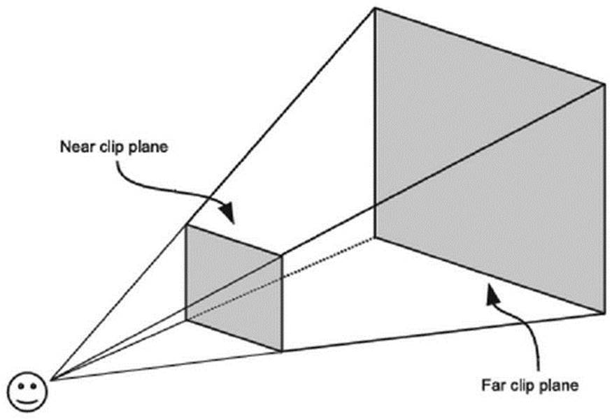
Figure 9-6. The viewing frustum

Initializing OpenGL Features

The resize function is enough to start using OpenGL functions to render to the screen, but there are a few other things we should set to make it more interesting (see Listing 9-5).

Listing 9-5. Initializing OpenGL

def init():

glEnable(GL_DEPTH_TEST)
glClearColor(1.0, 1.0, 1.0, 0.0)

glShadeModel(GL_FLAT)
glEnable(GL_COLOR_MATERIAL)

glEnable(GL_LIGHTING)
glEnable(GL_LIGHT0)
glLight(GL_LIGHT0, GL_POSITION, (0, 1, 1, 0))

The first thing that the init function does is call glEnable with GL_DEPTH_TEST, which tells OpenGL to enable the Z buffer. This ensures that objects that are far from the camera aren’t drawn over objects that are near to the camera, regardless of the order that we draw them in code.

The glEnable function is used to enable OpenGL features, and glDisable is used to disable them. Both functions take one of a number of uppercase constants, beginning with GL_. We will cover a number of these that you can use in your games in this book, but see the OpenGL documentation for a complete list.

The second line in init sets the clear color, which is the color of the parts of the screen that aren’t drawn to (the equivalent of automatically calling screen.fill in the 2D sample code). In OpenGL, colors are given as four values for the red, green, blue, and alpha components, but rather than a value between 0 and 255, it uses values between 0 and 1.

The remaining lines in the function initialize OpenGL’s lighting capabilities, which automatically shade 3D objects depending on the position of a number of lights in the 3D world. The call to glShadeModel sets the shade model to GL_FLAT, which is used to shade faceted objects such as cubes, or anything with edged surfaces. An alternative setting for the shade model is GL_SMOOTH, which is better for shading curved objects. The call to glEnable(GL_COLOR_MATERIAL) tells OpenGL that we want to enable materials, which are settings that define how a surface interacts with a light source. For instance, we could make a sphere appear highly polished like marble, or softer like a piece of fruit, by adjusting its material properties.

The remaining portion of Listing 9-5 enables lighting (glEnable(GL_LIGHTING)) and light zero (glEnable(GL_LIGHT0)). There are a number of different lights that you can switch on in OpenGL; they are numbered GL_LIGHT0, GL_LIGHT1, GL_LIGHT2, and so on. In a game, you would have at least one light (probably for the sun), and additional lights for other things such as headlights, lamps, or special effects. Placing a light source inside a fireball effect, for example, will ensure that it illuminates the surrounding terrain.

The last line sets the position of light zero to (0, 1, 1, 0). The first three values in this tuple are the x, y, and z coordinates of the light; the last value tells OpenGL to make it a directional light, which creates a light source with parallel light rays, similar to the sun. If the last value is 1, OpenGL creates a point light source, which looks like a close-up light, such as a bulb, candle, or plasma fireball. See Figure 9-7 for the differences between point and directional light sources.

Tip You can get the number of lights that your OpenGL driver supports with glGetInteger(GL_MAX_LIGHTS). Typically you will get eight, but it can vary depending on your platform.

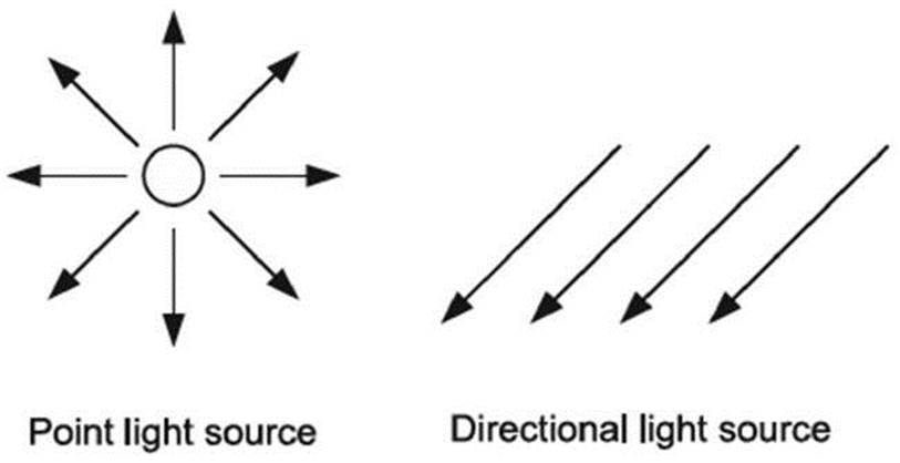
Figure 9-7. OpenGL light sources

Drawing in Three Dimensions

Now that we have initialized OpenGL and created a light source, we can start drawing 3D shapes. OpenGL supports a number of primitives that you can use to build a 3D scene, such as points, lines, and triangles. Each takes a number of pieces of information, depending on the type of primitive and the OpenGL features that are enabled. Because of this, there aren’t single functions for each primitive as there are in 2D Pygame. The information is given in a number of function calls, and when OpenGL has all the information it needs, it can draw the primitive.

To draw a primitive in OpenGL, first call glBegin, with one of the primitive constants (see Table 9-2). Next, send OpenGL the information it needs to draw the primitive. At a minimum it will need a number of 3D points, specified with the glVertex function (a vertex is a point that forms part of a shape), but you can give it other information, such as color with the glColor function. Once all the information has been given, call glEnd, which tells OpenGL that all the information has been provided and it can be used to draw the primitive.

Note The call to glVertex should always come after other information for a vertex is given.

Table 9-2. OpenGL Primitives

Listing 9-6 is an example of how you might draw a red square with OpenGL. The first line tells OpenGL that you want to draw quads (shapes with four points). The next line sends the color red (1.0, 0.0, 0.0), so all vertices will be red until the next call to glColor. The four calls toglVertex send the coordinates of each of the corners of the square, and finally, the call to glEnd tells OpenGL that you have finished sending vertex information. With four vertices, OpenGL can draw a single quad, but if you were to give it more, it would draw a quad for every four vertices you send it.

Listing 9-6. Pseudocode for Drawing a Red Square

glBegin(GL_QUADS)
glColor(1.0, 0.0, 0.0) # Red
glVertex(100.0, 100.0, 0.0) # Top left
glVertex(200.0, 100.0, 0.0) # Top right
glVertex(200.0, 200.0, 0.0) # Bottom right
glVertex(100.0, 200.0, 0.0) # Bottom left

glEnd()

Normals

If you have OpenGL lighting enabled, you will need to send an additional piece of information for primitives called a normal, which is a unit vector (a vector of length 1.0) that faces outward from a 3D shape. This vector is necessary for calculating the shading from lights in the scene. For example, if you have a cube in the center of the screen aligned along the axis, the normal for the front face is (0, 0, 1) because it is facing along the positive z axis, and the normal for the right face is (1, 0, 0) because it faces along the x axis (see Figure 9-8).

To send a normal to OpenGL, use the glNormal3d function, which takes three values for the normal vector, or the glNormal3dv function, which takes a sequence of three values. For example, if the square in Listing 9-6 was the front face of a cube you would set the normal withglNormal3d(0, 0, 1) or glNormal3dv(front_vector). The latter is useful because it can be used with Vector3 objects. If you are using flat shading (glShadeModel(GL_FLAT)), you will need one normal per face. For smooth shading (glShadeModel(GL_SMOOTH)), you will need to supply a normal per vertex.

Figure 9-8. Normals of a cube

Display Lists

If you have many primitives to draw—which is typically the case for a 3D game—then it can be slow to make all the calls necessary to draw them all. It is faster to send many primitives to OpenGL in one go, rather than one at a time. There are several ways of doing this, but one of the easiest ways is to use display lists.

You can think of a display list as a number of OpenGL function calls that have been recorded and can be played back at top speed. To create a display list, first call glGenLists(1), which returns an id value to identify the display list. Then call glNewList with the id and the constant GL_COMPILE, which begins compiling the display list. When you have finished sending primitives to OpenGL, call glEndList to end the compile process. Once you have compiled the display list, call glCallList with the id to draw the recorded primitives at maximum speed. Display lists will let you create games that run as fast as commercial products, so it is a good idea to get into the habit of using them! Listing 9-7 is an example of how you might create a display list to draw a tank model. It assumes that there is a function draw_tank, which sends the primitives to OpenGL.

Once you have created a display list, you can draw it many times in the same scene by setting a different transformation matrix before each call to glCallList(tank_display_id).

Listing 9-7. Creating a Display List

# Create a display list
tank_display_list = glGenLists(1)
glNewList(tank_display_list, GL_COMPILE)

draw_tank()

# End the display list
glEndList()

Storing a 3D Model

3D objects are a collection of primitives, typically either triangles or quads, which form part of a larger shape. For instance, a cube can be created with six quads, one for each side. More complex shapes, particularly organic shapes like people or bug-eyed aliens, take many more primitives to create. The most efficient way to store a model is to keep a list of vertices, and additional information about which points to use to draw the faces (primitives). For instance, a cube could be stored as six vertices (one for each corner), and the faces would be stored as four indexes into that list (see Figure 9-9).

This is typically how models are stored in files produced by 3D editing software. Although there are a variety of different formats, they will all contain a list of vertices and a list of indices that connect vertices with primitives. We’ll cover how to read these models later in this book.

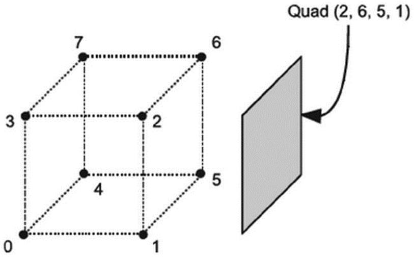
Figure 9-9. Faces and vertices

Seeing OpenGL in Action

We’ve covered enough theory for one chapter; let’s put what we have learned into practice. We are going to use OpenGL to create a very simple world composed of cubes, and give the player the ability to fly around and explore it.

When you run Listing 9-8, you will find yourself in a colorful maze. Use the left and right cursor keys to pan around, and the Q and A keys to move forward and back. The effect is much like a first-person shooter, but if you press the up or down cursor key, you will find that you can actually fly above, or below, the 3D world (see Figure 9-10). If you press the Z or X key, you can also roll the camera.

So how is this world created? The Map class in Listing 9-8 reads in a small bitmap (map.png) and goes through each pixel. When it finds a nonwhite pixel, it creates a colored cube at a corresponding point in 3D. The Cube class contains a list of vertices, normals, and normal indicesthat define which vertices are used in each side of the cube, and it uses this information to draw the six sides.

The whole world is transformed with a single camera matrix (camera_matrix), which is modified as the user presses keys. This matrix is multiplied by a rotation matrix when the user rotates the camera, and the translate row is adjusted to move the camera forward and back. Both rotation and translation use the familiar time-based calculations to give a consistent speed.

Before the 3D world is rendered, we must send the camera matrix to OpenGL. The following line uploads the camera matrix to OpenGL:

glLoadMatrixd(camera_matrix.get_inverse().to_opengl())

The get_inverse function returns the inverse of the matrix, which is a matrix that does the exact opposite of the original. The reason we use the inverse, and not the original, is because we want to transform everything in the world to be relative to the camera. To explain it another way, if you are looking directly at an object and you turn your head to the right, that object is now on the left side of your vision. It’s the same with the camera matrix; the world is transformed in the opposite way.

The to_opengl function of Matrix44 converts the matrix into a single list, which is the format that the glLostMatrixd requires to send the matrix to OpenGL. Once that matrix has been sent, everything in the 3D world will be transformed to be relative to the camera.

Note It may seem a little odd, but when you move a camera about in a 3D world, you are actually transforming the world and not the camera!

Figure 9-10. Cube world

Listing 9-8. Flying Around Cube World! (firstopengl.py)

from math import radians

from OpenGL.GL import *
from OpenGL.GLU import *

import pygame
from pygame.locals import *

from gameobjects.matrix44 import *
from gameobjects.vector3 import *

SCREEN_SIZE = (800, 600)

def resize(width, height):

glViewport(0, 0, width, height)
glMatrixMode(GL_PROJECTION)
glLoadIdentity()
gluPerspective(60.0, float(width)/height, .1, 1000.)
glMatrixMode(GL_MODELVIEW)
glLoadIdentity()

def init():

glEnable(GL_DEPTH_TEST)

glShadeModel(GL_FLAT)
glClearColor(1.0, 1.0, 1.0, 0.0)

glEnable(GL_COLOR_MATERIAL)

glEnable(GL_LIGHTING)
glEnable(GL_LIGHT0)
glLight(GL_LIGHT0, GL_POSITION, (0, 1, 1, 0))

class Cube(object):

def __init__(self, position, color):

self.position = position
self.color = color

# Cube information

num_faces = 6

vertices = [ (0.0, 0.0, 1.0),
(1.0, 0.0, 1.0),
(1.0, 1.0, 1.0),
(0.0, 1.0, 1.0),
(0.0, 0.0, 0.0),
(1.0, 0.0, 0.0),
(1.0, 1.0, 0.0),
(0.0, 1.0, 0.0) ]

normals = [ (0.0, 0.0, +1.0), # front
(0.0, 0.0, -1.0), # back
(+1.0, 0.0, 0.0), # right
(-1.0, 0.0, 0.0), # left
(0.0, +1.0, 0.0), # top
(0.0, -1.0, 0.0) ] # bottom

vertex_indices = [ (0, 1, 2, 3), # front
(4, 5, 6, 7), # back
(1, 5, 6, 2), # right
(0, 4, 7, 3), # left
(3, 2, 6, 7), # top
(0, 1, 5, 4) ] # bottom

def render(self):

# Set the cube color, applies to all vertices till next call
glColor( self.color )

# Adjust all the vertices so that the cube is at self.position
vertices = []
for v in self.vertices:
vertices.append( tuple(Vector3(v)+ self.position) )

# Draw all 6 faces of the cube
glBegin(GL_QUADS)

for face:no in range(self.num_faces):

glNormal3dv( self.normals[face:no] )

v1, v2, v3, v4 = self.vertex_indices[face:no]

glVertex( vertices[v1] )
glVertex( vertices[v2] )
glVertex( vertices[v3] )
glVertex( vertices[v4] )

glEnd()

class Map(object):

def __init__(self):

map_surface = pygame.image.load("map.png")
map_surface.lock()

w, h = map_surface.get_size()

self.cubes = []

# Create a cube for every non-white pixel
for y in range(h):
for x in range(w):

r, g, b, a = map_surface.get_at((x, y))

if (r, g, b) != (255, 255, 255):

gl_col = (r/255.0, g/255.0, b/255.0)
position = (float(x), 0.0, float(y))
cube = Cube( position, gl_col )
self.cubes.append(cube)

map_surface.unlock()

self.display_list = None

def render(self):

if self.display_list is None:

# Create a display list
self.display_list = glGenLists(1)
glNewList(self.display_list, GL_COMPILE)

# Draw the cubes
for cube in self.cubes:
cube.render()

# End the display list
glEndList()

else:

# Render the display list
glCallList(self.display_list)

def run():

pygame.init()
screen = pygame.display.set_mode(SCREEN_SIZE, HWSURFACE|OPENGL|DOUBLEBUF)

resize(*SCREEN_SIZE)
init()

clock = pygame.time.Clock()

# This object renders the 'map'
map = Map()

# Camera transform matrix
camera_matrix = Matrix44()
camera_matrix.translate = (10.0, .6, 10.0)

# Initialize speeds and directions
rotation_direction = Vector3()
rotation_speed = radians(90.0)
movement_direction = Vector3()
movement_speed = 5.0

while True:

for event in pygame.event.get():
if event.type == QUIT:
pygame.quit()
quit()
if event.type == KEYUP and event.key == K_ESCAPE:
pygame.quit()
quit()

# Clear the screen, and z-buffer
glClear(GL_COLOR_BUFFER_BIT | GL_DEPTH_BUFFER_BIT);

time_passed = clock.tick()
time_passed_seconds = time_passed / 1000.

pressed = pygame.key.get_pressed()

# Reset rotation and movement directions
rotation_direction.set(0.0, 0.0, 0.0)
movement_direction.set(0.0, 0.0, 0.0)

# Modify direction vectors for key presses
if pressed[K_LEFT]:
rotation_direction.y = +1.0
elif pressed[K_RIGHT]:
rotation_direction.y = -1.0
if pressed[K_UP]:
rotation_direction.x = -1.0
elif pressed[K_DOWN]:
rotation_direction.x = +1.0
if pressed[K_z]:
rotation_direction.z = -1.0
elif pressed[K_x]:
rotation_direction.z = +1.0
if pressed[K_q]:
movement_direction.z = -1.0
elif pressed[K_a]:
movement_direction.z = +1.0

# Calculate rotation matrix and multiply by camera matrix
rotation = rotation_direction * rotation_speed * time_passed_seconds
rotation_matrix = Matrix44.xyz_rotation(*rotation)
camera_matrix *= rotation_matrix

# Calcluate movment and add it to camera matrix translate
heading = Vector3(camera_matrix.forward)
movement = heading * movement_direction.z * movement_speed
camera_matrix.translate += movement * time_passed_seconds

# Upload the inverse camera matrix to OpenGL
glLoadMatrixd(camera_matrix.get_inverse().to_opengl())

# Light must be transformed as well
glLight(GL_LIGHT0, GL_POSITION, (0, 1.5, 1, 0))

# Render the map
map.render()

# Show the screen
pygame.display.flip()

if __name__ == "__main__":
run()

Summary

We’ve covered a lot of ground with this chapter. We started out with matrices, which are an important topic because they are used everywhere in 3D games, including handhelds and consoles. The math for working with matrices can be intimidating, but if you use a prebuilt matrix class, such as gameobjects.Matrix44, you won’t need to know the details of how they work (most game programmers aren’t mathematicians)! It’s more important that you know how to combine translation, rotation, and scaling to manipulate objects in a game. Visualizing a matrix from its grid of numbers is also a useful skill to have, and will help you fix bugs if anything goes wrong with your games.

You also learned how to work with OpenGL to create 3D visuals. OpenGL is a large, powerful API, and we have only touched on a portion of it. We covered the basics of how to store a 3D model and send it to OpenGL for rendering, which we can make use of even when more OpenGL features are enabled. Later chapters will describe how to add textures and transparency to create visuals that will really impress!

Listing 9-8 is a good starting point for any experiments with OpenGL. Try tweaking some of the values to produce different effects, or add more interesting shapes to the cube world. You could even turn it into a game by adding a few enemies (see Chapter 7).

In the next chapter we will take a break from 3D to explore how you can use sound with Pygame.