High Performance Python (2014)

Chapter 11. Using Less RAM

QUESTIONS YOU’LL BE ABLE TO ANSWER AFTER THIS CHAPTER

§ Why should I use less RAM?

§ Why are numpy and array better for storing lots of numbers?

§ How can lots of text be efficiently stored in RAM?

§ How could I count (approximately!) to 1e77 using just 1 byte?

§ What are Bloom filters and why might I need them?

We rarely think about how much RAM we’re using until we run out of it. If you run out while scaling your code, it can become a sudden blocker. Fitting more into a machine’s RAM means fewer machines to manage, and it gives you a route to planning capacity for larger projects. Knowing why RAM gets eaten up and considering more efficient ways to use this scarce resource will help you deal with scaling issues.

Another route to saving RAM is to use containers that utilize features in your data for compression. In this chapter, we’ll look at tries (ordered tree data structures) and a DAWG that can compress a 1.1 GB set of strings down to just 254 MB with little change in performance. A third approach is to trade storage for accuracy. For this we’ll look at approximate counting and approximate set membership, which use dramatically less RAM than their exact counterparts.

A consideration with RAM usage is the notion that “data has mass.” The more there is of it, the slower it moves around. If you can be parsimonious in your use of RAM your data will probably get consumed faster, as it’ll move around buses faster and more of it will fit into constrained caches. If you need to store it in offline storage (e.g., a hard drive or a remote data cluster), then it’ll move far more slowly to your machine. Try to choose appropriate data structures so all your data can fit onto one machine.

Counting the amount of RAM used by Python objects is surprisingly tricky. We don’t necessarily know how an object is represented behind the scenes, and if we ask the operating system for a count of bytes used it will tell us about the total amount allocated to the process. In both cases, we can’t see exactly how each individual Python object adds to the total.

As some objects and libraries don’t report their full internal allocation of bytes (or they wrap external libraries that do not report their allocation at all), this has to be a case of best-guessing. The approaches explored in this chapter can help us to decide on the best way to represent our data so we use less RAM overall.

Objects for Primitives Are Expensive

It’s common to work with containers like the list, storing hundreds or thousands of items. As soon as you store a large number, RAM usage becomes an issue.

A list with 100,000,000 items consumes approximately 760 MB of RAM, if the items are the same object. If we store 100,000,000 different items (e.g., unique integers), then we can expect to use gigabytes of RAM! Each unique object has a memory cost.

In Example 11-1, we store many 0 integers in a list. If you stored 100,000,000 references to any object (regardless of how large one instance of that object was), you’d still expect to see a memory cost of roughly 760 MB as the list is storing references to (not copies of) the object. Refer back to Using memory_profiler to Diagnose Memory Usage for a reminder on how to use memory_profiler; here we load it as a new magic function in IPython using %load_ext memory_profiler.

Example 11-1. Measuring memory usage of 100,000,000 of the same integer in a list

In [1]: %load_ext memory_profiler # load the %memit magic function

In [2]: %memit [0]*int(1e8)

peak memory: 790.64 MiB, increment: 762.91 MiB

For our next example, we’ll start with a fresh shell. As the results of the first call to memit in Example 11-2 reveal, a fresh IPython shell consumes approximately 20 MB of RAM. Next, we can create a temporary list of 100,000,000 unique numbers. In total, this consumes approximately 3.1 GB.

WARNING

Memory can be cached in the running process, so it is always safer to exit and restart the Python shell when using memit for profiling.

After the memit command finishes, the temporary list is deallocated. The final call to memit shows that the memory usage stays at approximately 2.3 GB.

TIP

Before reading the answer, why might the Python process still hold 2.3 GB of RAM? What’s left behind, even though the list has gone to the garbage collector?

Example 11-2. Measuring memory usage of 100,000,000 different integers in a list

# we use a new IPython shell so we have a clean memory

In [1]: %load_ext memory_profiler

In [2]: %memit # show how much RAM this process is consuming right now

peak memory: 20.05 MiB, increment: 0.03 MiB

In [3]: %memit [n for n inxrange(int(1e8))]

peak memory: 3127.53 MiB, increment: 3106.96 MiB

In [4]: %memit

peak memory: 2364.81 MiB, increment: 0.00 MiB

The 100,000,000 integer objects occupy the majority of the 2.3 GB, even though they’re no longer being used. Python caches primitive objects like integers for later use. On a system with constrained RAM this can cause problems, so you should be aware that these primitives may build up in the cache.

A subsequent memit in Example 11-3 to create a second 100,000,000-item list consumes approximately 760 MB; this takes the overall allocation during this call back up to approximately 3.1 GB. The 760 MB is for the container alone, as the underlying Python integer objects already exist—they’re in the cache, so they get reused.

Example 11-3. Measuring memory usage again for 100,000,000 different integers in a list

In [5]: %memit [n for n inxrange(int(1e8))]

peak memory: 3127.52 MiB, increment: 762.71 MiB

Next, we’ll see that we can use the array module to store 100,000,000 integers far more cheaply.

The Array Module Stores Many Primitive Objects Cheaply

The array module efficiently stores primitive types like integers, floats, and characters, but not complex numbers or classes. It creates a contiguous block of RAM to hold the underlying data.

In Example 11-4, we allocate 100,000,000 integers (8 bytes each) into a contiguous chunk of memory. In total, approximately 760 MB is consumed by the process. The difference between this approach and the previous list-of-unique-integers approach is 2300MB - 760MB == 1.5GB. This is a huge savings in RAM.

Example 11-4. Building an array of 100,000,000 integers with 760 MB of RAM

In [1]: %load_ext memory_profiler

In [2]: import array

In [3]: %memit array.array('l', xrange(int(1e8)))

peak memory: 781.03 MiB, increment: 760.98 MiB

In [4]: arr = array.array('l')

In [5]: arr.itemsize

Out[5]: 8

Note that the unique numbers in the array are not Python objects; they are bytes in the array. If we were to dereference any of them, then a new Python int object would be constructed. If you’re going to compute on them no overall saving will occur, but if instead you’re going to pass the array to an external process or use only some of data, you should see a good savings in RAM compared to using a list of integers.

NOTE

If you’re working with a large array or matrix of numbers with Cython and you don’t want an external dependency on numpy, be aware that you can store your data in an array and pass it into Cython for processing without any additional memory overhead.

The array module works with a limited set of datatypes with varying precisions (see Example 11-5). Choose the smallest precision that you need, so you allocate just as much RAM as needed and no more. Be aware that the byte size is platform-dependent—the sizes here refer to a 32-bit platform (it states minimum size) while we’re running the examples on a 64-bit laptop.

Example 11-5. The basic types provided by the array module

In [5]: array? # IPython magic, similar to help(array)

Type: module

String Form:<module 'array' (built-in)>

Docstring:

This module defines an object type which can efficiently represent

an array of basic values: characters, integers, floating point

numbers. Arrays are sequence types andbehave very much like lists,

except that the type of objects stored inthem isconstrained. The

type isspecified at object creation time by using a type code, which

is a single character. The following type codes are defined:

Type code C Type Minimum size inbytes

'c' character 1

'b' signed integer 1

'B' unsigned integer 1

'u' Unicode character 2

'h' signed integer 2

'H' unsigned integer 2

'i' signed integer 2

'I' unsigned integer 2

'l' signed integer 4

'L' unsigned integer 4

'f' floating point 4

'd' floating point 8

The constructor is:

array(typecode [, initializer]) -- create a new array

numpy has arrays that can hold a wider range of datatypes—you have more control over the number of bytes per item, and you can use complex numbers and datetime objects. A complex128 object takes 16 bytes per item: each item is a pair of 8-byte floating-point numbers. You can’t store complex objects in a Python array, but they come for free with numpy. If you’d like a refresher on numpy, look back to Chapter 6.

In Example 11-6 you can see an additional feature of numpy arrays—you can query for the number of items, the size of each primitive, and the combined total storage of the underlying block of RAM. Note that this doesn’t include the overhead of the Python object (typically this is tiny in comparison to the data you store in the arrays).

Example 11-6. Storing more complex types in a numpy array

In [1]: %load_ext memory_profiler

In [2]: import numpy as np

In [3]: %memit arr=np.zeros(1e8, np.complex128)

peak memory: 1552.48 MiB, increment: 1525.75 MiB

In [4]: arr.size # same as len(arr)

Out[4]: 100000000

In [5]: arr.nbytes

Out[5]: 1600000000

In [6]: arr.nbytes/arr.size # bytes per item

Out[6]: 16

In [7]: arr.itemsize # another way of checking

Out[7]: 16

Using a regular list to store many numbers is much less efficient in RAM than using an array object. More memory allocations have to occur, which each take time; calculations also occur on larger objects, which will be less cache friendly, and more RAM is used overall, so less RAM is available to other programs.

However, if you do any work on the contents of the array in Python the primitives are likely to be converted into temporary objects, negating their benefit. Using them as a data store when communicating with other processes is a great use case for the array.

numpy arrays are almost certainly a better choice if you are doing anything heavily numeric, as you get more datatype options and many specialized and fast functions. You might choose to avoid numpy if you want fewer dependencies for your project, though Cython and Pythran work equally well with array and numpy arrays; Numba works with numpy arrays only.

Python provides a few other tools to understand memory usage, as we’ll see in the following section.

Understanding the RAM Used in a Collection

You may wonder if you can ask Python about the RAM that’s used by each object. Python’s sys.getsizeof(obj) call will tell us something about the memory used by an object (most, but not all, objects provide this). If you haven’t seen it before, then be warned that it won’t give you the answer you’d expect for a container!

Let’s start by looking at some primitive types. An int in Python is a variable-sized object; it starts as a regular integer and turns into a long integer if you count above sys.maxint (on Ian’s 64-bit laptop this is 9,223,372,036,854,775,807).

As a regular integer it takes 24 bytes (the object has a lot of overhead), and as a long integer it consumes 36 bytes:

In [1]: sys.getsizeof(int())

Out[1]: 24

In [2]: sys.getsizeof(1)

Out[2]: 24

In [3]: n=sys.maxint+1

In [4]: sys.getsizeof(n)

Out[4]: 36

We can do the same check for byte strings. An empty string costs 37 bytes, and each additional character adds 1 byte to the cost:

In [21]: sys.getsizeof(b"")

Out[21]: 37

In [22]: sys.getsizeof(b"a")

Out[22]: 38

In [23]: sys.getsizeof(b"ab")

Out[23]: 39

In [26]: sys.getsizeof(b"cde")

Out[26]: 40

When we use a list we see different behavior. getsizeof isn’t counting the cost of the contents of the list, just the cost of the list itself. An empty list costs 72 bytes, and each item in the list takes another 8 bytes on a 64-bit laptop:

# goes up in 8-byte steps rather than the 24 we might expect!

In [36]: sys.getsizeof([])

Out[36]: 72

In [37]: sys.getsizeof([1])

Out[37]: 80

In [38]: sys.getsizeof([1,2])

Out[38]: 88

This is more obvious if we use byte strings—we’d expect to see much larger costs than getsizeof is reporting:

In [40]: sys.getsizeof([b""])

Out[40]: 80

In [41]: sys.getsizeof([b"abcdefghijklm"])

Out[41]: 80

In [42]: sys.getsizeof([b"a", b"b"])

Out[42]: 88

getsizeof only reports some of the cost, and often just for the parent object. As noted previously, it also isn’t always implemented, so it can have limited usefulness.

A slightly better tool is asizeof, which will walk a container’s hierarchy and make a best guess about the size of each object it finds, adding the sizes to a total. Be warned that it is quite slow.

In addition to relying on guesses and assumptions, it also cannot count memory allocated behind the scenes (e.g., a module that wraps a C library may not report the bytes allocated in the C library). It is best to use this as a guide. We prefer to use memit, as it gives us an accurate count of memory usage on the machine in question.

You use asizeof as follows:

In [1]: %run asizeof.py

In [2]: asizeof([b"abcdefghijklm"])

Out[2]: 136

We can check the estimate it makes for a large list—here we’ll use 10,000,000 integers:

# this takes 30 seconds to run!

In [1]: asizeof([x for x inxrange(10000000)]) # 1e7 integers

Out[1]: 321528064

We can validate this estimate by using memit to see how the process grew. In this case, the numbers are very similar:

In [2]: %memit([x for x inxrange(10000000)])

peak memory: 330.64 MiB, increment: 310.62 MiB

Generally the asizeof process is slower than using memit, but asizeof can be useful when you’re analyzing small objects. memit is probably more useful for real-world applications, as the actual memory usage of the process is measured rather than inferred.

Bytes Versus Unicode

One of the compelling reasons to switch to Python 3.3+ is that Unicode object storage is significantly cheaper than it is in Python 2.7. If you mainly handle lots of strings and they eat a lot of RAM, definitely consider a move to Python 3.3+. You get this RAM saving absolutely for free.

In Example 11-7 we can see a 100,000,000-character sequence being built as a collection of bytes (this is the same as a regular str in Python 2.7) and as a Unicode object. The Unicode variant takes four times as much RAM. Every Unicode character costs the same higher price, regardless of the number of bytes required to represent the underlying data.

Example 11-7. Unicode objects are expensive in Python 2.7

In [1]: %load_ext memory_profiler

In [2]: %memit b"a" * int(1e8)

peak memory: 100.98 MiB, increment: 80.97 MiB

In [3]: %memit u"a" * int(1e8)

peak memory: 380.98 MiB, increment: 360.92 MiB

The UTF-8 encoding of a Unicode object uses one byte per ASCII character and more bytes for less frequently seen characters. Python 2.7 uses an equal number of bytes for a Unicode character regardless of the character’s prevalence. If you’re not sure about Unicode encodings versus Unicode objects, then go and watch Net Batchelder’s “Pragmatic Unicode, or, How Do I Stop the Pain?”

From Python 3.3, we have a flexible Unicode representation thanks to PEP 393. It works by observing the range of characters in the string and using a smaller number of bytes to represent the lower-order characters if possible.

In Example 11-8 you can see that the costs of the byte and Unicode versions of an ASCII character are the same, and that using a non-ASCII character (sigma) the memory usage only doubles—this is still better than the Python 2.7 situation.

Example 11-8. Unicode objects are far cheaper in Python 3.3+

Python 3.3.2+ (default, Oct 9 2013, 14:50:09)

IPython 1.2.0 -- An enhanced Interactive Python.

...

In [1]: %load_ext memory_profiler

In [2]: %memit b"a" * int(1e8)

peak memory: 91.77 MiB, increment: 71.41 MiB

In [3]: %memit u"a" * int(1e8)

peak memory: 91.54 MiB, increment: 70.98 MiB

In [4]: %memit u"Σ" * int(1e8)

peak memory: 174.72 MiB, increment: 153.76 MiB

Given that Unicode objects are the default in Python 3.3+, if you work with lots of string data you’ll almost certainly benefit from the upgrade. The lack of cheap string storage was a hindrance for some in the early Python 3.1+ days, but now, with PEP 393, this is absolutely not an issue.

Efficiently Storing Lots of Text in RAM

A common problem with text is that it occupies a lot of RAM—but if we want to test if we have seen strings before or count their frequency, then it is convenient to have them in RAM rather than paging them to and from a disk. Storing the strings naively is expensive, but tries and directed acyclic word graphs (DAWGs) can be used to compress their representation and still allow fast operations.

These more advanced algorithms can save you a significant amount of RAM, which means that you might not need to expand to more servers. For production systems, the savings can be huge. In this section we’ll look at compressing a set of strings costing 1.1 GB down to 254 MB using a trie, with only a small change in performance.

For this example, we’ll use a text set built from a partial dump of Wikipedia. This set contains 8,545,076 unique tokens from a portion of the English Wikipedia and takes up 111,707,546 (111 MB) on disk.

The tokens are split on whitespace from their original articles; they have variable length and contain Unicode characters and numbers. They look like:

faddishness

'melanesians'

Kharálampos

PizzaInACup™

url="http://en.wikipedia.org/wiki?curid=363886"

VIIIa),

Superbagnères.

We’ll use this text sample to test how quickly we can build a data structure holding one instance of each unique word, and then we’ll see how quickly we can query for a known word (we’ll use the uncommon “Zwiebel,” from the painter Alfred Zwiebel). This lets us ask, “Have we seen Zwiebel before?” Token lookup is a common problem, and being able to do it quickly is important.

NOTE

When you try these containers on your own problems, be aware that you will probably see different behaviors. Each container builds its internal structures in different ways; passing in different types of token is likely to affect the build time of the structure, and different lengths of token will affect the query time. Always test in a methodical way.

Trying These Approaches on 8 Million Tokens

Figure 11-1 shows the 8-million-token text file (111 MB raw data) stored using a number of containers that we’ll discuss in this section. The x-axis shows RAM usage for each container, the y-axis tracks the query time, and the size of each point relates to the time taken to build the structure (larger means it took longer).

As we can see in this diagram, the set and DAWG examples use a lot of RAM. The list example is expensive on RAM and slow. The Marisa trie and HAT trie examples are the most efficient for this dataset; they use a quarter of the RAM of the other approaches with little change in lookup speed.

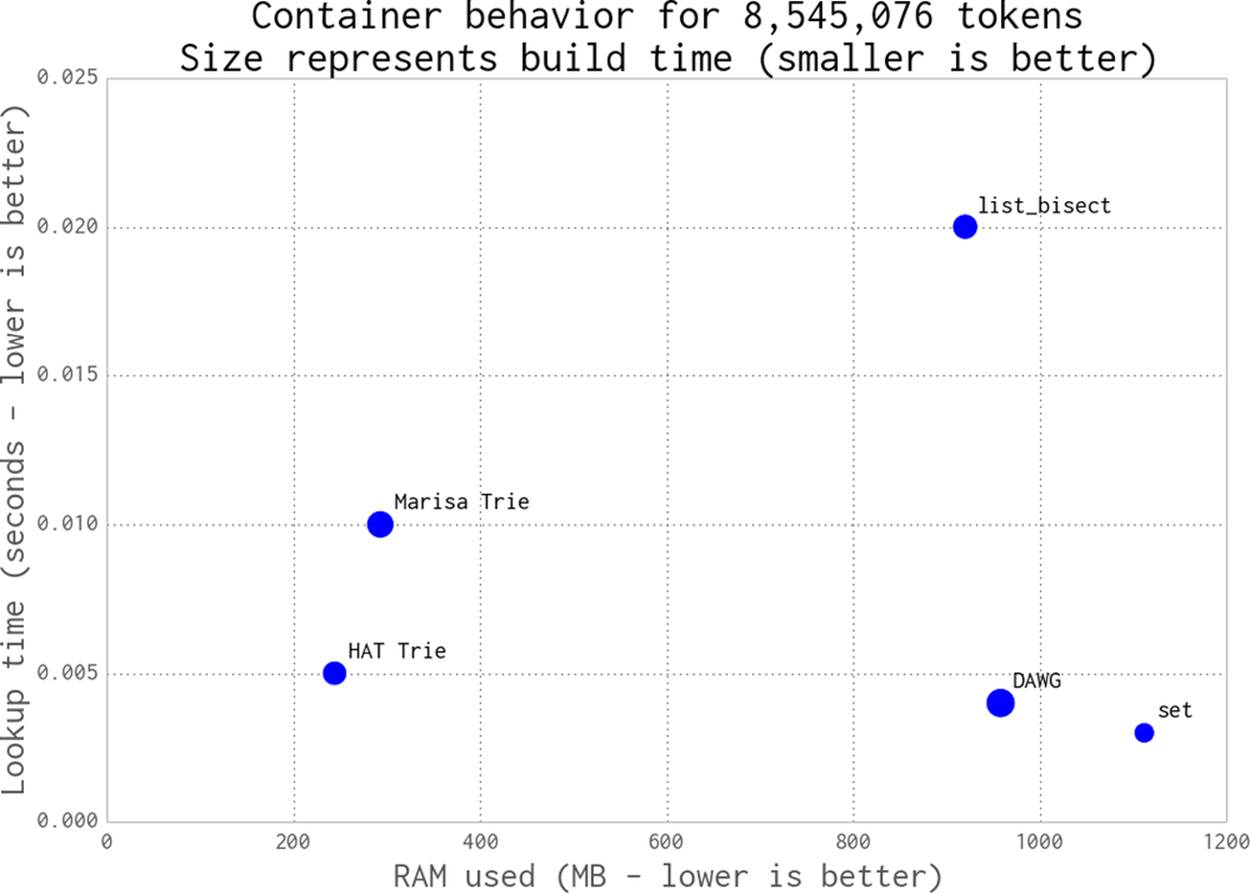
Figure 11-1. DAWG and tries versus built-in containers

The figure doesn’t show the lookup time for the naive list without sort approach, which we’ll introduce shortly, as it takes far too long. The datrie example is not included in the plot, because it raised a segmentation fault (we’ve had problems with it on other tasks in the past). When it works it is fast and compact, but it can exhibit pathological build times that make it hard to justify. It is worth including because it can be faster than the other methods, but obviously you’ll want to test it thoroughly on your data.

Do be aware that you must test your problem with a variety of containers—each offers different trade-offs, such as construction time and API flexibility.

Next, we’ll build up a process to test the behavior of each container.

list

Let’s start with the simplest approach. We’ll load our tokens into a list and then query it using an O(n) linear search. We can’t do this on the large example that we’ve already mentioned—the search takes far too long—so we’ll demonstrate the technique with a much smaller (499,048 tokens) example.

In each of the following examples we use a generator, text_example.readers, that extracts one Unicode token at a time from the input file. This means that the read process uses only a tiny amount of RAM:

t1 = time.time()

words = [w for w intext_example.readers]

print "Loading {} words".format(len(words))

t2 = time.time()

print "RAM after creating list {:0.1f}MiB, took {:0.1f}s".

format(memory_profiler.memory_usage()[0], t2 - t1)

We’re interested in how quickly we can query this list. Ideally, we want to find a container that will store our text and allow us to query it and modify it without penalty. To query it, we look for a known word a number of times using timeit:

assert u'Zwiebel' inwords

time_cost = sum(timeit.repeat(stmt="u'Zwiebel' in words",

setup="from __main__ import words",

number=1,

repeat=10000))

print "Summed time to lookup word {:0.4f}s".format(time_cost)

Our test script reports that approximately 59 MB was used to store the original 5 MB file as a list and that the lookup time was 86 seconds:

RAM at start 10.3MiB

Loading 499048 words

RAM after creating list 59.4MiB, took 1.7s

Summed time to lookup word 86.1757s

Storing text in an unsorted list is obviously a poor idea; the O(n) lookup time is expensive, as is the memory usage. This is the worst of all worlds!

We can improve the lookup time by sorting the list and using a binary search via the bisect module; this gives us a sensible lower bound for future queries. In Example 11-9 we time how long it takes to sort the list. Here, we switch to the larger 8,545,076 token set.

Example 11-9. Timing the sort operation to prepare for using bisect

t1 = time.time()

words = [w for w intext_example.readers]

print "Loading {} words".format(len(words))

t2 = time.time()

print "RAM after creating list {:0.1f}MiB, took {:0.1f}s".

format(memory_profiler.memory_usage()[0], t2 - t1)

print "The list contains {} words".format(len(words))

words.sort()

t3 = time.time()

print "Sorting list took {:0.1f}s".format(t3 - t2)

Next we do the same lookup as before, but with the addition of the index method, which uses bisect:

import bisect

...

def index(a, x):

'Locate the leftmost value exactly equal to x'

i = bisect.bisect_left(a, x)

if i != len(a) anda[i] == x:

return i

raise ValueError

...

time_cost = sum(timeit.repeat(stmt="index(words, u'Zwiebel')",

setup="from __main__ import words, index",

number=1,

repeat=10000))

In Example 11-10 we see that the RAM usage is much larger than before, as we’re loading significantly more data. The sort takes a further 16 seconds and the cumulative lookup time is 0.02 seconds.

Example 11-10. Timings for using bisect on a sorted list

$ python text_example_list_bisect.py

RAM at start 10.3MiB

Loading 8545076 words

RAM after creating list 932.1MiB, took 31.0s

The list contains 8545076 words

Sorting list took 16.9s

Summed time to lookup word 0.0201s

We now have a sensible baseline for timing string lookups: RAM usage must get better than 932 MB, and the total lookup time should be better than 0.02 seconds.

set

Using the built-in set might seem to be the most obvious way to tackle our task. In Example 11-11, the set stores each string in a hashed structure (see Chapter 4 if you need a refresher). It is quick to check for membership, but each string must be stored separately, which is expensive on RAM.

Example 11-11. Using a set to store the data

words_set = set(text_example.readers)

As we can see in Example 11-12, the set uses more RAM than the list; however, it gives us a very fast lookup time without requiring an additional index function or an intermediate sorting operation.

Example 11-12. Running the set example

$ python text_example_set.py

RAM at start 10.3MiB

RAM after creating set 1122.9MiB, took 31.6s

The set contains 8545076 words

Summed time to lookup word 0.0033s

If RAM isn’t at a premium, then this might be the most sensible first approach.

We have now lost the ordering of the original data, though. If that’s important to you, note that you could store the strings as keys in a dictionary, with each value being an index connected to the original read order. This way, you could ask the dictionary if the key is present and for its index.

More efficient tree structures

Let’s introduce a set of algorithms that use RAM more efficiently to represent our strings.

Figure 11-2 from Wikimedia Commons shows the difference in representation of four words, “tap”, “taps”, “top”, and “tops”, between a trie and a DAWG.^[31^] DAFSA is another name for DAWG. With a list or a set, each of these words would be stored as a separate string. Both the DAWG and the trie share parts of the strings, so that less RAM is used.

The main difference between these is that a trie shares just common prefixes, while a DAWG shares common prefixes and suffixes. In languages (like English) where there are many common word prefixes and suffixes, this can save a lot of repetition.

Exact memory behavior will depend on your data’s structure. Typically a DAWG cannot assign a value to a key due to the multiple paths from the start to the end of the string, but the version shown here can accept a value mapping. Tries can also accept a value mapping. Some structures have to be constructed in a pass at the start, and others can be updated at any time.

A big strength of some of these structures is that they provide a common prefix search; that is, you can ask for all words that share the prefix you provide. With our list of four words, the result when searching for “ta” would be “tap” and “taps”. Furthermore, since these are discovered through the graph structure, the retrieval of these results is very fast. If you’re working with DNA, for example, compressing millions of short strings using a trie can be an efficient way to reduce RAM usage.

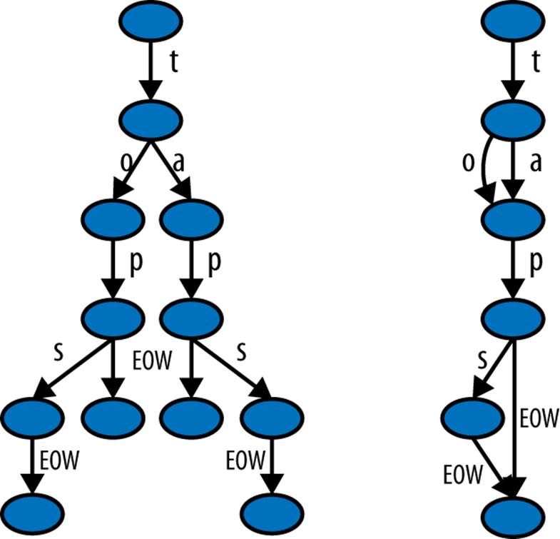
Figure 11-2. Trie and DAWG structures (image by Chkno [CC BY-SA 3.0])

In the following sections, we take a closer look at DAWGs, tries, and their usage.

Directed acyclic word graph (DAWG)

The Directed Acyclic Word Graph (MIT license) attempts to efficiently represent strings that share common prefixes and suffixes.

In Example 11-13 you see the very simple setup for a DAWG. For this implementation, the DAWG cannot be modified after construction; it reads an iterator to construct itself once. The lack of post-construction updates might be a deal breaker for your use case. If so, you might need to look into using a trie instead. The DAWG does support rich queries, including prefix lookups; it also allows persistence and supports storing integer indices as values along with byte and record values.

Example 11-13. Using a DAWG to store the data

import dawg

...

words_dawg = dawg.DAWG(text_example.readers)

As you can see in Example 11-14, for the same set of strings it uses only slightly less RAM than the earlier set example. More similar input text will cause stronger compression.

Example 11-14. Running the DAWG example

$ python text_example_dawg.py

RAM at start 10.3MiB

RAM after creating dawg 968.8MiB, took 63.1s

Summed time to lookup word 0.0049s

Marisa trie

The Marisa trie (dual-licensed LGPL and BSD) is a static trie using Cython bindings to an external library. As it is static, it cannot be modified after construction. Like the DAWG, it supports storing integer indices as values, as well as byte values and record values.

A key can be used to look up a value, and vice versa. All keys sharing the same prefix can be found efficiently. The trie’s contents can be persisted. Example 11-15 illustrates using a Marisa trie to store our sample data.

Example 11-15. Using a Marisa trie to store the data

import marisa_trie

...

words_trie = marisa_trie.Trie(text_example.readers)

In Example 11-16, we can see that there is a marked improvement in RAM storage compared to the DAWG example, but the overall search time is a little slower.

Example 11-16. Running the Marisa trie example

$ python text_example_trie.py

RAM at start 11.0MiB

RAM after creating trie 304.7MiB, took 55.3s

The trie contains 8545076 words

Summed time to lookup word 0.0101s

Datrie

The double-array trie, or datrie (licensed LGPL), uses a prebuilt alphabet to efficiently store keys. This trie can be modified after creation, but only with the same alphabet. It can also find all keys that share the prefix of the provided key, and it supports persistence.

Along with the HAT trie, it offers one of the fastest lookup times.

NOTE

When using the datrie on the Wikipedia example and for past work on DNA representations, it had a pathological build time. It could take minutes or hours to represent DNA strings, compared to other data structures that completed building in seconds.

The datrie needs an alphabet to be presented to the constructor, and only keys using this alphabet are allowed. In our Wikipedia example, this means we need two passes on the raw data. You can see this in Example 11-17. The first pass builds an alphabet of characters into a set, and a second builds the trie. This slower build process allows for faster lookup times.

Example 11-17. Using a double-array trie to store the data

import datrie

...

chars = set()

for word intext_example.readers:

chars.update(word)

trie = datrie.BaseTrie(chars)

...

# having consumed our generator in the first chars pass,

we need to make a new one

readers = text_example.read_words(text_example.SUMMARIZED_FILE) # new generator

for word inreaders:

trie[word] = 0

Sadly, on this example dataset the datrie threw a segmentation fault, so we can’t show you timing information. We chose to include it because in other tests it tended to be slightly faster (but less RAM-efficient) than the following HAT Trie. We have used it with success for DNA searching, so if you have a static problem and it works, you can be confident that it’ll work well. If you have a problem with varying input, however, this might not be a suitable choice.

HAT trie

The HAT trie (licensed MIT) uses a cache-friendly representation to achieve very fast lookups on modern CPUs. It can be modified after construction but otherwise has a very limited API.

For simple use cases it has great performance, but the API limitations (e.g., lack of prefix lookups) might make it less useful for your application. Example 11-18 demonstrates use of the HAT trie on our example dataset.

Example 11-18. Using a HAT trie to store the data

import hat_trie

...

words_trie = hat_trie.Trie()

for word intext_example.readers:

words_trie[word] = 0

As you can see in Example 11-19, the HAT trie offers the fastest lookup times of our new data structures, along with superb RAM usage. The limitations in its API mean that its use is limited, but if you just need fast lookups in a large number of strings, then this might be your solution.

Example 11-19. Running the HAT trie example

$ python text_example_hattrie.py

RAM at start 9.7MiB

RAM after creating trie 254.2MiB, took 44.7s

The trie contains 8545076 words

Summed time to lookup word 0.0051s

Using tries (and DAWGs) in production systems

The trie and DAWG data structures offer good benefits, but you must still benchmark them on your problem rather than blindly adopting them. If you have overlapping sequences in your strings, then it is likely that you’ll see a RAM improvement.

Tries and DAWGs are less well known, but they can provide strong benefits in production systems. We have an impressive success story in Large-Scale Social Media Analysis at Smesh. Jamie Matthews at DapApps (a Python software house based in the UK) also has a story about the use of tries in client systems to enable more efficient and cheaper deployments for customers:

At DabApps, we often try to tackle complex technical architecture problems by dividing them up into small, self-contained components, usually communicating over the network using HTTP. This approach (referred to as a “service-oriented” or “microservice” architecture) has all sorts of benefits, including the possibility of reusing or sharing the functionality of a single component between multiple projects.

One such task that is often a requirement in our consumer-facing client projects is postcode geocoding. This is the task of converting a full UK postcode (for example: “BN1 1AG”) into a latitude and longitude coordinate pair, to enable the application to perform geospatial calculations such as distance measurement.

At its most basic, a geocoding database is a simple mapping between strings, and can conceptually be represented as a dictionary. The dictionary keys are the postcodes, stored in a normalised form (“BN11AG”), and the values are some representation of the coordinates (we used a geohash encoding, but for simplicity imagine a comma-separated pair such as: “50.822921,-0.142871”).

There are approximately 1.7 million postcodes in the UK. Naively loading the full dataset into a Python dictionary, as described above, uses several hundred megabytes of memory. Persisting this data structure to disk using Python’s native pickle format requires an unacceptably large amount of storage space. We knew we could do better.

We experimented with several different in-memory and on-disk storage and serialisation formats, including storing the data externally in databases such as Redis and LevelDB, and compressing the key/values pairs. Eventually, we hit on the idea of using a trie. Tries are extremely efficient at representing large numbers of strings in memory, and the available open-source libraries (we chose “marisa-trie”) make them very simple to use.

The resulting application, including a tiny web API built with the Flask framework, uses only 30MB of memory to represent the entire UK postcode database, and can comfortably handle a high volume of postcode lookup requests. The code is simple; the service is very lightweight and painless to deploy and run on a free hosting platform such as Heroku, with no external requirements or dependencies on databases. Our implementation is open-source, available at https://github.com/j4mie/postcodeserver/.

— Jamie Matthews Technical Director of DabApps.com (UK)

Tips for Using Less RAM

Generally, if you can avoid putting it into RAM, do. Everything you load costs you RAM. You might be able to load just a part of your data, for example using a memory-mapped file; alternatively, you might be able to use generators to load only the part of the data that you need for partial computations rather than loading it all at once.

If you are working with numeric data, then you’ll almost certainly want to switch to using numpy arrays—the package offers many fast algorithms that work directly on the underlying primitive objects. The RAM savings compared to using lists of numbers can be huge, and the time savings can be similarly amazing.

You’ll have noticed in this book that we generally use xrange rather than range, simply because (in Python 2.x) xrange is a generator while range builds an entire list. Building a list of 100,000,000 integers just to iterate the right number of times is excessive—the RAM cost is large and entirely unnecessary. Python 3.x turns range into a generator so you no longer need to make this change.

If you’re working with strings and you’re using Python 2.x, try to stick to str rather than unicode if you want to save RAM. You will probably be better served by simply upgrading to Python 3.3+ if you need lots of Unicode objects throughout your program. If you’re storing a large number of Unicode objects in a static structure, then you probably want to investigate the DAWG and trie structures that we’ve just discussed.

If you’re working with lots of bit strings, investigate numpy and the bitarray package; they both have efficient representations of bits packed into bytes. You might also benefit from looking at Redis, which offers efficient storage of bit patterns.

The PyPy project is experimenting with more efficient representations of homogenous data structures, so long lists of the same primitive type (e.g., integers) might cost much less in PyPy than the equivalent structures in CPython. The Micro Python project will be interesting to anyone working with embedded systems: it is a tiny-memory-footprint implementation of Python that’s aiming for Python 3 compatibility.

It goes (almost!) without saying that you know you have to benchmark when you’re trying to optimize on RAM usage, and that it pays handsomely to have a unit test suite in place before you make algorithmic changes.

Having reviewed ways of compressing strings and storing numbers efficiently, we’ll now look at trading accuracy for storage space.

Probabilistic Data Structures

Probabilistic data structures allow you to make trade-offs in accuracy for immense decreases in memory usage. In addition, the number of operations you can do on them is much more restricted than with a set or a trie. For example, with a single HyperLogLog++ structure using 2.56 KB you can count the number of unique items up to approximately 7,900,000,000 items with 1.625% error.

This means that if we’re trying to count the number of unique license plate numbers for cars, if our HyperLogLog++ counter said there were 654,192,028, we would be confident that the actual number is between 664,822,648 and 643,561,407. Furthermore, if this accuracy isn’t sufficient, you can simply add more memory to the structure and it will perform better. Giving it 40.96 KB of resources will decrease the error from 1.625% to 0.4%. However, storing this data in a set would take 3.925 GB, even assuming no overhead!

On the other hand, the HyperLogLog++ structure would only be able to count a set of license plates and merge with another set. So, for example, we could have one structure for every state, find how many unique license plates are in those states, then merge them all to get a count for the whole country. If we were given a license plate we couldn’t tell you if we’ve seen it before with very good accuracy, and we couldn’t give you a sample of license plates we have already seen.

Probabilistic data structures are fantastic when you have taken the time to understand the problem and need to put something into production that can answer a very small set of questions about a very large set of data. Each different structure has different questions it can answer at different accuracies, so finding the right one is just a matter of understanding your requirements.

In almost all cases, probabilistic data structures work by finding an alternative representation for the data that is more compact and contains the relevant information for answering a certain set of questions. This can be thought of as a type of lossy compression, where we may lose some aspects of the data but we retain the necessary components. Since we are allowing the loss of data that isn’t necessarily relevant for the particular set of questions we care about, this sort of lossy compression can be much more efficient than the lossless compression we looked at before with tries. It is because of this that the choice of which probabilistic data structure you will use is quite important—you want to pick one that retains the right information for your use case!

Before we dive in, it should be made clear that all the “error rates” here are defined in terms of standard deviations. This term comes from describing Gaussian distributions and says how spread out the function is around a center value. When the standard deviation grows, so do the number of values further away from the center point. Error rates for probabilistic data structures are framed this way because all the analyses around them are probabilistic. So, for example, when we say that the HyperLogLog++ algorithm has an error of we mean that 66% of the time the error will be smaller than err, 95% of the time smaller than 2*err, and 99.7% of the time smaller than 3*err.^[32^]

Very Approximate Counting with a 1-byte Morris Counter

We’ll introduce the topic of probabilistic counting with one of the earliest probabilistic counters, the Morris counter (by Robert Morris of the NSA and Bell Labs). Applications include counting millions of objects in a restricted-RAM environment (e.g., on an embedded computer), understanding large data streams, and problems in AI like image and speech recognition.

The Morris counter keeps track of an exponent and models the counted state as (rather than a correct count)—it provides an order of magnitude estimate. This estimate is updated using a probabilistic rule.

We start with the exponent set to 0. If we ask for the value of the counter, we’ll be given pow(2,exponent)=1 (the keen reader will note that this is off by one—we did say this was an approximate counter!). If we ask the counter to increment itself it will generate a random number (using the uniform distribution) and it will test if random(0, 1) <= 1/pow(2,exponent), which will always be true (pow(2,0) == 1). The counter increments, and the exponent is set to 1.

The second time we ask the counter to increment itself it will test if random(0, 1) <= 1/pow(2,1). This will be true 50% of the time. If the test passes, then the exponent is incremented. If not, then the exponent is not incremented for this increment request.

Table 11-1 shows the likelihoods of an increment occurring for each of the first exponents.

Table 11-1. Morris counter details

The maximum we could approximately count where we use a single unsigned byte for the exponent is math.pow(2,255) == 5e76. The error relative to the actual count will be fairly large as the counts increase, but the RAM savings is tremendous as we only use 1 byte rather than the 32 unsigned bytes we’d otherwise have to use. Example 11-20 shows a simple implementation of the Morris counter.

Example 11-20. Simple Morris counter implementation

from random import random

class MorrisCounter(object):

counter = 0

def add(self, *args):

if random() < 1.0 / (2 ** self.counter):

self.counter += 1

def __len__(self):

return 2**self.counter

Using this example implementation, we can see in Example 11-20 that the first request to increment the counter succeeds and the second fails.^[33^]

Example 11-21. Morris counter library example

In [2]: mc = MorrisCounter()

In [3]: print len(mc)

1.0

In [4]: mc.add() # P(1) of doing an add

In [5]: print len(mc)

2.0

In [6]: mc.add() # P(0.5) of doing an add

In [7]: print len(mc) # the add does not occur on this attempt

2.0

In Figure 11-3, the thick black line shows a normal integer incrementing on each iteration. On a 64-bit computer this is an 8-byte integer. The evolution of three 1-byte Morris counters is shown as dotted lines; the y-axis shows their values, which approximately represent the true count for each iteration. Three counters are shown to give you an idea about their different trajectories and the overall trend; the three counters are entirely independent of each other.

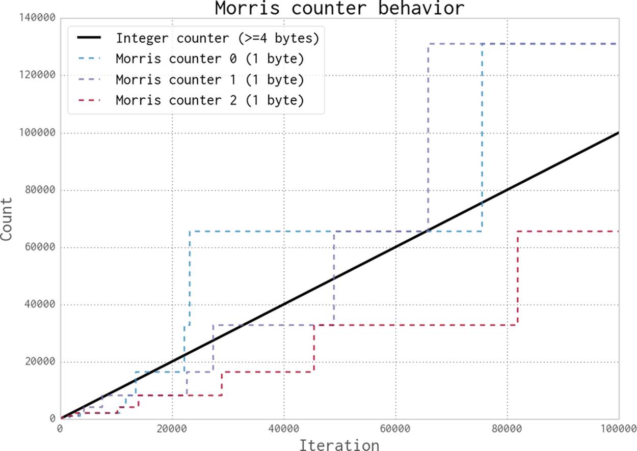
Figure 11-3. Three 1-byte Morris counters vs. an 8-byte integer

This diagram gives you some idea about the error to expect when using a Morris counter. Further details about the error behavior are available online.

K-Minimum Values

In the Morris counter, we lose any sort of information about the items we insert. That is to say, the counter’s internal state is the same whether we do .add("micha") or .add("ian"). This extra information is useful and, if used properly, could help us have our counters only count unique items. In this way, calling .add("micha") thousands of times would only increase the counter once.

To implement this behavior, we will exploit properties of hashing functions (see Hash Functions and Entropy for a more in-depth discussion of hash functions). The main property we would like to take advantage of is the fact that the hash function takes input and uniformly distributes it. For example, let’s assume we have a hash function that takes in a string and outputs a number between 0 and 1. For that function to be uniform means that when we feed it in a string we are equally likely to get a value of 0.5 as a value of 0.2, or any other value. This also means that if we feed it in many string values, we would expect the values to be relatively evenly spaced. Remember, this is a probabilistic argument: the values won’t always be evenly spaced, but if we have many strings and try this experiment many times, they will tend to be evenly spaced.

Suppose we took 100 items and stored the hashes of those values (the hashes being numbers from 0 to 1). Knowing the spacing is even means that instead of saying, “We have 100 items,” we could say “We have a distance of 0.01 between every item.” This is where the K-Minimum Values algorithm^[34^] finally comes in—if we keep the k smallest unique hash values we have seen, we can approximate the overall spacing between hash values and infer what the total number of items is. In Figure 11-4 we can see the state of a K-Minimum Values structure (also called a KMV) as more and more items are added. At first, since we don’t have many hash values, the largest hash we have kept is quite large. As we add more and more, the largest of the k hash values we have kept gets smaller and smaller. Using this method, we can get error rates of .

The larger k is, the more we can account for the hashing function we are using not being completely uniform for our particular input and for unfortunate hash values. An example of unfortunate hash values would be hashing ['A', 'B', 'C'] and getting the values [0.01, 0.02, 0.03]. If we start hashing more and more values, it is less and less probable that they will clump up.

Furthermore, since we are only keeping the smallest unique hash values, the data structure only considers unique inputs. We can see this easily because if we are in a state where we only store the smallest three hashes and currently [0.1, 0.2, 0.3] are the smallest hash values, if we add in something with the hash value of 0.4 our state will not change. Similarly, if we add more items with a hash value of 0.3, our state will also not change. This is a property called idempotence; it means that if we do the same operation, with the same inputs, on this structure multiple times, the state will not be changed. This is in contrast to, for example, an append on a list, which will always change its value. This concept of idempotence carries on to all of the data structures in this section except for the Morris counter.

Example 11-22 shows a very basic K-Minimum Values implementation. Of note is our use of a sortedset, which, like a set, can only contain unique items. This uniqueness gives our KMinValues structure idempotence for free. To see this, follow the code through: when the same item is added more than once, the data property does not change.

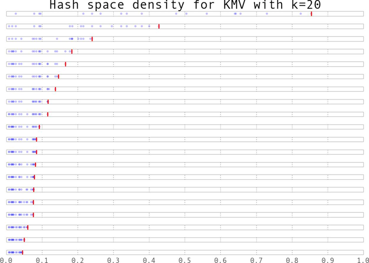
Figure 11-4. The values stores in a KMV structure as more elements are added

Example 11-22. Simple KMinValues implementation

import mmh3

from blist import sortedset

class KMinValues(object):

def __init__(self, num_hashes):

self.num_hashes = num_hashes

self.data = sortedset()

def add(self, item):

item_hash = mmh3.hash(item)

self.data.add(item_hash)

if len(self.data) > self.num_hashes:

self.data.pop()

def __len__(self):

if len(self.data) <= 2:

return 0

return (self.num_hashes - 1) * (2**32-1) / float(self.data[-2] + 2**31 - 1)

Using the KMinValues implementation in the Python package countmemaybe (Example 11-23), we can begin to see the utility of this data structure. This implementation is very similar to the one in Example 11-22, but it fully implements the other set operations, such as union and intersection. Also note that “size” and “cardinality” are used interchangeably (the word “cardinality” is from set theory and is used more in the analysis of probabilistic data structures). Here, we can see that even with a reasonably small value for k, we can store 50,000 items and calculate the cardinality of many set operations with relatively low error.

Example 11-23. countmemaybe KMinValues implementation

>>> from countmemaybe import KMinValues

>>> kmv1 = KMinValues(k=1024)

>>> kmv2 = KMinValues(k=1024)

>>> for i inxrange(0,50000): #

kmv1.add(str(i))

...:

>>> for i inxrange(25000, 75000): #

kmv2.add(str(i))

...:

>>> print len(kmv1)

50416

>>> print len(kmv2)

52439

>>> print kmv1.cardinality_intersection(kmv2)

25900.2862992

>>> print kmv1.cardinality_union(kmv2)

75346.2874158

We put 50,000 elements into kmv1.

kmv2 also gets 50,000 elements, 25,000 of which are the same as those in kmv1.

NOTE

With these sorts of algorithms, the choice of hash function can have a drastic effect on the quality of the estimates. Both of these implementations use mmh3, a Python implementation of mumurhash3 that has nice properties for hashing strings. However, different hash functions could be used if they are more convenient for your particular dataset.

Bloom Filters

Sometimes we need to be able to do other types of set operations, for which we need to introduce new types of probabilistic data structures. Bloom filters^[35^] were created to answer the question of whether we’ve seen an item before.

Bloom filters work by having multiple hash values in order to represent a value as multiple integers. If we later see something with the same set of integers, we can be reasonably confident that it is the same value.

In order to do this in a way that efficiently utilizes available resources, we implicitly encode the integers as the indices of a list. This could be thought of as a list of bool values that are initially set to False. If we are asked to add an object with hash values [10, 4, 7], then we set the tenth, fourth, and seventh indices of the list to True. In the future, if we are asked if we have seen a particular item before, we simply find its hash values and check if all the corresponding spots in the bool list are set to True.

This method gives us no false negatives and a controllable rate of false positives. What this means is that if the Bloom filter says we have not seen an item before, then we can be 100% sure that we haven’t seen the item before. On the other hand, if the Bloom filter states that we have seen an item before, then there is a probability that we actually have not and we are simply seeing an erroneous result. This erroneous result comes from the fact that we will have hash collisions, and sometimes the hash values for two objects will be the same even if the objects themselves are not the same. However, in practice Bloom filters are set to have error rates below 0.5%, so this error can be acceptable.

NOTE

We can simulate having as many hash functions as we want simply by having two hash functions that are independent of each other. This method is called “double hashing.” If we have a hash function that gives us two independent hashes, we can do:

def multi_hash(key, num_hashes):

hash1, hash2 = hashfunction(key)

for i inxrange(num_hashes):

yield (hash1 + i * hash2) % (2^32 - 1)

The modulo ensures that the resulting hash values are 32 bit (we would modulo by 2^64 - 1 for 64-bit hash functions).

The exact length of the bool list and the number of hash values per item we need will be fixed based on the capacity and the error rate we require. With some reasonably simple statistical arguments^[36^] we see that the ideal values are:

That is to say, if we wish to store 50,000 objects (no matter how big the objects themselves are) at a false positive rate of 0.05% (that is to say, 0.05% of the times we say we have seen an object before, we actually have not), it would require 791,015 bits of storage and 11 hash functions.

To further improve our efficiency in terms of memory use, we can use single bits to represent the bool values (a native bool actually takes 4 bits). We can do this easily by using the bitarray module. Example 11-24 shows a simple Bloom filter implementation.

Example 11-24. Simple Bloom filter implemintation

import bitarray

import math

import mmh3

class BloomFilter(object):

def __init__(self, capacity, error=0.005):

"""

Initialize a Bloom filter with given capacity and false positive rate

"""

self.capacity = capacity

self.error = error

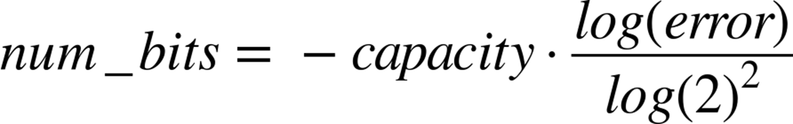
self.num_bits = int(-capacity * math.log(error) / math.log(2)**2) + 1

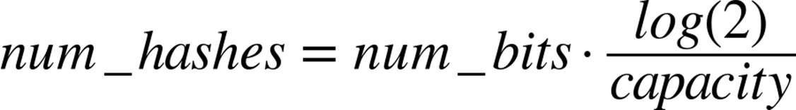
self.num_hashes = int(self.num_bits * math.log(2) / float(capacity)) + 1

self.data = bitarray.bitarray(self.num_bits)

def _indexes(self, key):

h1, h2 = mmh3.hash64(key)

for i inxrange(self.num_hashes):

yield (h1 + i * h2) % self.num_bits

def add(self, key):

for index inself._indexes(key):

self.data[index] = True

def __contains__(self, key):

return all(self.data[index] for index inself._indexes(key))

def __len__(self):

num_bits_on = self.data.count(True)

return -1.0 * self.num_bits *

math.log(1.0 - num_bits_on / float(self.num_bits)) /

float(self.num_hashes)

@staticmethod

def union(bloom_a, bloom_b):

assert bloom_a.capacity == bloom_b.capacity, "Capacities must be equal"

assert bloom_a.error == bloom_b.error, "Error rates must be equal"

bloom_union = BloomFilter(bloom_a.capacity, bloom_a.error)

bloom_union.data = bloom_a.data | bloom_b.data

return bloom_union

What happens if we insert more items than we specified for the capacity of the Bloom filter? At the extreme end, all the items in the bool list will be set to True, in which case we say that we have seen every item. This means that Bloom filters are very sensitive to what their initial capacity was set to, which can be quite aggravating if we are dealing with a set of data whose size is unknown (for example, a stream of data).

One way of dealing with this is to use a variant of Bloom filters called scalable Bloom filters.^[37^] They work by chaining together multiple bloom filters whose error rates vary in a specific way.^[38^] By doing this, we can guarantee an overall error rate and simply add a new Bloom filter when we need more capacity. In order to check if we’ve seen an item before, we simply iterate over all of the sub-Blooms until either we find the object or we exhaust the list. A sample implementation of this structure can be seen in Example 11-25, where we use the previous Bloom filter implementation for the underlying functionality and have a counter to simplify knowing when to add a new Bloom.

Example 11-25. Simple scaling Bloom filter implementation

from bloomfilter import BloomFilter

class ScalingBloomFilter(object):

def __init__(self, capacity, error=0.005,

max_fill=0.8, error_tightening_ratio=0.5):

self.capacity = capacity

self.base_error = error

self.max_fill = max_fill

self.items_until_scale = int(capacity * max_fill)

self.error_tightening_ratio = error_tightening_ratio

self.bloom_filters = []

self.current_bloom = None

self._add_bloom()

def _add_bloom(self):

new_error = self.base_error *

self.error_tightening_ratio ** len(self.bloom_filters)

new_bloom = BloomFilter(self.capacity, new_error)

self.bloom_filters.append(new_bloom)

self.current_bloom = new_bloom

return new_bloom

def add(self, key):

if key inself:

return True

self.current_bloom.add(key)

self.items_until_scale -= 1

if self.items_until_scale == 0:

bloom_size = len(self.current_bloom)

bloom_max_capacity = int(self.current_bloom.capacity * self.max_fill)

# We may have been adding many duplicate values into the Bloom, so

# we need to check if we actually need to scale or if we still have

# space

if bloom_size >= bloom_max_capacity:

self._add_bloom()

self.items_until_scale = bloom_max_capacity

else:

self.items_until_scale = int(bloom_max_capacity - bloom_size)

return False

def __contains__(self, key):

return any(key inbloom for bloom inself.bloom_filters)

def __len__(self):

return sum(len(bloom) for bloom inself.bloom_filters)

Another way of dealing with this is using a method called timing Bloom filters. This variant allows elements to be expired out of the data structure, thus freeing up space for more elements. This is especially nice for dealing with streams, since we can have elements expire after, say, an hour and have the capacity set large enough to deal with the amount of data we see per hour. Using a Bloom filter this way would give us a nice view into what has been happening in the last hour.

Using this data structure will feel much like using a set object. In the following interaction we use the scalable Bloom filter to add several objects, test if we’ve seen them before, and then try to experimentally find the false positive rate:

>>> bloom = BloomFilter(100)

>>> for i inxrange(50):

....: bloom.add(str(i))

....:

>>> "20" inbloom

True

>>> "25" inbloom

True

>>> "51" inbloom

False

>>> num_false_positives = 0

>>> num_true_negatives = 0

>>> # None of the following numbers should be in the Bloom.

>>> # If one is found in the Bloom, it is a false positive.

>>> for i inxrange(51,10000):

....: if str(i) inbloom:

....: num_false_positives += 1

....: else:

....: num_true_negatives += 1

....:

>>> num_false_positives

54

>>> num_true_negatives

9895

>>> false_positive_rate = num_false_positives / float(10000 - 51)

>>> false_positive_rate

0.005427681173987335

>>> bloom.error

0.005

We can also do unions with Bloom filters in order to join multiple sets of items:

>>> bloom_a = BloomFilter(200)

>>> bloom_b = BloomFilter(200)

>>> for i inxrange(50):

...: bloom_a.add(str(i))

...:

>>> for i inxrange(25,75):

...: bloom_b.add(str(i))

...:

>>> bloom = BloomFilter.union(bloom_a, bloom_b)

>>> "51" inbloom_a #

Out[9]: False

>>> "24" inbloom_b #

Out[10]: False

>>> "55" inbloom #

Out[11]: True

>>> "25" inbloom

Out[12]: True

The value of '51' is not in bloom_a.

Similarly, the value of '24' is not in bloom_b.

However, the bloom object contains all the objects in both bloom_a and bloom_b!

One caveat with this is that you can only take the union of two Blooms with the same capacity and error rate. Furthermore, the final Bloom’s used capacity can be as high as the sum of the used capacities of the two Blooms unioned to make it. What this means is that you could start with two Bloom filters that are a little more than half full and, when you union them together, get a new Bloom that is over capacity and not reliable!

LogLog Counter

LogLog-type counters are based on the realization that the individual bits of a hash function can also be considered to be random. That is to say, the probability of the first bit of a hash being 1 is 50%, the probability of the first two bits being 01 is 25%, and the probability of the first three bits being 001 is 12.5%. Knowing these probabilities, and keeping the hash with the most 0s at the beginning (i.e., the least probable hash value), we can come up with an estimate of how many items we’ve seen so far.

A good analogy for this method is flipping coins. Imagine we would like to flip a coin 32 times and get heads every time. The number 32 comes from the fact that we are using 32-bit hash functions. If we flip the coin once and it comes up tails, then we will store the number 0, since our best attempt yielded 0 heads in a row. Since we know the probabilities behind this coin flip, we can also tell you that our longest series was 0 long and you can estimate that we’ve tried this experiment 2^0 = 1 time. If we keep flipping our coin and we’re able to get 10 heads before getting a tail, then we would store the number 10. Using the same logic, you could estimate that we’ve tried the experiment 2^10 = 1024 times. With this system, the highest we could count would be the maximum number of flips we consider (for 32 flips, this is 2^32 = 4,294,967,296).

In order to encode this logic with LogLog-type counters, we take the binary representation of the hash value of our input and see how many 0s there are before we see our first 1. The hash value can be thought of as a series of 32 coin flips, where 0 means a flip for heads and 1 means a flip for tails (i.e., 000010101101 means we flipped four heads before our first tails and 010101101 means we flipped one head before flipping our first tail). This gives us an idea how many tries happened before this hash value was gotten. The mathematics behind this system is almost equivalent to that of the Morris counter, with one major exception: we acquire the “random” values by looking at the actual input instead of using a random number generator. This means that if we keep adding the same value to a LogLog counter its internal state will not change.Example 11-26 shows a simple implementation of a LogLog counter.

Example 11-26. Simple implementation of LogLog register

import mmh3

def trailing_zeros(number):

"""

Returns the index of the first bit set to 1 from the right side of a 32-bit

integer

>>> trailing_zeros(0)

32

>>> trailing_zeros(0b1000)

3

>>> trailing_zeros(0b10000000)

7

"""

if notnumber:

return 32

index = 0

while (number >> index) & 1 == 0:

index += 1

return index

class LogLogRegister(object):

counter = 0

def add(self, item):

item_hash = mmh3.hash(str(item))

return self._add(item_hash)

def _add(self, item_hash):

bit_index = trailing_zeros(item_hash)

if bit_index > self.counter:

self.counter = bit_index

def __len__(self):

return 2**self.counter

The biggest drawback of this method is that we may get a hash value that increases the counter right at the beginning and skews our estimates. This would be similar to flipping 32 tails on the first try. In order to remedy this, we should have many people flipping coins at the same time and combine their results. The law of large numbers tells us that as we add more and more flippers, the total statistics become less affected by anomalous samples from individual flippers. The exact way that we combine the results is the root of the difference between LogLog type methods (classic LogLog, SuperLogLog, HyperLogLog, HyperLogLog++, etc.).

We can accomplish this “multiple flipper” method by taking the first couple of bits of a hash value and using that to designate which of our flippers had that particular result. If we take the first 4 bits of the hash, this means we have 2^4 = 16 flippers. Since we used the first 4 bits for this selection, we only have 28 bits left (corresponding to 28 individual coin flips per coin flipper), meaning each counter can only count up to 2^28 = 268,435,456. In addition, there is a constant (alpha) that depends on the number of flippers there are, which normalizes the estimation.^[39^] All of this together gives us an algorithm with accuracy, where m is the number of registers (or flippers) used.. Example 11-27 shows a simple implementation of the LogLog algorithm.

Example 11-27. Simple implementation of LogLog

from llregister import LLRegister

import mmh3

class LL(object):

def __init__(self, p):

self.p = p

self.num_registers = 2**p

self.registers = [LLRegister() for i inxrange(int(2**p))]

self.alpha = 0.7213 / (1.0 + 1.079 / self.num_registers)

def add(self, item):

item_hash = mmh3.hash(str(item))

register_index = item_hash & (self.num_registers - 1)

register_hash = item_hash >> self.p

self.registers[register_index]._add(register_hash)

def __len__(self):

register_sum = sum(h.counter for h inself.registers)

return self.num_registers * self.alpha *

2 ** (float(register_sum) / self.num_registers)

In addition to this algorithm deduplicating similar items by using the hash value as an indicator, it has a tunable parameter that can be used to dial what sort of accuracy vs. storage compromise you are willing to make.

In the __len__ method, we are averaging the estimates from all of the individual LogLog registers. This, however, is not the most efficient way to combine the data! This is because we may get some unfortunate hash values that make one particular register spike up while the others are still at low values. Because of this, we are only able to achieve an error rate of , where m is the number of registers used.

SuperLogLog^[40^] was devised as a fix to this problem. With this algorithm, only the lowest 70% of the registers were used for the size estimate, and their value was limited by a maximum value given by a restriction rule. This addition decreased the error rate to . This is counterintuitive, since we got a better estimate by disregarding information!

Finally, HyperLogLog^[41^] came out in 2007 and gave us further accuracy gains. It did so simply by changing the method of averaging the individual registers: instead of simply averaging, we use a spherical averaging scheme that also has special considerations for different edge cases the structure could be in. This brings us to the current best error rate of . In addition, this formulation removes a sorting operation that is necessary with SuperLogLog. This can greatly speed up the performance of the data structure when you are trying to insert items at a high volume.Example 11-28 shows a simple implementation of HyperLogLog.

Example 11-28. Simple implementation of HyperLogLog

from ll import LL

import math

class HyperLogLog(LL):

def __len__(self):

indicator = sum(2**-m.counter for m inself.registers)

E = self.alpha * (self.num_registers**2) / float(indicator)

if E <= 5.0 / 2.0 * self.num_registers:

V = sum(1 for m inself.registers if m.counter == 0)

if V != 0:

Estar = self.num_registers *

math.log(self.num_registers / (1.0 * V), 2)

else:

Estar = E

else:

if E <= 2**32 / 30.0:

Estar = E

else:

Estar = -2**32 * math.log(1 - E / 2**32, 2)

return Estar

if __name__ == "__main__":

import mmh3

hll = HyperLogLog(8)

for i inxrange(100000):

hll.add(mmh3.hash(str(i)))

print len(hll)

The only further increase in accuracy was given by the HyperLogLog++ algorithm, which increased the accuracy of the data structure while it is relatively empty. When more items are inserted, this scheme reverts to standard HyperLogLog. This is actually quite useful, since the statistics of the LogLog-type counters require a lot of data to be accurate—having a scheme for allowing better accuracy with fewer number items greatly improves the usability of this method. This extra accuracy is achieved by having a smaller but more accurate HyperLogLog structure that can be later converted into the larger structure that was originally requested. Also, there are some imperially derived constants that are used in the size estimates that remove biases.

Real-World Example

For a better understanding of the data structures, we first created a dataset with many unique keys, and then one with duplicate entries. Figures 11-5 and 11-6 show the results when we feed these keys into the data structures we’ve just looked at and periodically query, “How many unique entries have there been?” We can see that the data structures that contain more stateful variables (such as HyperLogLog and KMinValues) do better, since they more robustly handle bad statistics. On the other hand, the Morris counter and the single LogLog register can quickly have very high error rates if one unfortunate random number or hash value occurs. For most of the algorithms, however, we know that the number of stateful variables is directly correlated with the error guarantees, so this makes sense.

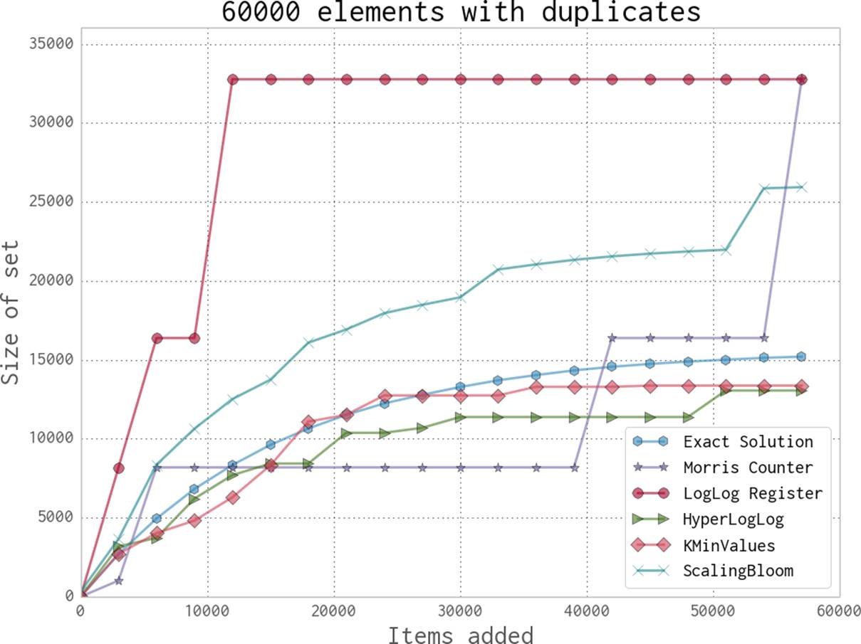
Figure 11-5. Comparison between various probabilistic data structures for repeating data

Looking just at the probabilistic data structures that have the best performance (and really, the ones you will probably use), we can summarize their utility and their approximate memory usage (see Table 11-2). We can see a huge change in memory usage depending on the questions we care to ask. This simply highlights the fact that when using a probabilistic data structure, you must first consider what questions you really need to answer about the dataset before proceeding. Also note that only the Bloom filter’s size depends on the number of elements. The HyperLogLog and KMinValues’s sizes are only dependent on the error rate.

As another, more realistic test, we chose to use a dataset derived from the text of Wikipedia. We ran a very simple script in order to extract all single-word tokens with five or more characters from all articles and store them in a newline-separated file. The question then was, “How many unique tokens are there?” The results can be seen in Table 11-3. In addition, we attempted to answer the same question using the datrie from Datrie (this trie was chosen as opposed to the others because it offers good compression while still being robust enough to deal with the entire dataset).

Table 11-2. Comparison of major probabilistic data structures

The major takeaway from this experiment is that if you are able to specialize your code, you can get amazing speed and memory gains. This has been true throughout the entire book: when we specialized our code in Selective Optimizations: Finding What Needs to Be Fixed, we were similarly able to get speed increases.

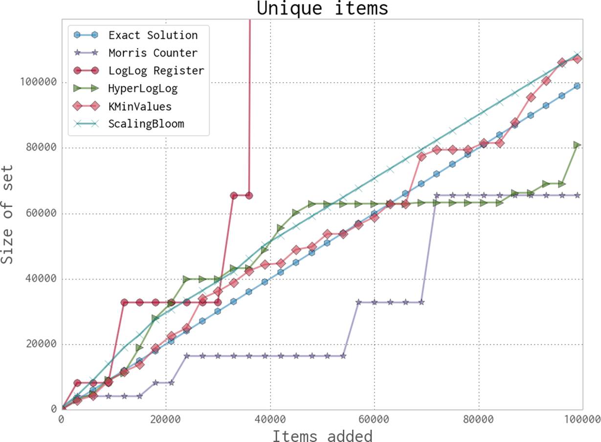
Figure 11-6. Comparison between various probabilistic data structures for unique data

Probabilistic data structures are an algorithmic way of specializing your code. We store only the data we need in order to answer specific questions with given error bounds. By only having to deal with a subset of the information given, not only can we make the memory footprint much smaller, but we can also perform most operations over the structure faster (as can be seen with the insertion time into the datrie in Table 11-3 being larger than any of the probabilistic data structures).

Table 11-3. Size estimates for the number of unique words in Wikipedia

As a result, whether or not you use probabilistic data structures, you should always keep in mind what questions you are going to be asking of your data and how you can most effectively store that data in order to ask those specialized questions. This may come down to using one particular type of list over another, using one particular type of database index over another, or maybe even using a probabilistic data structure to throw out all but the relevant data!