High Performance Python (2014)
Chapter 2. Profiling to Find Bottlenecks
QUESTIONS YOU’LL BE ABLE TO ANSWER AFTER THIS CHAPTER
§ How can I identify speed and RAM bottlenecks in my code?
§ How do I profile CPU and memory usage?
§ What depth of profiling should I use?
§ How can I profile a long-running application?
§ What’s happening under the hood with CPython?
§ How do I keep my code correct while tuning performance?
Profiling lets us find bottlenecks so we can do the least amount of work to get the biggest practical performance gain. While we’d like to get huge gains in speed and reductions in resource usage with little work, practically you’ll aim for your code to run “fast enough” and “lean enough” to fit your needs. Profiling will let you make the most pragmatic decisions for the least overall effort.
Any measurable resource can be profiled (not just the CPU!). In this chapter we look at both CPU time and memory usage. You could apply similar techniques to measure network bandwidth and disk I/O too.
If a program is running too slowly or using too much RAM, then you’ll want to fix whichever parts of your code are responsible. You could, of course, skip profiling and fix what you believe might be the problem—but be wary, as you’ll often end up “fixing” the wrong thing. Rather than using your intuition, it is far more sensible to first profile, having defined a hypothesis, before making changes to the structure of your code.
Sometimes it’s good to be lazy. By profiling first, you can quickly identify the bottlenecks that need to be solved, and then you can solve just enough of these to achieve the performance you need. If you avoid profiling and jump to optimization, then it is quite likely that you’ll do more work in the long run. Always be driven by the results of profiling.
Profiling Efficiently
The first aim of profiling is to test a representative system to identify what’s slow (or using too much RAM, or causing too much disk I/O or network I/O). Profiling typically adds an overhead (10x to 100x slowdowns can be typical), and you still want your code to be used as similarly to in a real-world situation as possible. Extract a test case and isolate the piece of the system that you need to test. Preferably, it’ll have been written to be in its own set of modules already.
The basic techniques that are introduced first in this chapter include the %timeit magic in IPython, time.time(), and a timing decorator. You can use these techniques to understand the behavior of statements and functions.
Then we will cover cProfile (Using the cProfile Module), showing you how to use this built-in tool to understand which functions in your code take the longest to run. This will give you a high-level view of the problem so you can direct your attention to the critical functions.
Next, we’ll look at line_profiler (Using line_profiler for Line-by-Line Measurements), which will profile your chosen functions on a line-by-line basis. The result will include a count of the number of times each line is called and the percentage of time spent on each line. This is exactly the information you need to understand what’s running slowly and why.
Armed with the results of line_profiler, you’ll have the information you need to move on to using a compiler (Chapter 7).
In Chapter 6 (Example 6-8), you’ll learn how to use perf stat to understand the number of instructions that are ultimately executed on a CPU and how efficiently the CPU’s caches are utilized. This allows for advanced-level tuning of matrix operations. You should take a look at that example when you’re done with this chapter.
After line_profiler we show you heapy (Inspecting Objects on the Heap with heapy), which can track all of the objects inside Python’s memory—this is great for hunting down strange memory leaks. If you’re working with long-running systems, then dowser (Using dowser for Live Graphing of Instantiated Variables) will interest you; it allows you to introspect live objects in a long-running process via a web browser interface.
To help you understand why your RAM usage is high, we’ll show you memory_profiler (Using memory_profiler to Diagnose Memory Usage). It is particularly useful for tracking RAM usage over time on a labeled chart, so you can explain to colleagues why certain functions use more RAM than expected.
NOTE
Whatever approach you take to profiling your code, you must remember to have adequate unit test coverage in your code. Unit tests help you to avoid silly mistakes and help to keep your results reproducible. Avoid them at your peril.
Always profile your code before compiling or rewriting your algorithms. You need evidence to determine the most efficient ways to make your code run faster.
Finally, we’ll give you an introduction to the Python bytecode inside CPython (Using the dis Module to Examine CPython Bytecode), so you can understand what’s happening “under the hood.” In particular, having an understanding of how Python’s stack-based virtual machine operates will help you to understand why certain coding styles run more slowly than others.
Before the end of the chapter, we’ll review how to integrate unit tests while profiling (Unit Testing During Optimization to Maintain Correctness), to preserve the correctness of your code while you make it run more efficiently.
We’ll finish with a discussion of profiling strategies (Strategies to Profile Your Code Successfully), so you can reliably profile your code and gather the correct data to test your hypotheses. Here you’ll learn about how dynamic CPU frequency scaling and features like TurboBoost can skew your profiling results and how they can be disabled.
To walk through all of these steps, we need an easy-to-analyze function. The next section introduces the Julia set. It is a CPU-bound function that’s a little hungry for RAM; it also exhibits nonlinear behavior (so we can’t easily predict the outcomes), which means we need to profile it at runtime rather than analyzing it offline.
Introducing the Julia Set
The Julia set is an interesting CPU-bound problem for us to begin with. It is a fractal sequence that generates a complex output image, named after Gaston Julia.
The code that follows is a little longer than a version you might write yourself. It has a CPU-bound component and a very explicit set of inputs. This configuration allows us to profile both the CPU usage and the RAM usage so we can understand which parts of our code are consuming two of our scarce computing resources. This implementation is deliberately suboptimal, so we can identify memory-consuming operations and slow statements. Later in this chapter we’ll fix a slow logic statement and a memory-consuming statement, and in Chapter 7 we’ll significantly speed up the overall execution time of this function.
We will analyze a block of code that produces both a false grayscale plot (Figure 2-1) and a pure grayscale variant of the Julia set (Figure 2-3), at the complex point c=-0.62772-0.42193j. A Julia set is produced by calculating each pixel in isolation; this is an “embarrassingly parallel problem” as no data is shared between points.

Figure 2-1. Julia set plot with a false grayscale to highlight detail
If we chose a different c, then we’d get a different image. The location we have chosen has regions that are quick to calculate and others that are slow to calculate; this is useful for our analysis.
The problem is interesting because we calculate each pixel by applying a loop that could be applied an indeterminate number of times. On each iteration we test to see if this coordinate’s value escapes toward infinity, or if it seems to be held by an attractor. Coordinates that cause few iterations are colored darkly in Figure 2-1, and those that cause a high number of iterations are colored white. White regions are more complex to calculate and so take longer to generate.
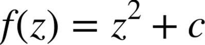
We define a set of z-coordinates that we’ll test. The function that we calculate squares the complex number z and adds c:
We iterate on this function while testing to see if the escape condition holds using abs. If the escape function is False, then we break out of the loop and record the number of iterations we performed at this coordinate. If the escape function is never False, then we stop after maxiteriterations. We will later turn this z’s result into a colored pixel representing this complex location.
In pseudocode, it might look like:
for z incoordinates:
for iteration inrange(maxiter): # limited iterations per point
if abs(z) < 2.0: # has the escape condition been broken?
z = z*z + c
else:
break
# store the iteration count for each z and draw later
To explain this function, let’s try two coordinates.
First, we’ll use the coordinate that we draw in the top-left corner of the plot at -1.8-1.8j. We must test abs(z) < 2 before we can try the update rule:
z = -1.8-1.8j
print abs(z)
2.54558441227
We can see that for the top-left coordinate the abs(z) test will be False on the zeroth iteration, so we do not perform the update rule. The output value for this coordinate is 0.
Now let’s jump to the center of the plot at z = 0 + 0j and try a few iterations:
c = -0.62772-0.42193j
z = 0+0j
for n inrange(9):
z = z*z + c
print "{}: z={:33}, abs(z)={:0.2f}, c={}".format(n, z, abs(z), c)
0: z= (-0.62772-0.42193j), abs(z)=0.76, c=(-0.62772-0.42193j)
1: z= (-0.4117125265+0.1077777992j), abs(z)=0.43, c=(-0.62772-0.42193j)
2: z=(-0.469828849523-0.510676940018j), abs(z)=0.69, c=(-0.62772-0.42193j)
3: z=(-0.667771789222+0.057931518414j), abs(z)=0.67, c=(-0.62772-0.42193j)
4: z=(-0.185156898345-0.499300067407j), abs(z)=0.53, c=(-0.62772-0.42193j)
5: z=(-0.842737480308-0.237032296351j), abs(z)=0.88, c=(-0.62772-0.42193j)
6: z=(0.026302151203-0.0224179996428j), abs(z)=0.03, c=(-0.62772-0.42193j)
7: z= (-0.62753076355-0.423109283233j), abs(z)=0.76, c=(-0.62772-0.42193j)
8: z=(-0.412946606356+0.109098183144j), abs(z)=0.43, c=(-0.62772-0.42193j)
We can see that each update to z for these first iterations leaves it with a value where abs(z) < 2 is True. For this coordinate we can iterate 300 times, and still the test will be True. We cannot tell how many iterations we must perform before the condition becomes False, and this may be an infinite sequence. The maximum iteration (maxiter) break clause will stop us iterating potentially forever.
In Figure 2-2 we see the first 50 iterations of the preceding sequence. For 0+0j (the solid line with circle markers) the sequence appears to repeat every eighth iteration, but each sequence of seven calculations has a minor deviation from the previous sequence—we can’t tell if this point will iterate forever within the boundary condition, or for a long time, or maybe for just a few more iterations. The dashed cutoff line shows the boundary at +2.
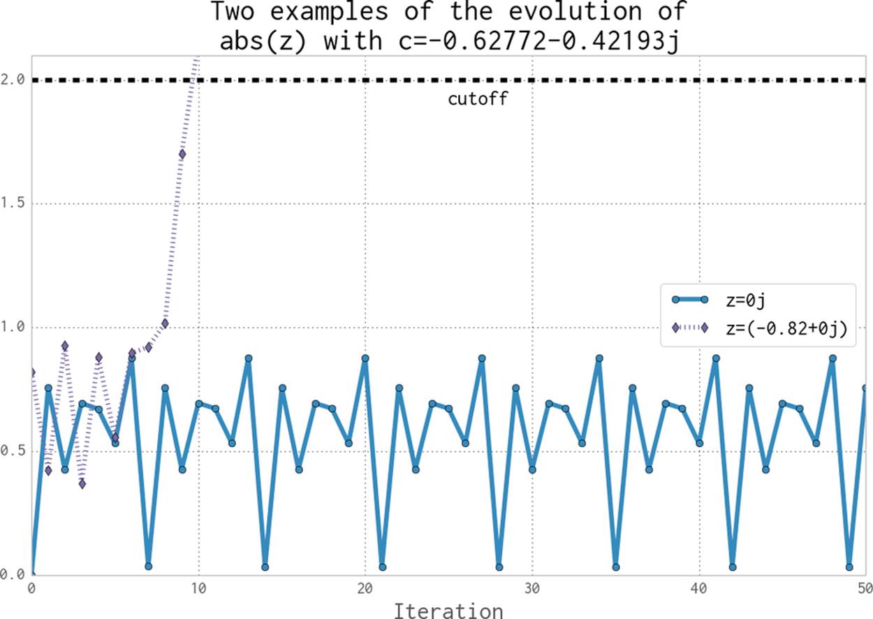
Figure 2-2. Two coordinate examples evolving for the Julia set
For -0.82+0j (the dashed line with diamond markers), we can see that after the ninth update the absolute result has exceeded the +2 cutoff, so we stop updating this value.
Calculating the Full Julia Set
In this section we break down the code that generates the Julia set. We’ll analyze it in various ways throughout this chapter. As shown in Example 2-1, at the start of our module we import the time module for our first profiling approach and define some coordinate constants.
Example 2-1. Defining global constants for the coordinate space
"""Julia set generator without optional PIL-based image drawing"""
import time
# area of complex space to investigate
x1, x2, y1, y2 = -1.8, 1.8, -1.8, 1.8
c_real, c_imag = -0.62772, -.42193
To generate the plot, we create two lists of input data. The first is zs (complex z-coordinates), and the second is cs (a complex initial condition). Neither list varies, and we could optimize cs to a single c value as a constant. The rationale for building two input lists is so that we have some reasonable-looking data to profile when we profile RAM usage later in this chapter.
To build the zs and cs lists, we need to know the coordinates for each z. In Example 2-2 we build up these coordinates using xcoord and ycoord and a specified x_step and y_step. The somewhat verbose nature of this setup is useful when porting the code to other tools (e.g., to numpy) and to other Python environments, as it helps to have everything very clearly defined for debugging.
Example 2-2. Establishing the coordinate lists as inputs to our calculation function
def calc_pure_python(desired_width, max_iterations):
"""Create a list of complex coordinates (zs) and complex
parameters (cs), build Julia set, and display"""
x_step = (float(x2 - x1) / float(desired_width))
y_step = (float(y1 - y2) / float(desired_width))
x = []
y = []
ycoord = y2
while ycoord > y1:
y.append(ycoord)
ycoord += y_step
xcoord = x1
while xcoord < x2:
x.append(xcoord)
xcoord += x_step
# Build a list of coordinates and the initial condition for each cell.
# Note that our initial condition is a constant and could easily be removed;
# we use it to simulate a real-world scenario with several inputs to
# our function.
zs = []
cs = []
for ycoord iny:
for xcoord inx:
zs.append(complex(xcoord, ycoord))
cs.append(complex(c_real, c_imag))
print "Length of x:", len(x)
print "Total elements:", len(zs)
start_time = time.time()
output = calculate_z_serial_purepython(max_iterations, zs, cs)
end_time = time.time()
secs = end_time - start_time
print calculate_z_serial_purepython.func_name + " took", secs, "seconds"
# This sum is expected for a 1000^2 grid with 300 iterations.
# It catches minor errors we might introduce when we're
# working on a fixed set of inputs.
assert sum(output) == 33219980
Having built the zs and cs lists, we output some information about the size of the lists and calculate the output list via calculate_z_serial_purepython. Finally, we sum the contents of output and assert that it matches the expected output value. Ian uses it here to confirm that no errors creep into the book.
As the code is deterministic, we can verify that the function works as we expect by summing all the calculated values. This is useful as a sanity check—when we make changes to numerical code it is very sensible to check that we haven’t broken the algorithm. Ideally we would use unit tests and we’d test more than one configuration of the problem.
Next, in Example 2-3, we define the calculate_z_serial_purepython function, which expands on the algorithm we discussed earlier. Notably, we also define an output list at the start that has the same length as the input zs and cs lists. You may also wonder why we’re using rangerather than xrange–this is so, in Using memory_profiler to Diagnose Memory Usage, we can show how wasteful range can be!
Example 2-3. Our CPU-bound calculation function
def calculate_z_serial_purepython(maxiter, zs, cs):
"""Calculate output list using Julia update rule"""
output = [0] * len(zs)
for i inrange(len(zs)):
n = 0
z = zs[i]
c = cs[i]
while abs(z) < 2 andn < maxiter:
z = z * z + c
n += 1
output[i] = n
return output
Now we call the calculation routine in Example 2-4. By wrapping it in a __main__ check, we can safely import the module without starting the calculations for some of the profiling methods. Note that here we’re not showing the method used to plot the output.
Example 2-4. main for our code
if __name__ == "__main__":
# Calculate the Julia set using a pure Python solution with
# reasonable defaults for a laptop
calc_pure_python(desired_width=1000, max_iterations=300)
Once we run the code, we see some output about the complexity of the problem:
# running the above produces:
Length of x: 1000
Total elements: 1000000
calculate_z_serial_purepython took 12.3479790688 seconds
In the false-grayscale plot (Figure 2-1), the high-contrast color changes gave us an idea of where the cost of the function was slow-changing or fast-changing. Here, in Figure 2-3, we have a linear color map: black is quick to calculate and white is expensive to calculate.
By showing two representations of the same data, we can see that lots of detail is lost in the linear mapping. Sometimes it can be useful to have various representations in mind when investigating the cost of a function.

Figure 2-3. Julia plot example using a pure grayscale
Simple Approaches to Timing—print and a Decorator
After Example 2-4, we saw the output generated by several print statements in our code. On Ian’s laptop this code takes approximately 12 seconds to run using CPython 2.7. It is useful to note that there is always some variation in execution time. You must observe the normal variation when you’re timing your code, or you might incorrectly attribute an improvement in your code simply to a random variation in execution time.
Your computer will be performing other tasks while running your code, such as accessing the network, disk, or RAM, and these factors can cause variations in the execution time of your program.
Ian’s laptop is a Dell E6420 with an Intel Core I7-2720QM CPU (2.20 GHz, 6 MB cache, Quad Core) and 8 GB of RAM running Ubuntu 13.10.
In calc_pure_python (Example 2-2), we can see several print statements. This is the simplest way to measure the execution time of a piece of code inside a function. It is a very basic approach, but despite being quick and dirty it can be very useful when you’re first looking at a piece of code.
Using print statements is commonplace when debugging and profiling code. It quickly becomes unmanageable, but is useful for short investigations. Try to tidy them up when you’re done with them, or they will clutter your stdout.
A slightly cleaner approach is to use a decorator—here, we add one line of code above the function that we care about. Our decorator can be very simple and just replicate the effect of the print statements. Later, we can make it more advanced.
In Example 2-5 we define a new function, timefn, which takes a function as an argument: the inner function, measure_time, takes *args (a variable number of positional arguments) and **kwargs (a variable number of key/value arguments) and passes them through to fn for execution. Around the execution of fn we capture time.time() and then print the result along with fn.func_name. The overhead of using this decorator is small, but if you’re calling fn millions of times the overhead might become noticeable. We use @wraps(fn) to expose the function name and docstring to the caller of the decorated function (otherwise, we would see the function name and docstring for the decorator, not the function it decorates).
Example 2-5. Defining a decorator to automate timing measurements
from functools import wraps
def timefn(fn):
@wraps(fn)
def measure_time(*args, **kwargs):
t1 = time.time()
result = fn(*args, **kwargs)
t2 = time.time()
print ("@timefn:" + fn.func_name + " took " + str(t2 - t1) + " seconds")
return result
return measure_time
@timefn
def calculate_z_serial_purepython(maxiter, zs, cs):
...
When we run this version (we keep the print statements from before), we can see that the execution time in the decorated version is very slightly quicker than the call from calc_pure_python. This is due to the overhead of calling a function (the difference is very tiny):
Length of x: 1000
Total elements: 1000000
@timefn:calculate_z_serial_purepython took 12.2218790054 seconds
calculate_z_serial_purepython took 12.2219250043 seconds
NOTE
The addition of profiling information will inevitably slow your code down—some profiling options are very informative and induce a heavy speed penalty. The trade-off between profiling detail and speed will be something you have to consider.
We can use the timeit module as another way to get a coarse measurement of the execution speed of our CPU-bound function. More typically, you would use this when timing different types of simple expressions as you experiment with ways to solve a problem.
WARNING
Note that the timeit module temporarily disables the garbage collector. This might impact the speed you’ll see with real-world operations if the garbage collector would normally be invoked by your operations. See the Python documentation for help on this.
From the command line you can run timeit using:
$ python -m timeit -n 5 -r 5 -s "import julia1"
"julia1.calc_pure_python(desired_width=1000,
max_iterations=300)"
Note that you have to import the module as a setup step using -s, as calc_pure_python is inside that module. timeit has some sensible defaults for short sections of code, but for longer-running functions it can be sensible to specify the number of loops, whose results are averaged for each test (-n 5), and the number of repetitions (-r 5). The best result of all the repetitions is given as the answer.
By default, if we run timeit on this function without specifying -n and -r it runs 10 loops with 5 repetitions, and this takes 6 minutes to complete. Overriding the defaults can make sense if you want to get your results a little faster.
We’re only interested in the best-case results, as the average and worst case are probably a result of interference by other processes. Choosing the best of five repetitions of five averaged results should give us a fairly stable result:
5 loops, best of 5: 13.1 sec per loop
Try running the benchmark several times to check if you get varying results—you may need more repetitions to settle on a stable fastest-result time. There is no “correct” configuration, so if you see a wide variation in your timing results, do more repetitions until your final result is stable.
Our results show that the overall cost of calling calc_pure_python is 13.1 seconds (as the best case), while single calls to calculate_z_serial_purepython take 12.2 seconds as measured by the @timefn decorator. The difference is mainly the time taken to create the zs and cslists.
Inside IPython, we can use the magic %timeit in the same way. If you are developing your code interactively in IPython and the functions are in the local namespace (probably because you’re using %run), then you can use:
%timeit calc_pure_python(desired_width=1000, max_iterations=300)
It is worth considering the variation in load that you get on a normal computer. Many background tasks are running (e.g., Dropbox, backups) that could impact the CPU and disk resources at random. Scripts in web pages can also cause unpredictable resource usage. Figure 2-4 shows the single CPU being used at 100% for some of the timing steps we just performed; the other cores on this machine are each lightly working on other tasks.
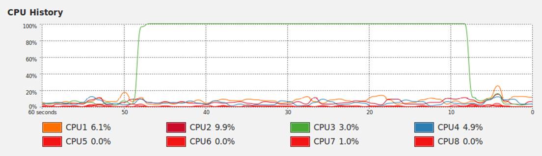
Figure 2-4. System Monitor on Ubuntu showing variation in background CPU usage while we time our function
Occasionally the System Monitor shows spikes of activity on this machine. It is sensible to watch your System Monitor to check that nothing else is interfering with your critical resources (CPU, disk, network).
Simple Timing Using the Unix time Command
We can step outside of Python for a moment to use a standard system utility on Unix-like systems. The following will record various views on the execution time of your program, and it won’t care about the internal structure of your code:
$ /usr/bin/time -p python julia1_nopil.py
Length of x: 1000
Total elements: 1000000
calculate_z_serial_purepython took 12.7298331261 seconds
real 13.46
user 13.40
sys 0.04
Note that we specifically use /usr/bin/time rather than time so we get the system’s time and not the simpler (and less useful) version built into our shell. If you try time --verbose and you get an error, you’re probably looking at the shell’s built-in time command and not the system command.
Using the -p portability flag, we get three results:
§ real records the wall clock or elapsed time.
§ user records the amount of time the CPU spent on your task outside of kernel functions.
§ sys records the time spent in kernel-level functions.
By adding user and sys, you get a sense of how much time was spent in the CPU. The difference between this and real might tell you about the amount of time spent waiting for I/O; it might also suggest that your system is busy running other tasks that are distorting your measurements.
time is useful because it isn’t specific to Python. It includes the time taken to start the python executable, which might be significant if you start lots of fresh processes (rather than having a long-running single process). If you often have short-running scripts where the startup time is a significant part of the overall runtime, then time can be a more useful measure.
We can add the --verbose flag to get even more output:
$ /usr/bin/time --verbose python julia1_nopil.py
Length of x: 1000
Total elements: 1000000
calculate_z_serial_purepython took 12.3145110607 seconds
Command being timed: "python julia1_nopil.py"
User time (seconds): 13.46
System time (seconds): 0.05
Percent of CPU this job got: 99%
Elapsed (wall clock) time (h:mm:ss or m:ss): 0:13.53
Average shared text size (kbytes): 0
Average unshared data size (kbytes): 0
Average stack size (kbytes): 0
Average total size (kbytes): 0
Maximum resident set size (kbytes): 131952
Average resident set size (kbytes): 0
Major (requiring I/O) page faults: 0
Minor (reclaiming a frame) page faults: 58974
Voluntary context switches: 3
Involuntary context switches: 26
Swaps: 0
File system inputs: 0
File system outputs: 1968
Socket messages sent: 0
Socket messages received: 0
Signals delivered: 0
Page size (bytes): 4096
Exit status: 0
Probably the most useful indicator here is Major (requiring I/O) page faults, as this indicates whether the operating system is having to load pages of data from the disk because the data no longer resides in RAM. This will cause a speed penalty.
In our example the code and data requirements are small, so no page faults occur. If you have a memory-bound process, or several programs that use variable and large amounts of RAM, you might find that this gives you a clue as to which program is being slowed down by disk accesses at the operating system level because parts of it have been swapped out of RAM to disk.
Using the cProfile Module
cProfile is a built-in profiling tool in the standard library. It hooks into the virtual machine in CPython to measure the time taken to run every function that it sees. This introduces a greater overhead, but you get correspondingly more information. Sometimes the additional information can lead to surprising insights into your code.
cProfile is one of three profilers in the standard library; the others are hotshot and profile. hotshot is experimental code, and profile is the original pure-Python profiler. cProfile has the same interface as profile, is supported, and is the default profiling tool. If you’re curious about the history of these libraries, see Armin Rigo’s 2005 request to include cProfile in the standard library.
A good practice when profiling is to generate a hypothesis about the speed of parts of your code before you profile it. Ian likes to print out the code snippet in question and annotate it. Forming a hypothesis ahead of time means you can measure how wrong you are (and you will be!) and improve your intuition about certain coding styles.
WARNING
You should never avoid profiling in favor of a gut instinct (we warn you—you will get it wrong!). It is definitely worth forming a hypothesis ahead of profiling to help you learn to spot possible slow choices in your code, and you should always back up your choices with evidence.
Always be driven by results that you have measured, and always start with some quick-and-dirty profiling to make sure you’re addressing the right area. There’s nothing more humbling than cleverly optimizing a section of code only to realize (hours or days later) that you missed the slowest part of the process and haven’t really addressed the underlying problem at all.
So what’s our hypothesis? We know that calculate_z_serial_purepython is likely to be the slowest part of the code. In that function, we do a lot of dereferencing and make many calls to basic arithmetic operators and the abs function. These will probably show up as consumers of CPU resources.
Here, we’ll use the cProfile module to run a variant of the code. The output is spartan but helps us figure out where to analyze further.
The -s cumulative flag tells cProfile to sort by cumulative time spent inside each function; this gives us a view into the slowest parts of a section of code. The cProfile output is written to screen directly after our usual print results:
$ python -m cProfile -s cumulative julia1_nopil.py
...
36221992 function calls in 19.664 seconds
Ordered by: cumulative time
ncalls tottime percall cumtime percall filename:lineno(function)
1 0.034 0.034 19.664 19.664 julia1_nopil.py:1(<module>)
1 0.843 0.843 19.630 19.630 julia1_nopil.py:23
(calc_pure_python)
1 14.121 14.121 18.627 18.627 julia1_nopil.py:9
(calculate_z_serial_purepython)
34219980 4.487 0.000 4.487 0.000 {abs}
2002000 0.150 0.000 0.150 0.000 {method 'append' of 'list' objects}
1 0.019 0.019 0.019 0.019 {range}
1 0.010 0.010 0.010 0.010 {sum}
2 0.000 0.000 0.000 0.000 {time.time}
4 0.000 0.000 0.000 0.000 {len}
1 0.000 0.000 0.000 0.000 {method 'disable' of
'_lsprof.Profiler' objects}
Sorting by cumulative time gives us an idea about where the majority of execution time is spent. This result shows us that 36,221,992 function calls occurred in just over 19 seconds (this time includes the overhead of using cProfile). Previously our code took around 13 seconds to execute—we’ve just added a 5-second penalty by measuring how long each function takes to execute.
We can see that the entry point to the code julia1_cprofile.py on line 1 takes a total of 19 seconds. This is just the __main__ call to calc_pure_python. ncalls is 1, indicating that this line is only executed once.
Inside calc_pure_python, the call to calculate_z_serial_purepython consumes 18.6 seconds. Both functions are only called once. We can derive that approximately 1 second is spent on lines of code inside calc_pure_python, separate to calling the CPU-intensivecalculate_z_serial_purepython function. We can’t derive which lines, however, take the time inside the function using cProfile.
Inside calculate_z_serial_purepython, the time spent on lines of code (without calling other functions) is 14.1 seconds. This function makes 34,219,980 calls to abs, which take a total of 4.4 seconds, along with some other calls that do not cost much time.
What about the {abs} call? This line is measuring the individual calls to the abs function inside calculate_z_serial_purepython. While the per-call cost is negligible (it is recorded as 0.000 seconds), the total time for 34,219,980 calls is 4.4 seconds. We couldn’t predict in advance exactly how many calls would be made to abs, as the Julia function has unpredictable dynamics (that’s why it is so interesting to look at).
At best we could have said that it will be called a minimum of 1,000,000 times, as we’re calculating 1000*1000 pixels. At most it will be called 300,000,000 times, as we calculate 1,000,000 pixels with a maximum of 300 iterations. So, 34 million calls is roughly 10% of the worst case.
If we look at the original grayscale image (Figure 2-3) and, in our mind’s eye, squash the white parts together and into a corner, we can estimate that the expensive white region accounts for roughly 10% of the rest of the image.
The next line in the profiled output, {method 'append' of 'list' objects}, details the creation of 2,002,000 list items.
TIP
Why 2,002,000 items? Before you read on, think about how many list items are being constructed.
This creation of the 2,002,000 items is occurring in calc_pure_python during the setup phase.
The zs and cs lists will be 1000*1000 items each, and these are built from a list of 1,000 x- and 1,000 y-coordinates. In total, this is 2,002,000 calls to append.
It is important to note that this cProfile output is not ordered by parent functions; it is summarizing the expense of all functions in the executed block of code. Figuring out what is happening on a line-by-line basis is very hard with cProfile, as we only get profile information for the function calls themselves, not each line within the functions.
Inside calculate_z_serial_purepython we can now account for {abs} and {range}, and in total these two functions cost approximately 4.5 seconds. We know that calculate_z_serial_purepython costs 18.6 seconds in total.
The final line of the profiling output refers to lsprof; this is the original name of the tool that evolved into cProfile and can be ignored.
To get some more control over the results of cProfile, we can write a statistics file and then analyze it in Python:
$ python -m cProfile -o profile.stats julia1.py
We can load this into Python as follows, and it will give us the same cumulative time report as before:
In [1]: import pstats
In [2]: p = pstats.Stats("profile.stats")
In [3]: p.sort_stats("cumulative")
Out[3]: <pstats.Stats instance at 0x177dcf8>
In [4]: p.print_stats()
Tue Jan 7 21:00:56 2014 profile.stats
36221992 function calls in19.983 seconds
Ordered by: cumulative time
ncalls tottime percall cumtime percall filename:lineno(function)
1 0.033 0.033 19.983 19.983 julia1_nopil.py:1(<module>)
1 0.846 0.846 19.950 19.950 julia1_nopil.py:23
(calc_pure_python)
1 13.585 13.585 18.944 18.944 julia1_nopil.py:9
(calculate_z_serial_purepython)
34219980 5.340 0.000 5.340 0.000 {abs}
2002000 0.150 0.000 0.150 0.000 {method 'append' of 'list' objects}
1 0.019 0.019 0.019 0.019 {range}
1 0.010 0.010 0.010 0.010 {sum}
2 0.000 0.000 0.000 0.000 {time.time}
4 0.000 0.000 0.000 0.000 {len}
1 0.000 0.000 0.000 0.000 {method 'disable' of
'_lsprof.Profiler' objects}
To trace which functions we’re profiling, we can print the caller information. In the following two listings we can see that calculate_z_serial_purepython is the most expensive function, and it is called from one place. If it were called from many places, these listings might help us narrow down the locations of the most expensive parents:
In [5]: p.print_callers()
Ordered by: cumulative time
Function was called by...
ncalls tottime cumtime
julia1_nopil.py:1(<module>) <-
julia1_nopil.py:23(calc_pure_python) <- 1 0.846 19.950
julia1_nopil.py:1(<module>)
julia1_nopil.py:9(calculate_z_serial_purepython) <- 1 13.585 18.944
julia1_nopil.py:23
(calc_pure_python)
{abs} <- 34219980 5.340 5.340
julia1_nopil.py:9
(calculate_z_serial_purepython)
{method 'append' of 'list' objects} <- 2002000 0.150 0.150
julia1_nopil.py:23
(calc_pure_python)
{range} <- 1 0.019 0.019
julia1_nopil.py:9
(calculate_z_serial_purepython)
{sum} <- 1 0.010 0.010
julia1_nopil.py:23
(calc_pure_python)
{time.time} <- 2 0.000 0.000
julia1_nopil.py:23
(calc_pure_python)
{len} <- 2 0.000 0.000
julia1_nopil.py:9
(calculate_z_serial_purepython)
2 0.000 0.000
julia1_nopil.py:23
(calc_pure_python)
{method 'disable' of '_lsprof.Profiler' objects} <-
We can flip this around the other way to show which functions call other functions:
In [6]: p.print_callees()
Ordered by: cumulative time
Function called...
ncalls tottime cumtime
julia1_nopil.py:1(<module>) -> 1 0.846 19.950
julia1_nopil.py:23
(calc_pure_python)
julia1_nopil.py:23(calc_pure_python) -> 1 13.585 18.944
julia1_nopil.py:9
(calculate_z_serial_purepython)
2 0.000 0.000
{len}
2002000 0.150 0.150
{method 'append' of 'list'
objects}
1 0.010 0.010
{sum}
2 0.000 0.000
{time.time}
julia1_nopil.py:9(calculate_z_serial_purepython) -> 34219980 5.340 5.340
{abs}
2 0.000 0.000
{len}
1 0.019 0.019
{range}
{abs} ->
{method 'append' of 'list' objects} ->
{range} ->
{sum} ->
{time.time} ->
{len} ->
{method 'disable' of '_lsprof.Profiler' objects} ->
cProfile is rather verbose, and you need a side screen to see it without lots of word-wrap. Since it is built in, though, it is a convenient tool for quickly identifying bottlenecks. Tools like line_profiler, heapy, and memory_profiler, which we discuss later in this chapter, will then help you to drill down to the specific lines that you should pay attention to.
Using runsnakerun to Visualize cProfile Output
runsnake is a visualization tool for the profile statistics created by cProfile—you can quickly get a sense of which functions are most expensive just by looking at the diagram that’s generated.
Use runsnake to get a high-level understanding of a cProfile statistics file, especially when you’re investigating a new and large code base. It’ll give you a feel for the areas that you should focus on. It might also reveal areas that you hadn’t realized would be expensive, potentially highlighting some quick wins for you to focus on.
You can also use it when discussing the slow areas of code in a team, as it is easy to discuss the results.
To install runsnake, issue the command pip install runsnake.
Note that it requires wxPython, and this can be a pain to install into a virtualenv. Ian has resorted to installing this globally on more than one occasion just to analyze a profile file, rather than trying to get it running in a virtualenv.
In Figure 2-5 we have the visual plot of the previous cProfile data. A visual inspection should make it easier to quickly understand that calculate_z_serial_purepython takes the majority of the time and that only a part of the execution time is due to calling other functions (the only one that is significant is abs). You can see that there’s little point investing time in the setup routine, as the vast majority of the execution time is in the calculation routine.
With runsnake, you can click on functions and drill into complex nested calls. When you are discussing the reasons for slow execution in a piece of code in a team, this tool is invaluable.
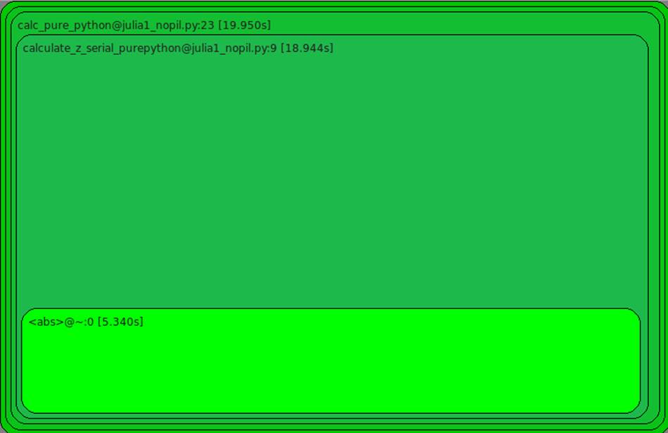
Figure 2-5. RunSnakeRun visualizing a cProfile profile file
Using line_profiler for Line-by-Line Measurements
In Ian’s opinion, Robert Kern’s line_profiler is the strongest tool for identifying the cause of CPU-bound problems in Python code. It works by profiling individual functions on a line-by-line basis, so you should start with cProfile and use the high-level view to guide which functions to profile with line_profiler.
It is worthwhile printing and annotating versions of the output from this tool as you modify your code, so you have a record of changes (successful or not) that you can quickly refer to. Don’t rely on your memory when you’re working on line-by-line changes.
To install line_profiler, issue the command pip install line_profiler.
A decorator (@profile) is used to mark the chosen function. The kernprof.py script is used to execute your code, and the CPU time and other statistics for each line of the chosen function are recorded.
NOTE
The requirement to modify the source code is a minor annoyance, as the addition of a decorator will break your unit tests unless you make a dummy decorator—see No-op @profile Decorator.
The arguments are -l for line-by-line (rather than function-level) profiling and -v for verbose output. Without -v you receive an .lprof output that you can later analyze with the line_profiler module. In Example 2-6, we’ll do a full run on our CPU-bound function.
Example 2-6. Running kernprof with line-by-line output on a decorated function to record the CPU cost of each line’s execution
$ kernprof.py -l -v julia1_lineprofiler.py
...
Wrote profile results to julia1_lineprofiler.py.lprof
Timer unit: 1e-06 s
File: julia1_lineprofiler.py
Function: calculate_z_serial_purepython at line 9
Total time: 100.81 s
Line # Hits Per Hit % Time Line Contents
==================================================
9 @profile
10 def calculate_z_serial_purepython(maxiter,
zs, cs):
11 """Calculate output list using
Julia update rule"""
12 1 6870.0 0.0 output = [0] * len(zs)
13 1000001 0.8 0.8 for i in range(len(zs)):
14 1000000 0.8 0.8 n = 0
15 1000000 0.8 0.8 z = zs[i]
16 1000000 0.8 0.8 c = cs[i]
17 34219980 1.1 36.2 while abs(z) < 2 and n < maxiter:
18 33219980 1.0 32.6 z = z * z + c
19 33219980 0.8 27.2 n += 1
20 1000000 0.9 0.9 output[i] = n
21 1 4.0 0.0 return output
Introducing kernprof.py adds a substantial amount to the runtime. In this example, calculate_z_serial_purepython takes 100 seconds; this is up from 13 seconds using simple print statements and 19 seconds using cProfile. The gain is that we get a line-by-line breakdown of where the time is spent inside the function.
The % Time column is the most helpful—we can see that 36% of the time is spent on the while testing. We don’t know whether the first statement (abs(z) < 2) is more expensive than the second (n < maxiter), though. Inside the loop, we see that the update to z is also fairly expensive. Even n += 1 is expensive! Python’s dynamic lookup machinery is at work for every loop, even though we’re using the same types for each variable in each loop—this is where compiling and type specialization (Chapter 7) give us a massive win. The creation of the output list and the updates on line 20 are relatively cheap compared to the cost of the while loop.
The obvious way to further analyze the while statement is to break it up. While there has been some discussion in the Python community around the idea of rewriting the .pyc files with more detailed information for multipart, single-line statements, we are unaware of any production tools that offer a more fine-grained analysis than line_profiler.
In Example 2-7, we break the while logic into several statements. This additional complexity will increase the runtime of the function, as we have more lines of code to execute, but it might also help us to understand the costs incurred in this part of the code.
TIP
Before you look at the code, do you think we’ll learn about the costs of the fundamental operations this way? Might other factors complicate the analysis?
Example 2-7. Breaking the compound while statement into individual statements to record the cost of each part of the original parts
$ kernprof.py -l -v julia1_lineprofiler2.py
...
Wrote profile results to julia1_lineprofiler2.py.lprof
Timer unit: 1e-06 s
File: julia1_lineprofiler2.py
Function: calculate_z_serial_purepython at line 9
Total time: 184.739 s
Line # Hits Per Hit % Time Line Contents
===================================================
9 @profile
10 def calculate_z_serial_purepython(maxiter,
zs, cs):
11 """Calculate output list using
Julia update rule"""
12 1 6831.0 0.0 output = [0] * len(zs)
13 1000001 0.8 0.4 for i in range(len(zs)):
14 1000000 0.8 0.4 n = 0
15 1000000 0.9 0.5 z = zs[i]
16 1000000 0.8 0.4 c = cs[i]
17 34219980 0.8 14.9 while True:
18 34219980 1.0 19.0 not_yet_escaped = abs(z) < 2
19 34219980 0.8 15.5 iterations_left = n < maxiter
20 34219980 0.8 15.1 if not_yet_escaped
and iterations_left:
21 33219980 1.0 17.5 z = z * z + c
22 33219980 0.9 15.3 n += 1
23 else:
24 1000000 0.8 0.4 break
25 1000000 0.9 0.5 output[i] = n
26 1 5.0 0.0 return output
This version takes 184 seconds to execute, while the previous version took 100 seconds. Other factors did complicate the analysis. In this case, having extra statements that have to be executed 34,219,980 times each slows down the code. If we hadn’t used kernprof.py to investigate the line-by-line effect of this change, we might have drawn other conclusions about the reason for the slowdown, as we’d have lacked the necessary evidence.
At this point it makes sense to step back to the earlier timeit technique to test the cost of individual expressions:
>>> z = 0+0j # a point in the middle of our image
>>> %timeit abs(z) < 2 # tested inside IPython
10000000 loops, best of 3: 119 ns per loop
>>> n = 1
>>> maxiter = 300
>>> %timeit n < maxiter
10000000 loops, best of 3: 77 ns per loop
From this simple analysis it looks as though the logic test on n is almost two times faster than the call to abs. Since the order of evaluation for Python statements is both left to right and opportunistic, it makes sense to put the cheapest test on the left side of the equation. On 1 in every 301 tests for each coordinate the n < maxiter test will be False, so Python wouldn’t need to evaluate the other side of the and operator.
We never know whether abs(z) < 2 will be False until we evaluate it, and our earlier observations for this region of the complex plane suggest it is True around 10% of the time for all 300 iterations. If we wanted to have a strong understanding of the time complexity of this part of the code, it would make sense to continue the numerical analysis. In this situation, however, we want an easy check to see if we can get a quick win.
We can form a new hypothesis stating, “By swapping the order of the operators in the while statement we will achieve a reliable speedup.” We can test this hypothesis using kernprof.py, but the additional overheads of profiling this way might add too much noise. Instead, we can use an earlier version of the code, running a test comparing while abs(z) < 2 and n < maxiter: against while n < maxiter and abs(z) < 2:.
The result was a fairly stable improvement of approximately 0.4 seconds. This result is obviously minor and is very problem-specific, though using a more suitable approach to solve this problem (e.g., swapping to using Cython or PyPy, as described in Chapter 7) would yield greater gains.
We can be confident in our result because:
§ We stated a hypothesis that was easy to test.
§ We changed our code so that only the hypothesis would be tested (never test two things at once!).
§ We gathered enough evidence to support our conclusion.
For completeness, we can run a final kernprof.py on the two main functions including our optimization to confirm that we have a full picture of the overall complexity of our code. Having swapped the two components of the while test on line 17, in Example 2-8 we see a modest improvement from 36.1% of the execution time to 35.9% (this result was stable over repeated runs).
Example 2-8. Swapping the order of the compound while statement to make the test fractionally faster
$ kernprof.py -l -v julia1_lineprofiler3.py
...
Wrote profile results to julia1_lineprofiler3.py.lprof
Timer unit: 1e-06 s
File: julia1_lineprofiler3.py
Function: calculate_z_serial_purepython at line 9
Total time: 99.7097 s
Line # Hits Per Hit % Time Line Contents
==================================================
9 @profile
10 def calculate_z_serial_purepython(maxiter,
zs, cs):
11 """Calculate output list using
Julia update rule"""
12 1 6831.0 0.0 output = [0] * len(zs)
13 1000001 0.8 0.8 for i in range(len(zs)):
14 1000000 0.8 0.8 n = 0
15 1000000 0.9 0.9 z = zs[i]
16 1000000 0.8 0.8 c = cs[i]
17 34219980 1.0 35.9 while n < maxiter and abs(z) < 2:
18 33219980 1.0 32.0 z = z * z + c
19 33219980 0.8 27.9 n += 1
20 1000000 0.9 0.9 output[i] = n
21 1 5.0 0.0 return output
As expected, we can see from the output in Example 2-9 that calculate_z_serial_purepython takes most (97%) of the time of its parent function. The list-creation steps are minor in comparison.
Example 2-9. Testing the line-by-line costs of the setup routine
File: julia1_lineprofiler3.py
Function: calc_pure_python at line 24
Total time: 195.218 s
Line # Hits Per Hit % Time Line Contents
==================================================
24 @profile
25 def calc_pure_python(draw_output,
desired_width,
max_iterations):
...
44 1 1.0 0.0 zs = []
45 1 1.0 0.0 cs = []
46 1001 1.1 0.0 for ycoord in y:
47 1001000 1.1 0.5 for xcoord in x:
48 1000000 1.5 0.8 zs.append(
complex(xcoord, ycoord))
49 1000000 1.6 0.8 cs.append(
complex(c_real, c_imag))
50
51 1 51.0 0.0 print "Length of x:", len(x)
52 1 11.0 0.0 print "Total elements:", len(zs)
53 1 6.0 0.0 start_time = time.time()
54 1 191031307.0 97.9 output =
calculate_z_serial_purepython
(max_iterations, zs, cs)
55 1 4.0 0.0 end_time = time.time()
56 1 2.0 0.0 secs = end_time - start_time
57 1 58.0 0.0 print calculate_z_serial_purepython
.func_name + " took", secs, "seconds"
58
# this sum is expected for 1000^2 grid...
59 1 9799.0 0.0 assert sum(output) == 33219980
Using memory_profiler to Diagnose Memory Usage
Just as Robert Kern’s line_profiler package measures CPU usage, the memory_profiler module by Fabian Pedregosa and Philippe Gervais measures memory usage on a line-by-line basis. Understanding the memory usage characteristics of your code allows you to ask yourself two questions:
§ Could we use less RAM by rewriting this function to work more efficiently?
§ Could we use more RAM and save CPU cycles by caching?
memory_profiler operates in a very similar way to line_profiler, but runs far more slowly. If you install the psutil package (optional but recommended), memory_profiler will run faster. Memory profiling may easily make your code run 10 to 100 times slower. In practice, you will probably use memory_profiler occasionally and line_profiler (for CPU profiling) more frequently.
Install memory_profiler with the command pip install memory_profiler (and optionally pip install psutil).
As mentioned, the implementation of memory_profiler is not as performant as the implementation of line_profiler. It may therefore make sense to run your tests on a smaller problem that completes in a useful amount of time. Overnight runs might be sensible for validation, but you need quick and reasonable iterations to diagnose problems and hypothesize solutions. The code in Example 2-10 uses the full 1,000 × 1,000 grid, and the statistics took about 1.5 hours to collect on Ian’s laptop.
NOTE
The requirement to modify the source code is a minor annoyance. As with line_profiler, a decorator (@profile) is used to mark the chosen function. This will break your unit tests unless you make a dummy decorator—see No-op @profile Decorator.
When dealing with memory allocation, you must be aware that the situation is not as clear-cut as it is with CPU usage. Generally, it is more efficient to overallocate memory to a process into a local pool that can be used at leisure, as memory allocation operations are relatively expensive. Furthermore, garbage collection is not instant, so objects may be unavailable but still in the garbage collection pool for some time.
The outcome of this is that it is hard to really understand what is happening with memory usage and release inside a Python program, as a line of code may not allocate a deterministic amount of memory as observed from outside the process. Observing the gross trend over a set of lines is likely to lead to better insight than observing the behavior of just one line.
Let’s take a look at the output from memory_profiler in Example 2-10. Inside calculate_z_serial_purepython on line 12, we see that the allocation of 1,000,000 items causes approximately 7 MB of RAM[2] to be added to this process. This does not mean that the output list is definitely 7 MB in size, just that the process grew by approximately 7 MB during the internal allocation of the list. On line 13, we see that the process grew by approximately a further 32 MB inside the loop. This can be attributed to the call to range. (RAM tracking is further discussed inExample 11-1; the difference between 7 MB and 32 MB is due to the contents of the two lists.) In the parent process on line 46, we see that the allocation of the zs and cs lists consumes approximately 79 MB. Again, it is worth noting that this is not necessarily the true size of the arrays, just the size that the process grew by once these lists had been created.
Example 2-10. memory_profiler’s result on both of our main functions, showing an unexpected memory use in calculate_z_serial_purepython
$ python -m memory_profiler julia1_memoryprofiler.py
...
Line # Mem usage Increment Line Contents
================================================
9 89.934 MiB 0.000 MiB @profile
10 def calculate_z_serial_purepython(maxiter,
zs, cs):
11 """Calculate output list using...
12 97.566 MiB 7.633 MiB output = [0] * len(zs)
13 130.215 MiB 32.648 MiB for i in range(len(zs)):
14 130.215 MiB 0.000 MiB n = 0
15 130.215 MiB 0.000 MiB z = zs[i]
16 130.215 MiB 0.000 MiB c = cs[i]
17 130.215 MiB 0.000 MiB while n < maxiter and abs(z) < 2:
18 130.215 MiB 0.000 MiB z = z * z + c
19 130.215 MiB 0.000 MiB n += 1
20 130.215 MiB 0.000 MiB output[i] = n
21 122.582 MiB -7.633 MiB return output
Line # Mem usage Increment Line Contents
================================================
24 10.574 MiB -112.008 MiB @profile
25 def calc_pure_python(draw_output,
desired_width,
max_iterations):
26 """Create a list of complex ...
27 10.574 MiB 0.000 MiB x_step = (float(x2 - x1) / ...
28 10.574 MiB 0.000 MiB y_step = (float(y1 - y2) / ...
29 10.574 MiB 0.000 MiB x = []
30 10.574 MiB 0.000 MiB y = []
31 10.574 MiB 0.000 MiB ycoord = y2
32 10.574 MiB 0.000 MiB while ycoord > y1:
33 10.574 MiB 0.000 MiB y.append(ycoord)
34 10.574 MiB 0.000 MiB ycoord += y_step
35 10.574 MiB 0.000 MiB xcoord = x1
36 10.582 MiB 0.008 MiB while xcoord < x2:
37 10.582 MiB 0.000 MiB x.append(xcoord)
38 10.582 MiB 0.000 MiB xcoord += x_step
...
44 10.582 MiB 0.000 MiB zs = []
45 10.582 MiB 0.000 MiB cs = []
46 89.926 MiB 79.344 MiB for ycoord in y:
47 89.926 MiB 0.000 MiB for xcoord in x:
48 89.926 MiB 0.000 MiB zs.append(complex(xcoord, ycoord))
49 89.926 MiB 0.000 MiB cs.append(complex(c_real, c_imag))
50
51 89.934 MiB 0.008 MiB print "Length of x:", len(x)
52 89.934 MiB 0.000 MiB print "Total elements:", len(zs)
53 89.934 MiB 0.000 MiB start_time = time.time()
54 output = calculate_z_serial...
55 122.582 MiB 32.648 MiB end_time = time.time()
...
Another way to visualize the change in memory use is to sample over time and plot the result. memory_profiler has a utility called mprof, used once to sample the memory usage and a second time to visualize the samples. It samples by time and not by line, so it barely impacts the runtime of the code.
Figure 2-6 is created using mprof run julia1_memoryprofiler.py. This writes a statistics file that is then visualized using mprof plot. Our two functions are bracketed: this shows where in time they are entered, and we can see the growth in RAM as they run. Insidecalculate_z_serial_purepython, we can see the steady increase in RAM usage throughout the execution of the function; this is caused by all the small objects (int and float types) that are created.
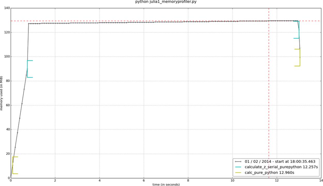
Figure 2-6. memory_profiler report using mprof
In addition to observing the behavior at the function level, we can add labels using a context manager. The snippet in Example 2-11 is used to generate the graph in Figure 2-7. We can see the create_output_list label: it appears momentarily after calculate_z_serial_purepythonand results in the process being allocated more RAM. We then pause for a second; the time.sleep(1) is an artificial addition to make the graph easier to understand.
After the label create_range_of_zs we see a large and quick increase in RAM usage; in the modified code in Example 2-11 you can see this label when we create the iterations list. Rather than using xrange, we’ve used range—the diagram should make it clear that a large list of 1,000,000 elements is instantiated just for the purposes of generating an index, and that this is an inefficient approach that will not scale to larger list sizes (we will run out of RAM!). The allocation of the memory used to hold this list will itself take a small amount of time, which contributes nothing useful to this function.
NOTE
In Python 3, the behavior of range changes—it works like xrange from Python 2. xrange is deprecated in Python 3, and the 2to3 conversion tool takes care of this change automatically.
Example 2-11. Using a context manager to add labels to the mprof graph
@profile
def calculate_z_serial_purepython(maxiter, zs, cs):
"""Calculate output list using Julia update rule"""
with profile.timestamp("create_output_list"):
output = [0] * len(zs)
time.sleep(1)
with profile.timestamp("create_range_of_zs"):
iterations = range(len(zs))
with profile.timestamp("calculate_output"):
for i initerations:
n = 0
z = zs[i]
c = cs[i]
while n < maxiter andabs(z) < 2:
z = z * z + c
n += 1
output[i] = n
return output
In the calculate_output block that runs for most of the graph, we see a very slow, linear increase in RAM usage. This will be from all of the temporary numbers used in the inner loops. Using the labels really helps us to understand at a fine-grained level where memory is being consumed.
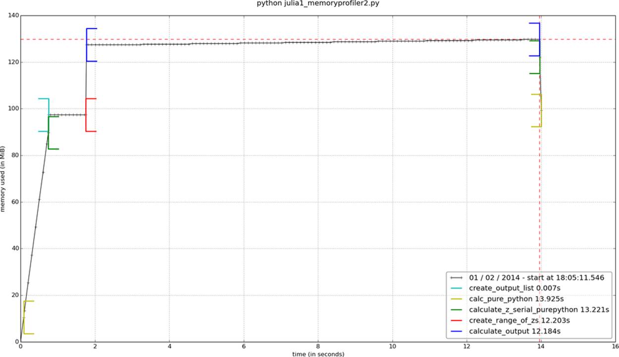
Figure 2-7. memory_profiler report using mprof with labels
Finally, we can change the range call into an xrange. In Figure 2-8, we see the corresponding decrease in RAM usage in our inner loop.
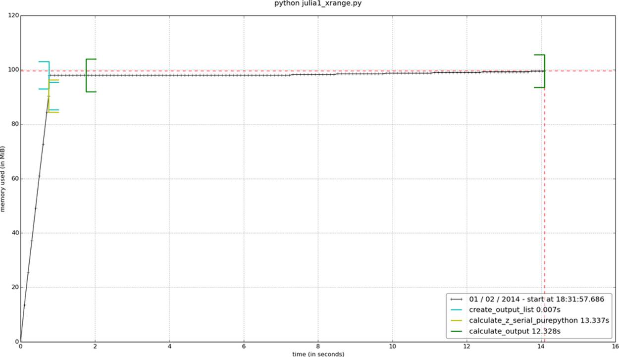
Figure 2-8. memory_profiler report showing the effect of changing range to xrange
If we want to measure the RAM used by several statements we can use the IPython magic %memit, which works just like %timeit. In Chapter 11 we will look at using %memit to measure the memory cost of lists and discuss various ways of using RAM more efficiently.
Inspecting Objects on the Heap with heapy
The Guppy project has a heap inspection tool called heapy that lets us look at the number and size of each object on Python’s heap. Looking inside the interpreter and understanding what’s held in memory is extremely useful in those rare but difficult debugging sessions where you really need to know how many objects are in use and whether they get garbage collected at appropriate times. If you have a difficult memory leak (probably because references to your objects remain hidden in a complex system), then this is the tool that’ll get you to the root of the problem.
If you’re reviewing your code to see if it is generating as many objects as you predict, you’ll find this tool very useful—the results might surprise you, and that could lead to new optimization opportunities.
To get access to heapy, install the guppy package with the command pip install guppy.
The listing in Example 2-12 is a slightly modified version of the Julia code. The heap object hpy is included in calc_pure_python, and we print out the state of the heap at three places.
Example 2-12. Using heapy to see how object counts evolve during the run of our code
def calc_pure_python(draw_output, desired_width, max_iterations):
...
while xcoord < x2:
x.append(xcoord)
xcoord += x_step
from guppy import hpy; hp = hpy()
print "heapy after creating y and x lists of floats"
h = hp.heap()
print h
zs = []
cs = []
for ycoord iny:
for xcoord inx:
zs.append(complex(xcoord, ycoord))
cs.append(complex(c_real, c_imag))
print "heapy after creating zs and cs using complex numbers"
h = hp.heap()
print h
print "Length of x:", len(x)
print "Total elements:", len(zs)
start_time = time.time()
output = calculate_z_serial_purepython(max_iterations, zs, cs)
end_time = time.time()
secs = end_time - start_time
print calculate_z_serial_purepython.func_name + " took", secs, "seconds"
print "heapy after calling calculate_z_serial_purepython"
h = hp.heap()
print h
The output in Example 2-13 shows that the memory use becomes more interesting after creating the zs and cs lists: it has grown by approximately 80 MB due to 2,000,000 complex objects consuming 64,000,000 bytes. These complex numbers represent the majority of the memory usage at this stage. If you wanted to optimize the memory usage in this program, this result would be revealing—we can see both how many objects are being stored and their overall size.
Example 2-13. Looking at the output of heapy to see how our object counts increase at each major stage of our code’s execution
$ python julia1_guppy.py
heapy after creating y and x lists of floats
Partition of a set of 27293 objects. Total size = 3416032 bytes.
Index Count % Size % Cumulative % Kind (class / dict of class)
0 10960 40 1050376 31 1050376 31 str
1 5768 21 465016 14 1515392 44 tuple
2 199 1 210856 6 1726248 51 dict of type
3 72 0 206784 6 1933032 57 dict of module
4 1592 6 203776 6 2136808 63 types.CodeType
5 313 1 201304 6 2338112 68 dict (no owner)
6 1557 6 186840 5 2524952 74 function
7 199 1 177008 5 2701960 79 type
8 124 0 135328 4 2837288 83 dict of class
9 1045 4 83600 2 2920888 86 __builtin__.wrapper_descriptor
<91 more rows. Type e.g. '_.more' to view.>
heapy after creating zs and cs using complex numbers
Partition of a set of 2027301 objects. Total size = 83671256 bytes.
Index Count % Size % Cumulative % Kind (class / dict of class)
0 2000000 99 64000000 76 64000000 76 complex
1 185 0 16295368 19 80295368 96 list
2 10962 1 1050504 1 81345872 97 str
3 5767 0 464952 1 81810824 98 tuple
4 199 0 210856 0 82021680 98 dict of type
5 72 0 206784 0 82228464 98 dict of module
6 1592 0 203776 0 82432240 99 types.CodeType
7 319 0 202984 0 82635224 99 dict (no owner)
8 1556 0 186720 0 82821944 99 function
9 199 0 177008 0 82998952 99 type
<92 more rows. Type e.g. '_.more' to view.>
Length of x: 1000
Total elements: 1000000
calculate_z_serial_purepython took 13.2436609268 seconds
heapy after calling calculate_z_serial_purepython
Partition of a set of 2127696 objects. Total size = 94207376 bytes.
Index Count % Size % Cumulative % Kind (class / dict of class)
0 2000000 94 64000000 68 64000000 68 complex
1 186 0 24421904 26 88421904 94 list
2 100965 5 2423160 3 90845064 96 int
3 10962 1 1050504 1 91895568 98 str
4 5767 0 464952 0 92360520 98 tuple
5 199 0 210856 0 92571376 98 dict of type
6 72 0 206784 0 92778160 98 dict of module
7 1592 0 203776 0 92981936 99 types.CodeType
8 319 0 202984 0 93184920 99 dict (no owner)
9 1556 0 186720 0 93371640 99 function
<92 more rows. Type e.g. '_.more' to view.>
In the third section, after calculating the Julia result, we have used 94 MB. In addition to the complex numbers we now have a large collection of integers, and more items stored in lists.
hpy.setrelheap() could be used to create a checkpoint of the memory configuration, so subsequent calls to hpy.heap() will generate a delta from this checkpoint. This way you can avoid seeing the internals of Python and prior memory setup before the point of the program that you’re analyzing.
Using dowser for Live Graphing of Instantiated Variables
Robert Brewer’s dowser hooks into the namespace of the running code and provides a real-time view of instantiated variables via a CherryPy interface in a web browser. Each object that is being tracked has an associated sparkline graphic, so you can watch to see if the quantities of certain objects are growing. This is useful for debugging long-running processes.
If you have a long-running process and you expect different memory behavior to occur depending on the actions you take in the application (e.g., with a web server you might upload data or cause complex queries to run), you can confirm this interactively. There’s an example in Figure 2-9.
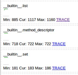
Figure 2-9. Several sparklines shown through CherryPy with dowser
To use it, we add to the Julia code a convenience function (shown in Example 2-14) that can start the CherryPy server.
Example 2-14. Helper function to start dowser in your application
def launch_memory_usage_server(port=8080):
import cherrypy
import dowser
cherrypy.tree.mount(dowser.Root())
cherrypy.config.update({
'environment': 'embedded',
'server.socket_port': port
})
cherrypy.engine.start()
Before we begin our intensive calculations we launch the CherryPy server, as shown in Example 2-15. Once we have completed our calculations we can keep the console open using the call to time.sleep—this leaves the CherryPy process running so we can continue to introspect the state of the namespace.
Example 2-15. Launching dowser at an appropriate point in our application, which will launch a web server
...
for xcoord inx:
zs.append(complex(xcoord, ycoord))
cs.append(complex(c_real, c_imag))
launch_memory_usage_server()
...
output = calculate_z_serial_purepython(max_iterations, zs, cs)
...
print "now waiting..."
while True:
time.sleep(1)
By following the TRACE links in Figure 2-9, we can view the contents of each list object (Figure 2-10). We could further drill down into each list, too—this is like using an interactive debugger in an IDE, but you can do this on a deployed server without an IDE.
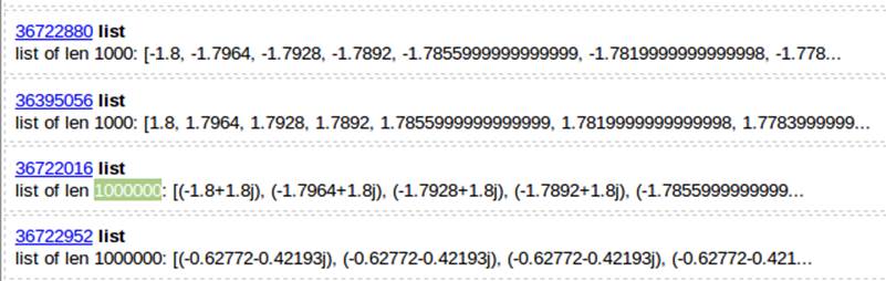
Figure 2-10. 1,000,000 items in a list with dowser
NOTE
We prefer to extract blocks of code that can be profiled in controlled conditions. Sometimes this isn’t practical, though, and sometimes you just need simpler diagnostics. Watching a live trace of a running process can be a perfect halfway house to gather the necessary evidence without doing lots of engineering.
Using the dis Module to Examine CPython Bytecode
So far we’ve reviewed various ways to measure the cost of Python code (both for CPU and RAM usage). We haven’t yet looked at the underlying bytecode used by the virtual machine, though. Understanding what’s going on “under the hood” helps to build a mental model of what’s happening in slow functions, and it’ll help when you come to compile your code. So, let’s introduce some bytecode.
The dis module lets us inspect the underlying bytecode that we run inside the stack-based CPython virtual machine. Having an understanding of what’s happening in the virtual machine that runs your higher-level Python code will help you to understand why some styles of coding are faster than others. It will also help when you come to use a tool like Cython, which steps outside of Python and generates C code.
The dis module is built in. You can pass it code or a module, and it will print out a disassembly. In Example 2-16 we disassemble the outer loop of our CPU-bound function.
TIP
You should try to disassemble one of your own functions and attempt to exactly follow how the disassembled code matches to the disassembled output. Can you match the following dis output to the original function?
Example 2-16. Using the built-in dis to understand the underlying stack-based virtual machine that runs our Python code
In [1]: import dis
In [2]: import julia1_nopil
In [3]: dis.dis(julia1_nopil.calculate_z_serial_purepython)
11 0 LOAD_CONST 1 (0)
3 BUILD_LIST 1
6 LOAD_GLOBAL 0 (len)
9 LOAD_FAST 1 (zs)
12 CALL_FUNCTION 1
15 BINARY_MULTIPLY
16 STORE_FAST 3 (output)
12 19 SETUP_LOOP 123 (to 145)
22 LOAD_GLOBAL 1 (range)
25 LOAD_GLOBAL 0 (len)
28 LOAD_FAST 1 (zs)
31 CALL_FUNCTION 1
34 CALL_FUNCTION 1
37 GET_ITER
>> 38 FOR_ITER 103 (to 144)
41 STORE_FAST 4 (i)
13 44 LOAD_CONST 1 (0)
47 STORE_FAST 5 (n)
# ...
# We'll snip the rest of the inner loop for brevity!
# ...
19 >> 131 LOAD_FAST 5 (n)
134 LOAD_FAST 3 (output)
137 LOAD_FAST 4 (i)
140 STORE_SUBSCR
141 JUMP_ABSOLUTE 38
>> 144 POP_BLOCK
20 >> 145 LOAD_FAST 3 (output)
148 RETURN_VALUE
The output is fairly straightforward, if terse. The first column contains line numbers that relate to our original file. The second column contains several >> symbols; these are the destinations for jump points elsewhere in the code. The third column is the operation address along with the operation name. The fourth column contains the parameters for the operation. The fifth column contains annotations to help line up the bytecode with the original Python parameters.
Refer back to Example 2-3 to match the bytecode to the corresponding Python code. The bytecode starts by putting the constant value 0 onto the stack, and then it builds a single-element list. Next, it searches the namespaces to find the len function, puts it on the stack, searches the namespaces again to find zs, and then puts that onto the stack. On line 12 it calls the len function from the stack, which consumes the zs reference in the stack; then it applies a binary multiply to the last two arguments (the length of zs and the single-element list) and stores the result inoutput. That’s the first line of our Python function now dealt with. Follow the next block of bytecode to understand the behavior of the second line of Python code (the outer for loop).
TIP
The jump points (>>) match to instructions like JUMP_ABSOLUTE and POP_JUMP_IF_FALSE. Go through your own disassembled function and match the jump points to the jump instructions.
Having introduced bytecode, we can now ask: what’s the bytecode and time cost of writing a function out explicitly versus using built-ins to perform the same task?
Different Approaches, Different Complexity
There should be one—and preferably only one—obvious way to do it. Although that way may not be obvious at first unless you’re Dutch…
— Tim Peters The Zen of Python
There will be various ways to express your ideas using Python. Generally it should be clear what the most sensible option is, but if your experience is primarily with an older version of Python or another programming language, then you may have other methods in mind. Some of these ways of expressing an idea may be slower than others.
You probably care more about readability than speed for most of your code, so your team can code efficiently, without being puzzled by performant but opaque code. Sometimes you will want performance, though (without sacrificing readability). Some speed testing might be what you need.
Take a look at the two code snippets in Example 2-17. They both do the same job, but the first will generate a lot of additional Python bytecode, which will cause more overhead.
Example 2-17. A naive and a more efficient way to solve the same summation problem
def fn_expressive(upper = 1000000):
total = 0
for n inxrange(upper):
total += n
return total
def fn_terse(upper = 1000000):
return sum(xrange(upper))
print "Functions return the same result:", fn_expressive() == fn_terse()
Functions return the same result:
True
Both functions calculate the sum of a range of integers. A simple rule of thumb (but one you must back up using profiling!) is that more lines of bytecode will execute more slowly than fewer equivalent lines of bytecode that use built-in functions. In Example 2-18 we use IPython’s %timeitmagic function to measure the best execution time from a set of runs.
Example 2-18. Using %timeit to test our hypothesis that using built-in functions should be faster than writing our own functions
%timeit fn_expressive()
10 loops, best of 3: 42 ms per loop
100 loops, best of 3: 12.3 ms per loop
%timeit fn_terse()
If we use the dis module to investigate the code for each function, as shown in Example 2-19, we can see that the virtual machine has 17 lines to execute with the more expressive function and only 6 to execute with the very readable but more terse second function.
Example 2-19. Using dis to view the number of bytecode instructions involved in our two functions
import dis
print fn_expressive.func_name
dis.dis(fn_expressive)
fn_expressive
2 0 LOAD_CONST 1 (0)
3 STORE_FAST 1 (total)
3 6 SETUP_LOOP 30 (to 39)
9 LOAD_GLOBAL 0 (xrange)
12 LOAD_FAST 0 (upper)
15 CALL_FUNCTION 1
18 GET_ITER
>> 19 FOR_ITER 16 (to 38)
22 STORE_FAST 2 (n)
4 25 LOAD_FAST 1 (total)
28 LOAD_FAST 2 (n)
31 INPLACE_ADD
32 STORE_FAST 1 (total)
35 JUMP_ABSOLUTE 19
>> 38 POP_BLOCK
5 >> 39 LOAD_FAST 1 (total)
42 RETURN_VALUE
print fn_terse.func_name
dis.dis(fn_terse)
fn_terse
8 0 LOAD_GLOBAL 0 (sum)
3 LOAD_GLOBAL 1 (xrange)
6 LOAD_FAST 0 (upper)
9 CALL_FUNCTION 1
12 CALL_FUNCTION 1
15 RETURN_VALUE
The difference between the two code blocks is striking. Inside fn_expressive(), we maintain two local variables and iterate over a list using a for statement. The for loop will be checking to see if a StopIteration exception has been raised on each loop. Each iteration applies thetotal.__add__ function, which will check the type of the second variable (n) on each iteration. These checks all add a little expense.
Inside fn_terse(), we call out to an optimized C list comprehension function that knows how to generate the final result without creating intermediate Python objects. This is much faster, although each iteration must still check for the types of the objects that are being added together (inChapter 4 we look at ways of fixing the type so we don’t need to check it on each iteration).
As noted previously, you must profile your code—if you just rely on this heuristic, then you will inevitably write slower code at some point. It is definitely worth learning if Python has a shorter and still readable way to solve your problem built in. If so, it is more likely to be easily readable by another programmer, and it will probably run faster.
Unit Testing During Optimization to Maintain Correctness
If you aren’t already unit testing your code, then you are probably hurting your longer-term productivity. Ian (blushing) is embarrassed to note that once he spent a day optimizing his code, having disabled unit tests because they were inconvenient, only to discover that his significant speedup result was due to breaking a part of the algorithm he was improving. You do not need to make this mistake even once.
In addition to unit testing, you should also strongly consider using coverage.py. It checks to see which lines of code are exercised by your tests and identifies the sections that have no coverage. This quickly lets you figure out whether you’re testing the code that you’re about to optimize, such that any mistakes that might creep in during the optimization process are quickly caught.
No-op @profile Decorator
Your unit tests will fail with a NameError exception if your code uses @profile from line_profiler or memory_profiler. The reason is that the unit test framework will not be injecting the @profile decorator into the local namespace. The no-op decorator shown here solves this problem. It is easiest to add it to the block of code that you’re testing and remove it when you’re done.
With the no-op decorator, you can run your tests without modifying the code that you’re testing. This means you can run your tests after every profile-led optimization you make so you’ll never be caught out by a bad optimization step.
Let’s say we have the trivial ex.py module shown in Example 2-20. It has a test (for nosetests) and a function that we’ve been profiling with either line_profiler or memory_profiler.
Example 2-20. Simple function and test case where we wish to use @profile
# ex.py
import unittest
@profile
def some_fn(nbr):
return nbr * 2
class TestCase(unittest.TestCase):
def test(self):
result = some_fn(2)
self.assertEquals(result, 4)
If we run nosetests on our code, we’ll get a NameError:
$ nosetests ex.py
E
======================================================================
ERROR: Failure: NameError (name 'profile' is not defined)
...
NameError: name 'profile' is not defined
Ran 1 test in 0.001s
FAILED (errors=1)
The solution is to add a no-op decorator at the start of ex.py (you can remove it once you’re done with profiling). If the @profile decorator is not found in one of the namespaces (because line_profiler or memory_profiler is not being used), then the no-op version we’ve written is added. If line_profiler or memory_profiler has injected the new function into the namespace, then our no-op version is ignored.
For line_profiler, we can add the code in Example 2-21.
Example 2-21. line_profiler fix to add a no-op @profile decorator to the namespace while unit testing
# for line_profiler
if '__builtin__' not in dir() or not hasattr(__builtin__, 'profile'):
def profile(func):
def inner(*args, **kwargs):
return func(*args, **kwargs)
return inner
The __builtin__ test is for nosetests, and the hasattr test is for identifying when the @profile decorator has been injected into the namespace. We can now run nosetests on our code successfully:
$ kernprof.py -v -l ex.py
Line # Hits Time Per %%HTMLit % Time Line Contents
==============================================================
11 @profile
12 def some_fn(nbr):
13 1 3 3.0 100.0 return nbr * 2
$ nosetests ex.py
.
Ran 1 test in 0.000s
For memory_profiler, we use the code in Example 2-22.
Example 2-22. memory_profiler fix to add a no-op @profile decorator to the namespace while unit testing
# for memory_profiler
if 'profile' not in dir():
def profile(func):
def inner(*args, **kwargs):
return func(*args, **kwargs)
return inner
We’d expect it to generate output like this:
python -m memory_profiler ex.py
...
Line # Mem usage Increment Line Contents
================================================
11 10.809 MiB 0.000 MiB @profile
12 def some_fn(nbr):
13 10.809 MiB 0.000 MiB return nbr * 2
$ nosetests ex.py
.
Ran 1 test in 0.000
You can save yourself a few minutes by avoiding the use of these decorators, but once you’ve lost hours making a false optimization that breaks your code, you’ll want to integrate this into your workflow.
Strategies to Profile Your Code Successfully
Profiling requires some time and concentration. You will stand a better chance of understanding your code if you separate the section you want to test from the main body of your code. You can then unit test the code to preserve correctness, and you can pass in realistic fabricated data to exercise the inefficiencies you want to address.
Do remember to disable any BIOS-based accelerators, as they will only confuse your results. On Ian’s laptop the Intel TurboBoost feature can temporarily accelerate a CPU above its normal maximum speed if it is cool enough. This means that a cool CPU may run the same block of code faster than a hot CPU. Your operating system may also control the clock speed—a laptop on battery power is likely to more aggressively control CPU speed than a laptop on mains power. To create a more stable benchmarking configuration, we:
§ Disable TurboBoost in the BIOS.
§ Disable the operating system’s ability to override the SpeedStep (you will find this in your BIOS if you’re allowed to control it).
§ Only use mains power (never battery power).
§ Disable background tools like backups and Dropbox while running experiments.
§ Run the experiments many times to obtain a stable measurement.
§ Possibly drop to run level 1 (Unix) so that no other tasks are running.
§ Reboot and rerun the experiments to double-confirm the results.
Try to hypothesize the expected behavior of your code and then validate (or disprove!) the hypothesis with the result of a profiling step. Your choices will not change (you can only use the profiled results to drive your decisions), but your intuitive understanding of the code will improve, and this will pay off in future projects as you will be more likely to make performant decisions. Of course, you will verify these performant decisions by profiling as you go.
Do not skimp on the preparation. If you try to performance test code deep inside a larger project without separating it from the larger project, you are likely to witness side effects that will sidetrack your efforts. It is likely to be harder to unit test a larger project when you’re making fine-grained changes, and this may further hamper your efforts. Side effects could include other threads and processes impacting CPU and memory usage and network and disk activity, which will skew your results.
For web servers, investigate dowser and dozer; you can use these to visualize in real time the behavior of objects in the namespace. Definitely consider separating the code you want to test out of the main web application if possible, as this will make profiling significantly easier.
Make sure your unit tests exercise all the code paths in the code that you’re analyzing. Anything you don’t test that is used in your benchmarking may cause subtle errors that will slow down your progress. Use coverage.py to confirm that your tests are covering all the code paths.
Unit testing a complicated section of code that generates a large numerical output may be difficult. Do not be afraid to output a text file of results to run through diff or to use a pickled object. For numeric optimization problems, Ian likes to create long text files of floating-point numbers and use diff—minor rounding errors show up immediately, even if they’re rare in the output.
If your code might be subject to numerical rounding issues due to subtle changes, then you are better off with a large output that can be used for a before-and-after comparison. One cause of rounding errors is the difference in floating-point precision between CPU registers and main memory. Running your code through a different code path can cause subtle rounding errors that might later confound you—it is better to be aware of this as soon as they occur.
Obviously, it makes sense to use a source code control tool while you are profiling and optimizing. Branching is cheap, and it will preserve your sanity.
Wrap-Up
Having looked at profiling techniques, you should have all the tools you need to identify bottlenecks around CPU and RAM usage in your code. Next we’ll look at how Python implements the most common containers, so you can make sensible decisions about representing larger collections of data.
[2] memory_profiler measures memory usage according to the International Electrotechnical Commission’s MiB (mebibyte) of 2^20 bytes. This is slightly different from the more common but also more ambiguous MB (megabyte has two commonly accepted definitions!). 1 MiB is equal to 1.048576 (or approximately 1.05) MB. For the purposes of our discussion, unless dealing with very specific amounts, we’ll consider the two equivalent.