High Performance Python (2014)

Chapter 3. Lists and Tuples

QUESTIONS YOU’LL BE ABLE TO ANSWER AFTER THIS CHAPTER

§ What are lists and tuples good for?

§ What is the complexity of a lookup in a list/tuple?

§ How is that complexity achieved?

§ What are the differences between lists and tuples?

§ How does appending to a list work?

§ When should I use lists and tuples?

One of the most important things in writing efficient programs is understanding the guarantees of the data structures you use. In fact, a large part of performant programming is understanding what questions you are trying to ask of your data and picking a data structure that can answer these questions quickly. In this chapter, we will talk about the kinds of questions that lists and tuples can answer quickly, and how they do it.

Lists and tuples are a class of data structures called arrays. An array is simply a flat list of data with some intrinsic ordering. This a priori knowledge of the ordering is important: by knowing that data in our array is at a specific position, we can retrieve it in O(1)! In addition, arrays can be implemented in multiple ways. This demarcates another line between lists and tuples: lists are dynamic arrays while tuples are static arrays.

Let’s unpack these previous statements a bit. System memory on a computer can be thought of as a series of numbered buckets, each capable of holding a number. These numbers can be used to represent any variables we care about (integers, floats, strings, or other data structures), since they are simply references to where the data is located in memory.^[3^]

When we want to create an array (and thus a list or tuple), we first have to allocate a block of system memory (where every section of this block will be used as an integer-sized pointer to actual data). This involves going to kernel, the operating system’s subprocess, and requesting the use ofN consecutive buckets. Figure 3-1 shows an example of the system memory layout for an array (in this case, a list) of size six. Note that in Python lists also store how large they are, so of the six allocated blocks, only five are usable—the first element is the length.

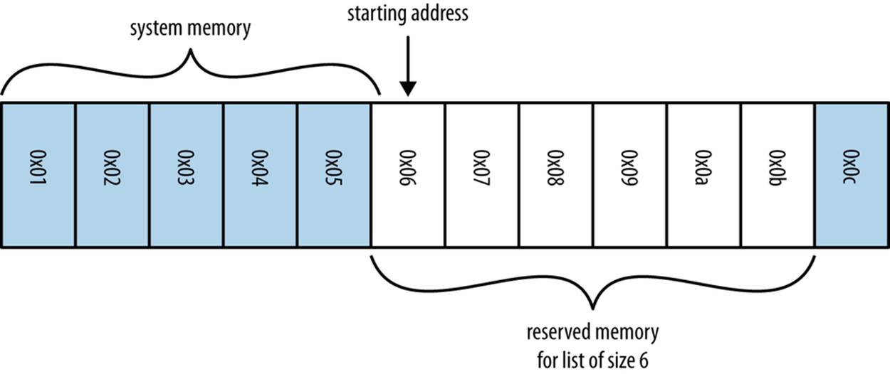
Figure 3-1. Example of system memory layout for an array of size 6

In order to look up any specific element in our list, we simply need to know which element we want and remember which bucket our data started in. Since all of the data will occupy the same amount of space (one “bucket,” or, more specifically, one integer-sized pointer to the actual data), we don’t need to know anything about the type of data that is being stored to do this calculation.

TIP

If you knew where in memory your list of N elements started, how would you find an arbitrary element in the list?

If, for example, we needed to retrieve the first element in our array, we would simply go to the first bucket in our sequence, M, and read out the value inside it. If, on the other hand, we needed the fifth element in our array, we would go to the bucket at position M+5 and read its content. In general, if we want to retrieve element i from our array, we go to bucket M+i. So, by having our data stored in consecutive buckets, and having knowledge of the ordering of our data, we can locate our data by knowing which bucket to look at in one step (or O(1)), regardless of how big our array is (Example 3-1).

Example 3-1. Timings for list lookups for lists of different sizes

>>> %%timeit l = range(10)

...: l[5]

...:

10000000 loops, best of 3: 75.5 ns per loop

>>>

>>> %%timeit l = range(10000000)

...: l[100000]

...:

10000000 loops, best of 3: 76.3 ns per loop

What if we were given an array with an unknown order and wanted to retrieve a particular element? If the ordering were known, we could simply look up that particular value. However, in this case, we must do a search operation. The most basic approach to this problem is called a “linear search,” where we iterate over every element in the array and check if it is the value we want, as seen in Example 3-2.

Example 3-2. A linear search through a list

def linear_search(needle, array):

for i, item inenumerate(array):

if item == needle:

return i

return -1

This algorithm has a worst-case performance of O(n). This case occurs when we search for something that isn’t in the array. In order to know that the element we are searching for isn’t in the array, we must first check it against every other element. Eventually, we will reach the finalreturn -1 statement. In fact, this algorithm is exactly the algorithm that list.index() uses.

The only way to increase the speed is by having some other understanding of how the data is placed in memory, or the arrangement of the buckets of data we are holding. For example, hash tables, which are a fundamental data structure powering dictionaries and sets, solve this problem inO(1) by disregarding the original ordering of the data and instead specifying another, more peculiar, organization. Alternatively, if your data is sorted in a way where every item is larger (or smaller) than its neighbor to the left (or right), then specialized search algorithms can be used that can bring your lookup time down to O(log n). This may seem like an impossible step to take from the constant-time lookups we saw before, but sometimes it is the best option (especially since search algorithms are more flexible and allow you to define searches in creative ways).

TIP

Given the following data, write an algorithm to find the index of the value 61:

[9, 18, 18, 19, 29, 42, 56, 61, 88, 95]

Since you know the data is ordered, how can you do this faster?

Hint: If you split the array in half, you know all the values on the left are smaller than the smallest element in the right set. You can use this!

A More Efficient Search

As alluded to previously, we can achieve better search performance if we first sort our data so that all elements to the left of a particular item are smaller than it (or larger). The comparison is done through the __eq__ and __lt__ magic functions of the object and can be user-defined if using custom objects.

NOTE

Without the __eq__ and __lt__ methods, a custom object will only compare to objects of the same type and the comparison will be done using the instance’s placement in memory.

The two ingredients necessary are the sorting algorithm and the searching algorithm. Python lists have a built-in sorting algorithm that uses Tim sort. Tim sort can sort through a list in O(n) in the best case (and O(n log n) in the worst case). It achieves this performance by utilizing multiple types of sorting algorithms and using heuristics to guess which algorithm will perform the best, given the data (more specifically, it hybridizes insertion and merge sort algorithms).

Once a list has been sorted, we can find our desired element using a binary search (Example 3-3), which has an average case complexity of O(log n). It achieves this by first looking at the middle of the list and comparing this value with the desired value. If this midpoint’s value is less than our desired value, then we consider the right half of the list, and we continue halving the list like this until the value is found, or until the value is known not to occur in the sorted list. As a result, we do not need to read all values in the list, as was necessary for the linear search; instead, we only read a small subset of them.

Example 3-3. Efficient searching through a sorted list—binary search

def binary_search(needle, haystack):

imin, imax = 0, len(haystack)

while True:

if imin >= imax:

return -1

midpoint = (imin + imax) // 2

if haystack[midpoint] > needle:

imax = midpoint

elif haystack[midpoint] < needle:

imin = midpoint+1

else:

return midpoint

This method allows us to find elements in a list without resorting to the potentially heavyweight solution of a dictionary. Especially when the list of data that is being operated on is intrinsically sorted, it is more efficient to simply do a binary search on the list to find an object (and get theO(log n) complexity of the search) rather than converting your data to a dictionary and then doing a lookup on it (although a dictionary lookup takes O(1), converting to a dictionary takes O(n), and a dictionary’s restriction of no repeating keys may be undesirable).

In addition, the bisect module simplifies much of this process by giving easy methods to add elements into a list while maintaining its sorting, in addition to finding elements using a heavily optimized binary search. It does this by providing alternative functions that add the element into the correct sorted placement. With the list always being sorted, we can easily find the elements we are looking for (examples of this can be found in the documentation for the bisect module). In addition, we can use bisect to find the closest element to what we are looking for very quickly (Example 3-4). This can be extremely useful for comparing two datasets that are similar but not identical.

Example 3-4. Finding close values in a list with the bisect module

import bisect

import random

def find_closest(haystack, needle):

# bisect.bisect_left will return the first value in the haystack

# that is greater than the needle

i = bisect.bisect_left(haystack, needle)

if i == len(haystack):

return i - 1

elif haystack[i] == needle:

return i

elif i > 0:

j = i - 1

# since we know the value is larger than needle (and vice versa for the

# value at j), we don't need to use absolute values here

if haystack[i] - needle > needle - haystack[j]:

return j

return i

important_numbers = []

for i inxrange(10):

new_number = random.randint(0, 1000)

bisect.insort(important_numbers, new_number)

# important_numbers will already be in order because we inserted new elements

# with bisect.insort

print important_numbers

closest_index = find_closest(important_numbers, -250)

print "Closest value to -250: ", important_numbers[closest_index]

closest_index = find_closest(important_numbers, 500)

print "Closest value to 500: ", important_numbers[closest_index]

closest_index = find_closest(important_numbers, 1100)

print "Closest value to 1100: ", important_numbers[closest_index]

In general, this touches on a fundamental rule of writing efficient code: pick the right data structure and stick with it! Although there may be more efficient data structures for particular operations, the cost of converting to those data structures may negate any efficiency boost.

Lists Versus Tuples

If lists and tuples both use the same underlying data structure, what are the differences between the two? Summarized, the main differences are:

1. Lists are dynamic arrays; they are mutable and allow for resizing (changing the number of elements that are held).

2. Tuples are static arrays; they are immutable, and the data within them cannot be changed once they have been created.

3. Tuples are cached by the Python runtime, which means that we don’t need to talk to the kernel to reserve memory every time we want to use one.

These differences outline the philosophical difference between the two: tuples are for describing multiple properties of one unchanging thing, and lists can be used to store collections of data about completely disparate objects. For example, the parts of a telephone number are perfect for a tuple: they won’t change, and if they do they represent a new object or a different phone number. Similarly, the coefficients of a polynomial fit a tuple, since different coefficients represent a different polynomial. On the other hand, the names of the people currently reading this book are better suited for a list: the data is constantly changing both in content and in size but is still always representing the same idea.

It is important to note that both lists and tuples can take mixed types. This can, as we will see, introduce quite some overhead and reduce some potential optimizations. These overheads can be removed if we force all of our data to be of the same type. In Chapter 6 we will talk about reducing both the memory used and the computational overhead by using numpy. In addition, other packages, such as blist and array, can also reduce these overheads for other, nonnumerical situations. This alludes to a major point in performant programming that we will touch on in later chapters: generic code will be much slower than code specifically designed to solve a particular problem.

In addition, the immutability of a tuple as opposed to a list, which can be resized and changed, makes it a very lightweight data structure. This means that there isn’t much overhead in memory when storing them, and operations with them are quite straightforward. With lists, as we will learn, their mutability comes at the price of extra memory needed to store them and extra computations needed when using them.

TIP

For the following example datasets, would you use a tuple or a list? Why?

1. First 20 prime numbers

2. Names of programming languages

3. A person’s age, weight, and height

4. A person’s birthday and birthplace

5. The result of a particular game of pool

6. The results of a continuing series of pool games

Solution:

1. tuple, since the data is static and will not change

2. list, since this dataset is constantly growing

3. list, since the values will need to be updated

4. tuple, since that information is static and will not change

5. tuple, since the data is static

6. list, since more games will be played (in fact, we could use a list of tuples since each individual game’s metadata will not change, but we will need to add more of them as more games are played)

Lists as Dynamic Arrays

Once we create a list, we are free to change its contents as needed:

>>> numbers = [5, 8, 1, 3, 2, 6]

>>> numbers[2] = 2*numbers[0] #

>>> numbers

[5, 8, 10, 3, 2, 6]

As described previously, this operation is O(1) because we can find the data stored within the zeroth and second elements immediately.

In addition, we can append new data to a list and grow its size:

>>> len(numbers)

6

>>> numbers.append(42)

>>> numbers

[5, 8, 10, 3, 2, 6, 42]

>>> len(numbers)

7

This is possible because dynamic arrays support a resize operation that increases the capacity of the array. When a list of size N is first appended to, Python must create a new list that is big enough to hold the original N items in addition to the extra one that is being appended. However, instead of allocating N+1 items, M items are actually allocated, where M > N, in order to provide extra headroom for future appends. Then, the data from the old list is copied to the new list and the old list is destroyed. The philosophy is that one append is probably the beginning of many appends, and by requesting extra space we can reduce the number of times this allocation must happen and thus the total number of memory copies that are necessary. This is quite important since memory copies can be quite expensive, especially when list sizes start growing. Figure 3-2shows what this overallocation looks like in Python 2.7. The formula dictating this growth is given in Example 3-5.

Example 3-5. List allocation equation in Python 2.7

M = (N >> 3) + (N < 9 ? 3 : 6)

As we append data, we utilize the extra space and increase the effective size of the list, N. As a result, N grows as we append new data until N == M. At this point, there is no extra space to insert new data into and we must create a new list with more extra space. This new list has extra headroom as given by the equation in Example 3-5, and we copy the old data into the new space.

This sequence of events is shown visually in Figure 3-3. The figure follows the various operations being performed on list l in Example 3-6.

Example 3-6. Resizing of a list

l = [1, 2]

for i inrange(3, 7):

l.append(i)

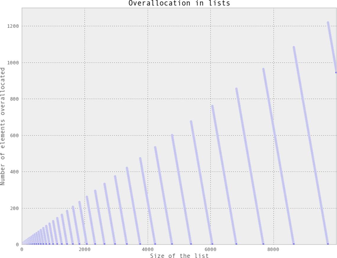
Figure 3-2. Graph showing how many extra elements are being allocated to a list of a particular size

NOTE

This extra allocation happens on the first append. When a list is directly created, as in the preceding example, only the number of elements needed is allocated.

While the amount of extra headroom allocated is generally quite small, it can add up. This effect becomes especially pronounced when you are maintaining many small lists or when keeping a particularly large list. If we are storing 1,000,000 lists, each containing 10 elements, we would suppose that 10,000,000 elements’ worth of memory is being used. In actuality, however, up to 16,000,000 elements could have been allocated if the append operator was used to construct the list. Similarly, for a large list of 100,000,000 elements, we actually have 112,500,007 elements allocated!

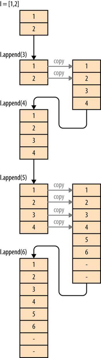
Figure 3-3. Example of how a list is mutated on multiple appends

Tuples As Static Arrays

Tuples are fixed and immutable. This means that once a tuple is created, unlike a list, it cannot be modified or resized:

>>> t = (1,2,3,4)

>>> t[0] = 5

Traceback (most recent call last):

File "<stdin>", line 1, in <module>

TypeError: 'tuple' object does not support item assignment

However, although they don’t support resizing, we can concatenate two tuples together and form a new tuple. The operation is similar to the resize operation on lists, but we do not allocate any extra space for the resulting tuple:

>>> t1 = (1,2,3,4)

>>> t2 = (5,6,7,8)

>>> t1 + t2

(1, 2, 3, 4, 5, 6, 7, 8)

If we consider this to be comparable to the append operation on lists, we see that it performs in O(n) as opposed to the O(1) speed of lists. This is because the allocate/copy operations must happen each time we add something new to the tuple, as opposed to only when our extra headroom ran out for lists. As a result of this, there is no in-place append-like operation; addition of two tuples always returns a new tuple that is in a new location in memory.

Not storing the extra headroom for resizing has the advantage of using fewer resources. A list of size 100,000,000 created with any append operation actually uses 112,500,007 elements’ worth of memory, while a tuple holding the same data will only ever use exactly 100,000,000 elements’ worth of memory. This makes tuples lightweight and preferable when data becomes static.

Furthermore, even if we create a list without append (and thus we don’t have the extra headroom introduced by an append operation), it will still be larger in memory than a tuple with the same data. This is because lists have to keep track of more information about their current state in order to efficiently resize. While this extra information is quite small (the equivalent of one extra element), it can add up if several million lists are in use.

Another benefit of the static nature of tuples is something Python does in the background: resource caching. Python is garbage collected, which means that when a variable isn’t used anymore Python frees the memory used by that variable, giving it back to the operating system for use in other applications (or for other variables). For tuples of sizes 1–20, however, when they are no longer in use the space isn’t immediately given back to the system, but rather saved for future use. This means that when a new tuple of that size is needed in the future, we don’t need to communicate with the operating system to find a region in memory to put the data, since we have a reserve of free memory already.

While this may seem like a small benefit, it is one of the fantastic things about tuples: they can be created easily and quickly since they can avoid communications with the operating system, which can cost your program quite a bit of time. Example 3-7 shows that instantiating a list can be 5.1x slower than instantiating a tuple—which can add up quite quickly if this is done in a fast loop!

Example 3-7. Instantiation timings for lists versus tuples

>>> %timeit l = [0,1,2,3,4,5,6,7,8,9]

1000000 loops, best of 3: 285 ns per loop

>>> %timeit t = (0,1,2,3,4,5,6,7,8,9)

10000000 loops, best of 3: 55.7 ns per loop

Wrap-Up

Lists and tuples are fast and low-overhead objects to use when your data already has an intrinsic ordering to it. This intrinsic ordering allows you to sidestep the search problem in these structures: if the ordering is known beforehand, then lookups are O(1), avoiding an expensive O(n) linear search. While lists can be resized, you must take care to properly understand how much overallocation is happening to ensure that the dataset can still fit in memory. On the other hand, tuples can be created quickly and without the added overhead of lists, at the cost of not being modifiable. In Aren’t Python Lists Good Enough?, we will discuss how to preallocate lists in order to alleviate some of the burden regarding frequent appends to Python lists and look at some other optimizations that can help manage these problems.

In the next chapter, we go over the computational properties of dictionaries, which solve the search/lookup problems with unordered data at the cost of overhead.