High Performance Python (2014)

Chapter 6. Matrix and Vector Computation

QUESTIONS YOU’LL BE ABLE TO ANSWER AFTER THIS CHAPTER

§ What are the bottlenecks in vector calculations?

§ What tools can I use to see how efficiently the CPU is doing my calculations?

§ Why is numpy better at numerical calculations than pure Python?

§ What are cache-misses and page-faults?

§ How can I track the memory allocations in my code?

Regardless of what problem you are trying to solve on a computer, you will encounter vector computation at some point. Vector calculations are integral to how a computer works and how it tries to speed up runtimes of programs down at the silicon level—the only thing the computer knows how to do is operate on numbers, and knowing how to do several of those calculations at once will speed up your program.

In this chapter, we try to unwrap some of the complexities of this problem by focusing on a relatively simple mathematical problem, solving the diffusion equation, and understanding what is happening at the CPU level. By understanding how different Python code affects the CPU and how to effectively probe these things, we can learn how to understand other problems as well.

We will start by introducing the problem and coming up with a quick solution using pure Python. After identifying some memory issues and trying to fix them using pure Python, we will introduce numpy and identify how and why it speeds up our code. Then we will start doing some algorithmic changes and specialize our code to solve the problem at hand. By removing some of the generality of the libraries we are using, we will yet again be able to gain more speed. Finally, we introduce some extra modules that will help facilitate this sort of process out in the field, and also explore a cautionary tale about optimizing before profiling.

Introduction to the Problem

NOTE

This section is meant to give a deeper understanding of the equations we will be solving throughout the chapter. It is not strictly necessary to understand this section in order to approach the rest of the chapter. If you wish to skip this section, make sure to look at the algorithm in Examples 6-1 and 6-2 to understand the code we will be optimizing.

On the other hand, if you read this section and want even more explanation, read Chapter 17 of Numerical Recipes, Third Edition, by William Press et al. (Cambridge University Press).

In order to explore matrix and vector computation in this chapter, we will repeatedly use the example of diffusion in fluids. Diffusion is one of the mechanisms that moves fluids and tries to make them uniformly mixed.

In this section we will explore the mathematics behind the diffusion equation. This may seem complicated, but don’t worry! We will quickly simplify this to make it more understandable. Also, it is important to note that while having a basic understanding of the final equation we are solving will be useful while reading this chapter, it is not completely necessary; the subsequent chapters will focus mainly on various formulations of the code, not the equation. However, having an understanding of the equations will help you gain intuition about ways of optimizing your code. This is true in general—understanding the motivation behind your code and the intricacies of the algorithm will give you deeper insight about possible methods of optimization.

One simple example of diffusion is dye in water: if you put several drops of dye into water at room temperature it will slowly move out until it fully mixes with the water. Since we are not stirring the water, nor is it warm enough to create convection currents, diffusion will be the main process mixing the two liquids. When solving these equations numerically, we pick what we want the initial condition to look like and are able to evolve the initial condition forward in time to see what it will look like at a later time (see Figure 6-2).

All this being said, the most important thing to know about diffusion for our purposes is its formulation. Stated as a partial differential equation in one dimension (1D), the diffusion equation is written as:

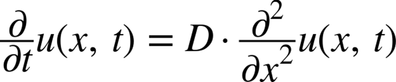
In this formulation, u is the vector representing the quantities we are diffusing. For example, we could have a vector with values of 0 where there is only water and 1 where there is only dye (and values in between where there is mixing). In general, this will be a 2D or 3D matrix representing an actual area or volume of fluid. In this way, we could have u be a 3D matrix representing the fluid in a glass, and instead of simply doing the second derivative along the x direction, we’d have to take it over all axes. In addition, D is a physical value that represents properties of the fluid we are simulating. A large value of D represents a fluid that can diffuse very easily. For simplicity, we will set D = 1 for our code, but still include it in the calculations.

NOTE

The diffusion equation is also called the heat equation. In this case, u represents the temperature of a region and D describes how well the material conducts heat. Solving the equation tells us how the heat is being transferred. So, instead of solving for how a couple of drops of dye diffuse through water, we might be solving for how the heat generated by a CPU diffuses into a heat sink.

What we will do is take the diffusion equation, which is continuous in space and time, and approximate it using discrete volumes and discrete times. We will do so using Euler’s method. Euler’s method simply takes the derivative and writes it as a difference, such that:

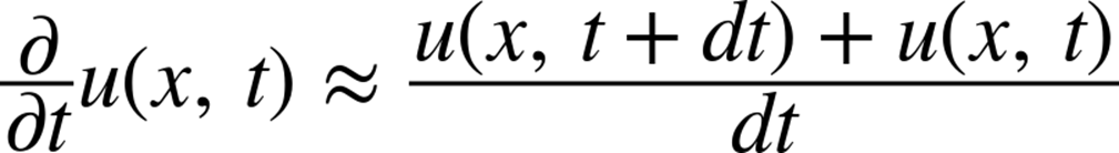
where dt is now a fixed number. This fixed number represents the time step, or the resolution in time for which we wish to solve this equation. It can be thought of as the frame rate of the movie we are trying to make. As the frame rate goes up (or dt goes down), we get a clearer picture of what happens. In fact, as dt approaches zero, Euler’s approximation becomes exact (note, however, that this exactness can only be achieved theoretically, since there is only finite precision on a computer and numerical errors will quickly dominate any results). We can thus rewrite this equation to figure out what u(x, t+dt) is given u(x,t). What this means for us is that we can start with some initial state (u(x,0), representing the glass of water just as we add a drop of dye into it) and churn through the mechanisms we’ve outlined to “evolve” that initial state and see what it will look like at future times (u(x,dt)). This type of problem is called an “initial value problem” or “Cauchy problem.”

Doing a similar trick for the derivative in x using the finite differences approximation, we arrive at the final equation:

Here, similar to how dt represents the frame rate, dx represents the resolution of the images—the smaller dx is the smaller a region every cell in our matrix represents. For simplicity, we will simply set D = 1 and dx = 1. These two values become very important when doing proper physical simulations; however, since we are simply solving the diffusion equation for illustrative purposes they are not important to us.

Using this equation, we can solve almost any diffusion problem. However, there are some considerations regarding this equation. Firstly, we said before that the spatial index in u (i.e., the x parameter) will be represented as the indices into a matrix. What happens when we try to find the value at x-dx when x is at the beginning of the matrix? This problem is called the boundary condition. You can have fixed boundary conditions that say, “any value out of the bounds of my matrix will be set to 0” (or any other value). Alternatively, you can have periodic boundary conditions that say that the values will wrap around (i.e., if one of the dimensions of your matrix has length N, the value in that dimension at index -1 is the same as at N-1, and the value at N is the same as at index 0. In other words, if you are trying to access the value at index i, you will get the value at index (i%N)).

Another consideration is how we are going to store the multiple time components of u. We could have one matrix for every time value we do our calculation for. At minimum, it seems that we will need two matrices: one for the current state of the fluid and one for the next state of the fluid. As we’ll see, there are very drastic performance considerations for this particular question.

So, what does it look like to solve this problem in practice? Example 6-1 contains some pseudocode to illustrate the way we can use our equation to solve the problem.

Example 6-1. Pseudocode for 1D diffusion

# Create the initial conditions

u = vector of length N

for i inrange(N):

u = 0 if there iswater, 1 if there isdye

# Evolve the initial conditions

D = 1

t = 0

dt = 0.0001

while True:

print "Current time is: %f" % t

unew = vector of size N

# Update step for every cell

for i inrange(N):

unew[i] = u[i] + D * dt * (u[(i+1)%N] + u[(i-1)%N] - 2 * u[i])

# Move the updated solution into u

u = unew

visualize(u)

This code will take some initial condition of the dye in water and tell us what the system looks like at every 0.0001-second interval in the future. The results of this can be seen in Figure 6-1, where we evolve our very concentrated drop of dye (represented by the top-hat function) into the future. We can see how, far into the future, the dye becomes well mixed, to the point where everywhere has a similar concentration of the dye.

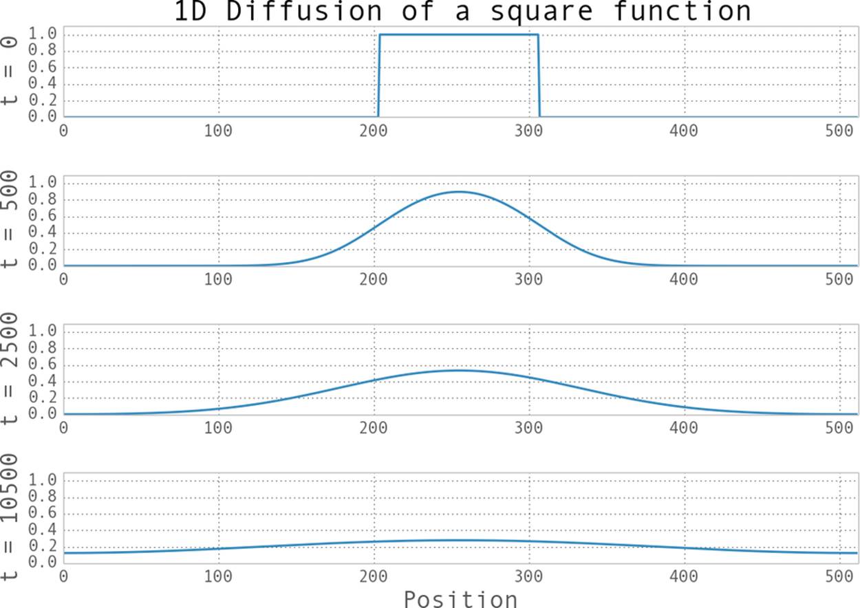
Figure 6-1. Example of 1D diffusion

For the purposes of this chapter, we will be solving the 2D version of the preceding equation. All this means is that instead of operating over a vector (or in other words, a matrix with one index), we will be operating over a 2D matrix. The only change to the equation (and thus the subsequent code) is that we must now also take the second derivative in the y direction. This simply means that the original equation we were working with becomes:

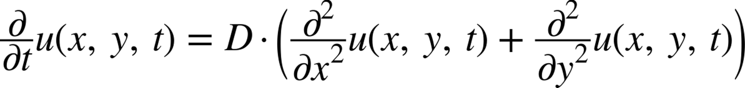
This numerical diffusion equation in 2D translates to the pseudocode in Example 6-2, using the same methods we used before.

Example 6-2. Algorithm for calculating 2D diffusion

for i inrange(N):

for j inrange(M):

unew[i][j] = u[i][j] + dt * ( \

(u[(i+1)%N][j] + u[(i-1)%N][j] - 2 * u[i][j]) + \ # d^2 u / dx^2

(u[i][(j+1)%M] + u[j][(j-1)%M] - 2 * u[i][j]) \ # d^2 u / dy^2

)

We can now put all of this together and write the full Python 2D diffusion code that we will use as the basis for our benchmarks for the rest of this chapter. While the code looks more complicated, the results are similar to that of the 1D diffusion (as can be seen in Figure 6-2).

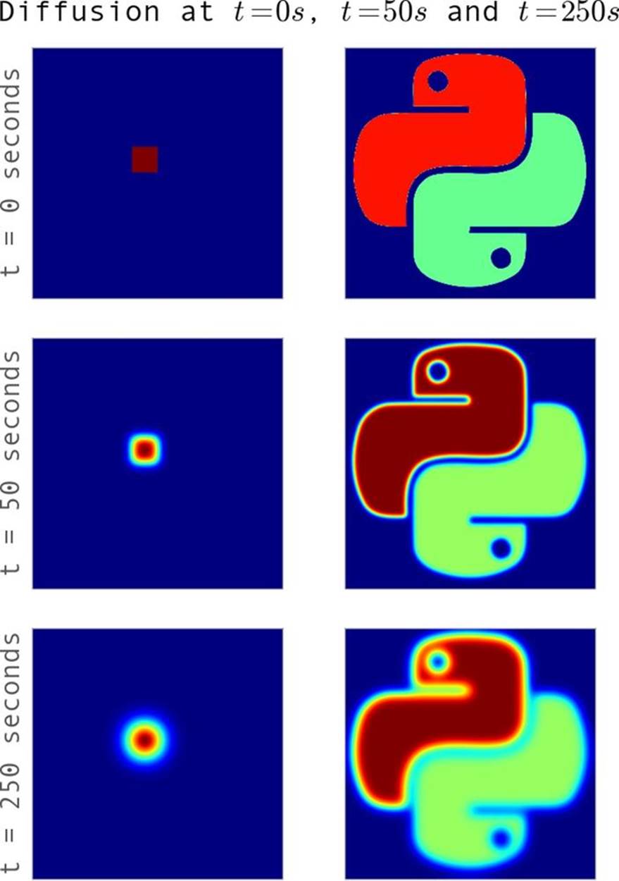
Figure 6-2. Example of diffusion for two sets of initial conditions

If you’d like to do some additional reading on the topics in this section, check out the Wikipedia page on the diffusion equation and Chapter 7 of “Numerical methods for complex systems,” by S. V. Gurevich.

Aren’t Python Lists Good Enough?

Let’s take our pseudocode from Example 6-1 and formalize it so we can better analyze its runtime performance. The first step is to write out the evolution function that takes in the matrix and returns its evolved state. This is shown in Example 6-3.

Example 6-3. Pure Python 2D diffusion

grid_shape = (1024, 1024)

def evolve(grid, dt, D=1.0):

xmax, ymax = grid_shape

new_grid = [[0.0,] * ymax for x inxrange(xmax)]

for i inxrange(xmax):

for j inxrange(ymax):

grid_xx = grid[(i+1)%xmax][j] + grid[(i-1)%xmax][j] - 2.0 * grid[i][j]

grid_yy = grid[i][(j+1)%ymax] + grid[i][(j-1)%ymax] - 2.0 * grid[i][j]

new_grid[i][j] = grid[i][j] + D * (grid_xx + grid_yy) * dt

return new_grid

NOTE

Instead of preallocating the new_grid list, we could have built it up in the for loop by using appends. While this would have been noticeably faster than what we have written, the conclusions we draw are still applicable. We chose this method because it is more illustrative.

The global variable grid_shape designates how big a region we will simulate; and, as explained in Introduction to the Problem, we are using periodic boundary conditions (which is why we use modulo for the indices). In order to actually use this code, we must initialize a grid and callevolve on it. The code in Example 6-4 is a very generic initialization procedure that will be reused throughout the chapter (its performance characteristics will not be analyzed since it must only run once, as opposed to the evolve function, which is called repeatedly).

Example 6-4. Pure Python 2D diffusion initialization

def run_experiment(num_iterations):

# Setting up initial conditions

xmax, ymax = grid_shape

grid = [[0.0,] * ymax for x inxrange(xmax)]

block_low = int(grid_shape[0] * .4)

block_high = int(grid_shape[0] * .5)

for i inxrange(block_low, block_high):

for j inxrange(block_low, block_high):

grid[i][j] = 0.005

# Evolve the initial conditions

start = time.time()

for i inrange(num_iterations):

grid = evolve(grid, 0.1)

return time.time() - start

The initial conditions used here are the same as in the square example in Figure 6-2.

The values for dt and grid elements have been chosen to be sufficiently small that the algorithm is stable. See William Press et al.’s Numerical Recipes, Third Edition, for a more in-depth treatment of this algorithm’s convergence characteristics.

Problems with Allocating Too Much

By using line_profiler on the pure Python evolution function, we can start to unravel what is contributing to a possibly slow runtime. Looking at the profiler output in Example 6-5, we see that most of the time spent in the function is spent doing the derivative calculation and updating the grid.^[9^] This is what we want, since this is a purely CPU-bound problem—any time spent not solving the CPU-bound problem is an obvious place for optimization.

Example 6-5. Pure Python 2D diffusion profiling

$ kernprof.py -lv diffusion_python.py

Wrote profile results to diffusion_python.py.lprof

Timer unit: 1e-06 s

File: diffusion_python.py

Function: evolve at line 8

Total time: 16.1398 s

Line # Hits Time Per Hit % Time Line Contents

==============================================================

8 @profile

9 def evolve(grid, dt, D=1.0):

10 10 39 3.9 0.0 xmax, ymax = grid_shape #

11 2626570 2159628 0.8 13.4 new_grid = ...

12 5130 4167 0.8 0.0 for i in xrange(xmax): #

13 2626560 2126592 0.8 13.2 for j in xrange(ymax):

14 2621440 4259164 1.6 26.4 grid_xx = ...

15 2621440 4196964 1.6 26.0 grid_yy = ...

16 2621440 3393273 1.3 21.0 new_grid[i][j] = ...

17 10 10 1.0 0.0 return grid #

This statement takes such a long time per hit because grid_shape must be retrieved from the local namespace (see Dictionaries and Namespaces for more information).

This line has 5,130 hits associated with it, which means the grid we operated over had xmax = 512. This comes from 512 evaluations for each value in xrange plus one evaluation of the termination condition of the loop, and all this happened 10 times.

This line has 10 hits associated with it, which informs us that the function was profiled over 10 runs.

However, the output also shows that we are spending 20% of our time allocating the new_grid list. This is a waste, because the properties of new_grid do not change—no matter what values we send to evolve, the new_grid list will always be the same shape and size and contain the same values. A simple optimization would be to allocate this list once and simply reuse it. This sort of optimization is similar to moving repetitive code outside of a fast loop:

from math import sin

def loop_slow(num_iterations):

"""

>>> %timeit loop_slow(int(1e4))

100 loops, best of 3: 2.67 ms per loop

"""

result = 0

for i inxrange(num_iterations):

result += i * sin(num_iterations) #

return result

def loop_fast(num_iterations):

"""

>>> %timeit loop_fast(int(1e4))

1000 loops, best of 3: 1.38 ms per loop

"""

result = 0

factor = sin(num_iterations)

for i inxrange(num_iterations):

result += i

return result * factor

The value of sin(num_iterations) doesn’t change throughout the loop, so there is no use recalculating it every time.

We can do a similar transformation to our diffusion code, as illustrated in Example 6-6. In this case, we would want to instantiate new_grid in Example 6-4 and send it in to our evolve function. That function will do the same as it did before: read the grid list and write to the new_gridlist. Then, we can simply swap new_grid with grid and continue again.

Example 6-6. Pure Python 2D diffusion after reducing memory allocations

def evolve(grid, dt, out, D=1.0):

xmax, ymax = grid_shape

for i inxrange(xmax):

for j inxrange(ymax):

grid_xx = grid[(i+1)%xmax][j] + grid[(i-1)%xmax][j] - 2.0 * grid[i][j]

grid_yy = grid[i][(j+1)%ymax] + grid[i][(j-1)%ymax] - 2.0 * grid[i][j]

out[i][j] = grid[i][j] + D * (grid_xx + grid_yy) * dt

def run_experiment(num_iterations):

# Setting up initial conditions

xmax,ymax = grid_shape

next_grid = [[0.0,] * ymax for x inxrange(xmax)]

grid = [[0.0,] * ymax for x inxrange(xmax)]

block_low = int(grid_shape[0] * .4)

block_high = int(grid_shape[0] * .5)

for i inxrange(block_low, block_high):

for j inxrange(block_low, block_high):

grid[i][j] = 0.005

start = time.time()

for i inrange(num_iterations):

evolve(grid, 0.1, next_grid)

grid, next_grid = next_grid, grid

return time.time() - start

We can see from the line profile of the modified version of the code in Example 6-7^[10^] that this small change has given us a 21% speedup. This leads us to a conclusion similar to the conclusion made during our discussion of append operations on lists (see Lists as Dynamic Arrays): memory allocations are not cheap. Every time we request memory in order to store a variable or a list, Python must take its time to talk to the operating system in order to allocate the new space, and then we must iterate over the newly allocated space to initialize it to some value. Whenever possible, reusing space that has already been allocated will give performance speedups. However, be careful when implementing these changes. While the speedups can be substantial, as always, you should profile to make sure you are achieving the results you want and are not simply polluting your code base.

Example 6-7. Line profiling Python diffusion after reducing allocations

$ kernprof.py -lv diffusion_python_memory.py

Wrote profile results to diffusion_python_memory.py.lprof

Timer unit: 1e-06 s

File: diffusion_python_memory.py

Function: evolve at line 8

Total time: 13.3209 s

Line # Hits Time Per Hit % Time Line Contents

==============================================================

8 @profile

9 def evolve(grid, dt, out, D=1.0):

10 10 15 1.5 0.0 xmax, ymax = grid_shape

11 5130 3853 0.8 0.0 for i in xrange(xmax):

12 2626560 1942976 0.7 14.6 for j in xrange(ymax):

13 2621440 4059998 1.5 30.5 grid_xx = ...

14 2621440 4038560 1.5 30.3 grid_yy = ...

15 2621440 3275454 1.2 24.6 out[i][j] = ...

Memory Fragmentation

The Python code we wrote in Example 6-6 still has a problem that is at the heart of using Python for these sorts of vectorized operations: Python doesn’t natively support vectorization. There are two reasons for this: Python lists store pointers to the actual data, and Python bytecode is not optimized for vectorization, so for loops cannot predict when using vectorization would be beneficial.

The fact that Python lists store pointers means that instead of actually holding the data we care about, lists store locations where that data can be found. For most uses, this is good because it allows us to store whatever type of data we like inside of a list. However, when it comes to vector and matrix operations, this is a source of a lot of performance degradation.

The degradation occurs because every time we want to fetch an element from the grid matrix, we must do multiple lookups. For example, doing grid[5][2] requires us to first do a list lookup for index 5 on the list grid. This will return a pointer to where the data at that location is stored. Then we need to do another list lookup on this returned object, for the element at index 2. Once we have this reference, we have the location where the actual data is stored.

The overhead for one such lookup is not big and can be, in most cases, disregarded. However, if the data we wanted was located in one contiguous block in memory, we could move all of the data in one operation instead of needing two operations for each element. This is one of the major points with data fragmentation: when your data is fragmented, you must move each piece over individually instead of moving the entire block over. This means you are invoking more memory transfer overhead, and you are forcing the CPU to wait while data is being transferred. We will see with perf just how important this is when looking at the cache-misses.

This problem of getting the right data to the CPU when it is needed is related to the so-called “Von Neumann bottleneck.” This refers to the fact that there is limited bandwidth between the memory and the CPU as a result of the tiered memory architecture that modern computers use. If we could move data infinitely fast, we would not need any cache, since the CPU could retrieve any data it needed instantly. This would be a state where the bottleneck is nonexistent.

Since we can’t move data infinitely fast, we must prefetch data from RAM and store it in smaller but faster CPU caches so that hopefully, when the CPU needs a piece of data, it will be located in a location that can be read from quickly. While this is a severely idealized way of looking at the architecture, we can still see some of the problems with it—how do we know what data will be needed in the future? The CPU does a good job with mechanisms called branch prediction and pipelining, which try to predict the next instruction and load the relevant portions of memory into the cache while still working on the current instruction. However, the best way to minimize the effects of the bottleneck is to be smart about how we allocate our memory and how we do our calculations over our data.

Probing how well memory is being moved to the CPU can be quite hard; however, in Linux the perf tool can be used to get amazing amounts of insight into how the CPU is dealing with the program being run. For example, we can run perf on the pure Python code from Example 6-6 and see just how efficiently the CPU is running our code. The results are shown in Example 6-8. Note that the output in this and the following perf examples has been truncated to fit within the margins of the page. The removed data included variances for each measurement, indicating how much the values changed throughout multiple benchmarks. This is useful for seeing how much a measured value is dependent on the actual performance characteristics of the program versus other system properties, such as other running programs using system resources.

Example 6-8. Performance counters for pure Python 2D diffusion with reduced memory allocations

$ perf stat -e cycles,stalled-cycles-frontend,stalled-cycles-backend,instructions,\

cache-references,cache-misses,branches,branch-misses,task-clock,faults,\

minor-faults,cs,migrations -r 3 python diffusion_python_memory.py

Performance counter stats for 'python diffusion_python_memory.py' (3 runs):

329,155,359,015 cycles # 3.477 GHz

76,800,457,550 stalled-cycles-frontend # 23.33% frontend cycles idle

46,556,100,820 stalled-cycles-backend # 14.14% backend cycles idle

598,135,111,009 instructions # 1.82 insns per cycle

# 0.13 stalled cycles per insn

35,497,196 cache-references # 0.375 M/sec

10,716,972 cache-misses # 30.191 % of all cache refs

133,881,241,254 branches # 1414.067 M/sec

2,891,093,384 branch-misses # 2.16% of all branches

94678.127621 task-clock # 0.999 CPUs utilized

5,439 page-faults # 0.057 K/sec

5,439 minor-faults # 0.057 K/sec

125 context-switches # 0.001 K/sec

6 CPU-migrations # 0.000 K/sec

94.749389121 seconds time elapsed

Understanding perf

Let’s take a second to understand the various performance metrics that perf is giving us and their connection to our code. The task-clock metric tells us how many clock cycles our task took. This is different from the total runtime, because if our program took 1 second to run but used two CPUs, then the task-clock would be 1000 (task-clock is generally in milliseconds). Conveniently, perf does the calculation for us and tells us, next to this metric, how many CPUs were utilized. This number isn’t exactly 1 because there were periods where the process relied on other subsystems to do instructions for it (for example, when memory was allocated).

context-switches and CPU-migrations tell us about how the program is halted in order to wait for a kernel operation to finish (such as I/O), let other applications run, or to move execution to another CPU core. When a context-switch happens, the program’s execution is halted and another program is allowed to run instead. This is a very time-intensive task and is something we would like to minimize as much as possible, but we don’t have too much control over when this happens. The kernel delegates when programs are allowed to be switched out; however, we can do things to disincentivize the kernel from moving our program. In general, the kernel suspends a program when it is doing I/O (such as reading from memory, disk, or the network). As we’ll see in later chapters, we can use asynchronous routines to make sure that our program still uses the CPU even when waiting for I/O, which will let us keep running without being context-switched. In addition, we could set the nice value of our program in order to give our program priority and stop the kernel from context switching it. Similarly, CPU-migrations happen when the program is halted and resumed on a different CPU than the one it was on before, in order to have all CPUs have the same level of utilization. This can be seen as an especially bad context switch, since not only is our program being temporarily halted, but we lose whatever data we had in the L1 cache (recall that each CPU has its own L1 cache).

A page-fault is part of the modern Unix memory allocation scheme. When memory is allocated, the kernel doesn’t do much except give the program a reference to memory. However, later, when the memory is first used, the operating system throws a minor page fault interrupt, which pauses the program that is being run and properly allocates the memory. This is called a lazy allocation system. While this method is quite an optimization over previous memory allocation systems, minor page faults are quite an expensive operation since most of the operations are done outside the scope of the program you are running. There is also a major page fault, which happens when the program requests data from a device (disk, network, etc.) that hasn’t been read yet. These are even more expensive operations, since not only do they interrupt your program, but they also involve reading from whichever device the data lives on. This sort of page fault does not generally affect CPU-bound work; however, it will be a source of pain for any program that does disk or network reads/writes.

Once we have data in memory and we reference it, the data makes its way through the various tiers of memory (see Communications Layers for a discussion of this). Whenever we reference data that is in our cache, the cache-references metric increases. If we did not already have this data in the cache and need to fetch it from RAM, this counts as a cache-miss. We won’t get a cache miss if we are reading data we have read recently (that data will still be in the cache), or data that is located near data we have recently (data is sent from RAM into the cache in chunks). Cache misses can be a source of slowdowns when it comes to CPU-bound work, since not only do we need to wait to fetch the data from RAM, but we also interrupt the flow of our execution pipeline (more on this in a second). We will be discussing how to reduce this effect by optimizing the layout of data in memory later in this chapter.

instructions tells us how many instructions our code is issuing to the CPU. Because of pipelining, these instructions can be run several at a time, which is what the insns per cycle annotation tells us. To get a better handle on this pipelining, stalled-cycles-frontend andstalled-cycles-backend tell us how many cycles our program was waiting for the frontend or backend of the pipeline to be filled. This can happen because of a cache miss, a mispredicted branch, or a resource conflict. The frontend of the pipeline is responsible for fetching the next instruction from memory and decoding it into a valid operation, while the backend is responsible for actually running the operation. With pipelining, the CPU is able to run the current operation while fetching and preparing the next one.

A branch is a time in the code where the execution flow changes. Think of an if..then statement—depending on the result of the conditional, we will either be executing one section of code or another. This is essentially a branch in the execution of the code—the next instruction in the program could be one of two things. In order to optimize this, especially with regard to the pipeline, the CPU tries to guess which direction the branch will take and preload the relevant instructions. When this prediction is incorrect, we will get some stalled-cycles and a branch-miss. Branch misses can be quite confusing and result in many strange effects (for example, some loops will run substantially faster on sorted lists than unsorted lists simply because there will be fewer branch misses).

NOTE

If you would like a more thorough explanation of what is going on at the CPU level with the various performance metrics, check out Gurpur M. Prabhu’s fantastic “Computer Architecture Tutorial.” It deals with the problems at a very low level, which gives you a good understanding of what is going on under the hood when you run your code.

Making Decisions with perf’s Output

With all this in mind, the performance metrics in Example 6-8 are telling us that while running our code, the CPU had to reference the L1/L2 cache 35,497,196 times. Of those references, 10,716,972 (or 30.191%) were requests for data that wasn’t in memory at the time and had to be retrieved. In addition, we can see that in each CPU cycle we are able to perform an average of 1.82 instructions, which tells us the total speed boost from pipelining, out-of-order execution, and hyperthreading (or any other CPU feature that lets you run more than one instruction per clock cycle).

Fragmentation increases the number of memory transfers to the CPU. Additionally, since you don’t have multiple pieces of data ready in the CPU cache when a calculation is requested, it means you cannot vectorize the calculations. As explained in Communications Layers, vectorization of computations (or having the CPU do multiple computations at a time) can only occur if we can fill the CPU cache with all the relevant data. Since the bus can only move contiguous chunks of memory, this is only possible if the grid data is stored sequentially in RAM. Since a list stores pointers to data instead of the actual data, the actual values in the grid are scattered throughout memory and cannot be copied all at once.

We can alleviate this problem by using the array module instead of lists. These objects store data sequentially in memory, so that a slice of the array actually represents a continuous range in memory. However, this doesn’t completely fix the problem—now we have data that is stored sequentially in memory, but Python still does not know how to vectorize our loops. What we would like is for any loop that does arithmetic on our array one element at a time to work on chunks of data, but as mentioned previously, there is no such bytecode optimization in Python (partly due to the extremely dynamic nature of the language).

NOTE

Why doesn’t having the data we want stored sequentially in memory automatically give us vectorization? If we looked at the raw machine code that the CPU is running, vectorized operations (such as multiplying two arrays) use a different part of the CPU, and different instructions, than non-vectorized operations. In order for Python to use these special instructions, we must have a module that was created to use them. We will soon see how numpy gives us access to these specialized instructions.

Furthermore, because of implementation details, using the array type when creating lists of data that must be iterated on is actually slower than simply creating a list. This is because the array object stores a very low-level representation of the numbers it stores, and this must be converted into a Python-compatible version before being returned to the user. This extra overhead happens every time you index an array type. That implementation decision has made the array object less suitable for math and more suitable for storing fixed-type data more efficiently in memory.

Enter numpy

In order to deal with the fragmentation we found using perf, we must find a package that can efficiently vectorize operations. Luckily, numpy has all of the features we need—it stores data in contiguous chunks of memory and supports vectorized operations on its data. As a result, any arithmetic we do on numpy arrays happens in chunks without us having to explicitly loop over each element. Not only does this make it much easier to do matrix arithmetic this way, but it is also faster. Let’s look at an example:

from array import array

import numpy

def norm_square_list(vector):

"""

>>> vector = range(1000000)

>>> %timeit norm_square_list(vector_list)

1000 loops, best of 3: 1.16 ms per loop

"""

norm = 0

for v invector:

norm += v*v

return norm

def norm_square_list_comprehension(vector):

"""

>>> vector = range(1000000)

>>> %timeit norm_square_list_comprehension(vector_list)

1000 loops, best of 3: 913 µs per loop

"""

return sum([v*v for v invector])

def norm_squared_generator_comprehension(vector):

"""

>>> vector = range(1000000)

>>> %timeit norm_square_generator_comprehension(vector_list)

1000 loops, best of 3: 747 μs per loop

"""

return sum(v*v for v invector)

def norm_square_array(vector):

"""

>>> vector = array('l', range(1000000))

>>> %timeit norm_square_array(vector_array)

1000 loops, best of 3: 1.44 ms per loop

"""

norm = 0

for v invector:

norm += v*v

return norm

def norm_square_numpy(vector):

"""

>>> vector = numpy.arange(1000000)

>>> %timeit norm_square_numpy(vector_numpy)

10000 loops, best of 3: 30.9 µs per loop

"""

return numpy.sum(vector * vector) #

def norm_square_numpy_dot(vector):

"""

>>> vector = numpy.arange(1000000)

>>> %timeit norm_square_numpy_dot(vector_numpy)

10000 loops, best of 3: 21.8 µs per loop

"""

return numpy.dot(vector, vector) #

This creates two implied loops over vector, one to do the multiplication and one to do the sum. These loops are similar to the loops from norm_square_list_comprehension, but they are executed using numpy’s optimized numerical code.

This is the preferred way of doing vector norms in numpy by using the vectorized numpy.dot operation. The less efficient norm_square_numpy code is provided for illustration.

The simpler numpy code runs 37.54x faster than norm_square_list and 29.5x faster than the “optimized” Python list comprehension. The difference in speed between the pure Python looping method and the list comprehension method shows the benefit of doing more calculation behind the scenes rather than explicitly doing it in your Python code. By performing calculations using Python’s already-built machinery, we get the speed of the native C code that Python is built on. This is also partly the same reasoning behind why we have such a drastic speedup in the numpycode: instead of using the very generalized list structure, we have a very finely tuned and specially built object for dealing with arrays of numbers.

In addition to more lightweight and specialized machinery, the numpy object also gives us memory locality and vectorized operations, which are incredibly important when dealing with numerical computations. The CPU is exceedingly fast, and most of the time simply getting it the data it needs faster is the best way to optimize code quickly. Running each function using the perf tool we looked at earlier shows that the array and pure Python functions takes ~1x10¹¹ instructions, while the numpy version takes ~3x10⁹ instructions. In addition, the array and pure Python versions have ~80% cache misses, while numpy has ~55%.

In our norm_square_numpy code, when doing vector * vector, there is an implied loop that numpy will take care of. The implied loop is the same loop we have explicitly written out in the other examples: loop over all items in vector, multiplying each item by itself. However, since we tell numpy to do this instead of explicitly writing it out in Python code, it can take advantage of all the optimizations it wants. In the background, numpy has very optimized C code that has been specifically made to take advantage of any vectorization the CPU has enabled. In addition,numpy arrays are represented sequentially in memory as low-level numerical types, which gives them the same space requirements as array objects (from the array module).

As an extra bonus, we can reformulate the problem as a dot product, which numpy supports. This gives us a single operation to calculate the value we want, as opposed to first taking the product of the two vectors and then summing them. As you can see in Figure 6-3, this operation,norm_numpy_dot, outperforms all the others by quite a substantial margin—this is thanks to the specialization of the function, and because we don’t need to store the intermediate value of vector * vector as we did in norm_numpy.

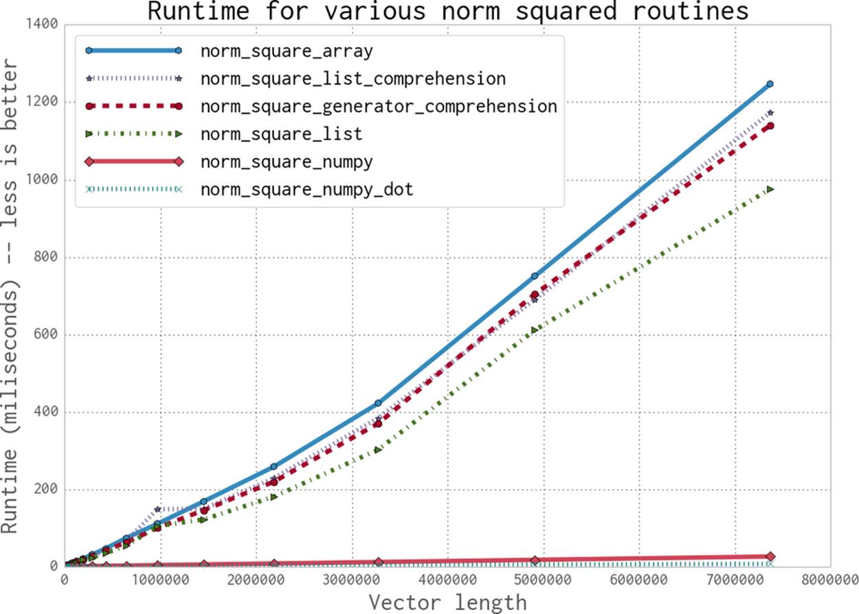
Figure 6-3. Runtimes for the various norm squared routines with vectors of different length

Applying numpy to the Diffusion Problem

Using what we’ve learned about numpy, we can easily adapt our pure Python code to be vectorized. The only new functionality we must introduce is numpy’s roll function. This function does the same thing as our modulo-index trick, but it does so for an entire numpy array. In essence, it vectorizes this reindexing:

>>> import numpy as np

>>> np.roll([1,2,3,4], 1)

array([4, 1, 2, 3])

>>> np.roll([[1,2,3],[4,5,6]], 1, axis=1)

array([[3, 1, 2],

[6, 4, 5]])

The roll function creates a new numpy array, which can be thought of as both good and bad. The downside is that we are taking time to allocate new space, which then needs to be filled with the appropriate data. On the other hand, once we have created this new rolled array we will be able to vectorize operations on it quite quickly and not suffer from cache misses from the CPU cache. This can substantially affect the speed of the actual calculation we must do on the grid. Later in this chapter, we will rewrite this so that we get the same benefit without having to constantly allocate more memory.

With this additional function we can rewrite the Python diffusion code from Example 6-6 using simpler, and vectorized, numpy arrays. In addition, we break up the calculation of the derivatives, grid_xx and grid_yy, into a separate function. Example 6-9 shows our initial numpy diffusion code.

Example 6-9. Initial numpy diffusion

import numpy as np

grid_shape = (1024, 1024)

def laplacian(grid):

return np.roll(grid, +1, 0) + np.roll(grid, -1, 0) + \

np.roll(grid, +1, 1) + np.roll(grid, -1, 1) - 4 * grid

def evolve(grid, dt, D=1):

return grid + dt * D * laplacian(grid)

def run_experiment(num_iterations):

grid = np.zeros(grid_shape)

block_low = int(grid_shape[0] * .4)

block_high = int(grid_shape[0] * .5)

grid[block_low:block_high, block_low:block_high] = 0.005

start = time.time()

for i inrange(num_iterations):

grid = evolve(grid, 0.1)

return time.time() - start

Immediately we see that this code is much shorter. This is generally a good indication of performance: we are doing a lot of the heavy lifting outside of the Python interpreter, and hopefully inside a module specially built for performance and for solving a particular problem (however, this should always be tested!). One of the assumptions here is that numpy is using better memory management in order to give the CPU the data it needs faster. However, since whether or not this happens relies on the actual implementation of numpy, let’s profile our code to see whether our hypothesis is correct. Example 6-10 shows the results.

Example 6-10. Performance counters for numpy 2D diffusion

$ perf stat -e cycles,stalled-cycles-frontend,stalled-cycles-backend,instructions,\

cache-references,cache-misses,branches,branch-misses,task-clock,faults,\

minor-faults,cs,migrations -r 3 python diffusion_numpy.py

Performance counter stats for 'python diffusion_numpy.py' (3 runs):

10,194,811,718 cycles # 3.332 GHz

4,435,850,419 stalled-cycles-frontend # 43.51% frontend cycles idle

2,055,861,567 stalled-cycles-backend # 20.17% backend cycles idle

15,165,151,844 instructions # 1.49 insns per cycle

# 0.29 stalled cycles per insn

346,798,311 cache-references # 113.362 M/sec

519,793 cache-misses # 0.150 % of all cache refs

3,506,887,927 branches # 1146.334 M/sec

3,681,441 branch-misses # 0.10% of all branches

3059.219862 task-clock # 0.999 CPUs utilized

751,707 page-faults # 0.246 M/sec

751,707 minor-faults # 0.246 M/sec

8 context-switches # 0.003 K/sec

1 CPU-migrations # 0.000 K/sec

3.061883218 seconds time elapsed

This shows that the simple change to numpy has given us a 40x speedup over the pure Python implementation with reduced memory allocations (Example 6-8). How was this achieved?

First of all, we can thank the vectorization that numpy gives. Although the numpy version seems to be running fewer instructions per cycle, each of the instructions does much more work. That is to say, one vectorized instruction can multiply four (or more) numbers in an array together instead of requiring four independent multiplication instructions. Overall this results in fewer total instructions necessary to solve the same problem.

There are also several other factors that contribute to the numpy version requiring a lower absolute number of instructions to solve the diffusion problem. One of them has to do with the full Python API being available when running the pure Python version, but not necessarily for the numpyversion—for example, the pure Python grids can be appended to in pure Python, but not in numpy. Even though we aren’t explicitly using this (or other) functionality, there is overhead in providing a system where it could be available. Since numpy can make the assumption that the data being stored is always going to be numbers, everything regarding the arrays can be optimized for operations over numbers. We will continue on the track of removing necessary functionality in favor of performance when we talk about Cython (see Cython), where it is even possible to remove list bounds checking to speed up list lookups.

Normally, the number of instructions doesn’t necessarily correlate to performance—the program with fewer instructions may not issue them efficiently, or they may be slow instructions. However, we see that in addition to reducing the number of instructions, the numpy version has also reduced a large inefficiency: cache misses (0.15% cache misses instead of 30.2%). As explained in Memory Fragmentation, cache misses slow down computations because the CPU must wait for data to be retrieved from slower memory instead of having it immediately available in its cache. In fact, memory fragmentation is such a dominant factor in performance that if we disable vectorization^[11^] in numpy but keep everything else the same, we still see a sizable speed increase compared to the pure Python version (Example 6-11).

Example 6-11. Performance counters for numpy 2D diffusion without vectorization

$ perf stat -e cycles,stalled-cycles-frontend,stalled-cycles-backend,instructions,\

cache-references,cache-misses,branches,branch-misses,task-clock,faults,\

minor-faults,cs,migrations -r 3 python diffusion_numpy.py

Performance counter stats for 'python diffusion_numpy.py' (3 runs):

48,923,515,604 cycles # 3.413 GHz

24,901,979,501 stalled-cycles-frontend # 50.90% frontend cycles idle

6,585,982,510 stalled-cycles-backend # 13.46% backend cycles idle

53,208,756,117 instructions # 1.09 insns per cycle

# 0.47 stalled cycles per insn

83,436,665 cache-references # 5.821 M/sec

1,211,229 cache-misses # 1.452 % of all cache refs

4,428,225,111 branches # 308.926 M/sec

3,716,789 branch-misses # 0.08% of all branches

14334.244888 task-clock # 0.999 CPUs utilized

751,185 page-faults # 0.052 M/sec

751,185 minor-faults # 0.052 M/sec

24 context-switches # 0.002 K/sec

5 CPU-migrations # 0.000 K/sec

14.345794896 seconds time elapsed

This shows us that the dominant factor in our 40x speedup when introducing numpy is not the vectorized instruction set, but rather the memory locality and reduced memory fragmentation. In fact, we can see from the preceding experiment that vectorization accounts for only about 15% of that 40x speedup.^[12^]

This realization that memory issues are the dominant factor in slowing down our code doesn’t come as too much of a shock. Computers are very well designed to do exactly the calculations we are requesting them to do with this problem—multiplying and adding numbers together. The bottleneck is in getting those numbers to the CPU fast enough to see it do the calculations as fast as it can.

Memory Allocations and In-Place Operations

In order to optimize the memory-dominated effects, let us try using the same method we used in Example 6-6 in order to reduce the number of allocations we make in our numpy code. Allocations are quite a bit worse than the cache misses we discussed previously. Instead of simply having to find the right data in RAM when it is not found in the cache, an allocation also must make a request to the operating system for an available chunk of data and then reserve it. The request to the operating system generates quite a lot more overhead than simply filling a cache—while filling a cache miss is a hardware routine that is optimized on the motherboard, allocating memory requires talking to another process, the kernel, in order to complete.

In order to remove the allocations in Example 6-9, we will preallocate some scratch space at the beginning of the code and then only use in-place operations. In-place operations, such as +=, *=, etc., reuse one of the inputs as their output. This means that we don’t need to allocate space to store the result of the calculation.

To show this explicitly, we will look at how the id of a numpy array changes as we perform operations on it (Example 6-12). The id is a good way of tracking this for numpy arrays, since the id has to do with what section of memory is being referenced. If two numpy arrays have the sameid, then they are referencing the same section of memory.^[13^]

Example 6-12. In-place operations reducing memory allocations

>>> import numpy as np

>>> array1 = np.random.random((10,10))

>>> array2 = np.random.random((10,10))

>>> id(array1)

140199765947424 #

>>> array1 += array2

>>> id(array1)

140199765947424 #

>>> array1 = array1 + array2

>>> id(array1)

140199765969792 #

These two ids are the same, since we are doing an in-place operation. This means that the memory address of array1 does not change; we are simply changing the data contained within it.

Here, the memory address has changed. When doing array1 + array2, a new memory address is allocated and filled with the result of the computation. This does have benefits, however, for when the original data needs to be preserved (i.e., array3 = array1 + array2 allows you to keep using array1 and array2, while in-place operations destroy some of the original data).

Furthermore, we see an expected slowdown from the non-in-place operation. For small numpy arrays, this overhead can be as much as 50% of the total computation time. For larger computations, the speedup is more in the single-percent region, but this still represents a lot of time if this is happening millions of times. In Example 6-13, we see that using in-place operations gives us a 20% speedup for small arrays. This margin will become larger as the arrays grow, since the memory allocations become more strenuous.

Example 6-13. In-place operations reducing memory allocations

>>> %%timeit array1, array2 = np.random.random((10,10)), np.random.random((10,10))

#

... array1 = array1 + array2

...

100000 loops, best of 3: 3.03 us per loop

>>> %%timeit array1, array2 = np.random.random((10,10)), np.random.random((10,10))

... array1 += array2

...

100000 loops, best of 3: 2.42 us per loop

Note that we use %%timeit instead of %timeit, which allows us to specify code to set up the experiment that doesn’t get timed.

The downside is that while rewriting our code from Example 6-9 to use in-place operations is not very complicated, it does make the resulting code a bit harder to read. In Example 6-14 we can see the results of this refactoring. We instantiate grid and next_grid vectors, and we constantly swap them with each other. grid is the current information we know about the system and, after running evolve, next_grid contains the updated information.

Example 6-14. Making most numpy operations in-place

def laplacian(grid, out):

np.copyto(out, grid)

out *= -4

out += np.roll(grid, +1, 0)

out += np.roll(grid, -1, 0)

out += np.roll(grid, +1, 1)

out += np.roll(grid, -1, 1)

def evolve(grid, dt, out, D=1):

laplacian(grid, out)

out *= D * dt

out += grid

def run_experiment(num_iterations):

next_grid = np.zeros(grid_shape)

grid = np.zeros(grid_shape)

block_low = int(grid_shape[0] * .4)

block_high = int(grid_shape[0] * .5)

grid[block_low:block_high, block_low:block_high] = 0.005

start = time.time()

for i inrange(num_iterations):

evolve(grid, 0.1, next_grid)

grid, next_grid = next_grid, grid #

return time.time() - start

Since the output of evolve gets stored in the output vector next_grid, we must swap these two variables so that, for the next iteration of the loop, grid has the most up-to-date information. This swap operation is quite cheap because only the references to the data are changed, not the data itself.

It is important to remember that since we want each operation to be in-place, whenever we do a vector operation we must have it be on its own line. This can make something as simple as A = A * B + C become quite convoluted. Since Python has a heavy emphasis on readability, we should make sure that the changes we have made give us sufficient speedups to be justified.

Comparing the performance metrics from Examples 6-15 and 6-10, we see that removing the spurious allocations sped up our code by 29%. This comes partly from a reduction in the number of cache misses, but mostly from a reduction in page faults.

Example 6-15. Performance metrics for numpy with in-place memory operations

$ perf stat -e cycles,stalled-cycles-frontend,stalled-cycles-backend,instructions,\

cache-references,cache-misses,branches,branch-misses,task-clock,faults,\

minor-faults,cs,migrations -r 3 python diffusion_numpy_memory.py

Performance counter stats for 'python diffusion_numpy_memory.py' (3 runs):

7,864,072,570 cycles # 3.330 GHz

3,055,151,931 stalled-cycles-frontend # 38.85% frontend cycles idle

1,368,235,506 stalled-cycles-backend # 17.40% backend cycles idle

13,257,488,848 instructions # 1.69 insns per cycle

# 0.23 stalled cycles per insn

239,195,407 cache-references # 101.291 M/sec

2,886,525 cache-misses # 1.207 % of all cache refs

3,166,506,861 branches # 1340.903 M/sec

3,204,960 branch-misses # 0.10% of all branches

2361.473922 task-clock # 0.999 CPUs utilized

6,527 page-faults # 0.003 M/sec

6,527 minor-faults # 0.003 M/sec

6 context-switches # 0.003 K/sec

2 CPU-migrations # 0.001 K/sec

2.363727876 seconds time elapsed

Selective Optimizations: Finding What Needs to Be Fixed

Looking at the code from Example 6-14, it seems like we have addressed most of the issues at hand: we have reduced the CPU burden by using numpy, and we have reduced the number of allocations necessary to solve the problem. However, there is always more investigation to be done. If we do a line profile on that code (Example 6-16), we see that the majority of our work is done within the laplacian function. In fact, 93% of the time evolve takes to run is spent in laplacian.

Example 6-16. Line profiling shows that laplacian is taking too much time

Wrote profile results to diffusion_numpy_memory.py.lprof

Timer unit: 1e-06 s

File: diffusion_numpy_memory.py

Function: laplacian at line 8

Total time: 3.67347 s

Line # Hits Time Per Hit % Time Line Contents

==============================================================

8 @profile

9 def laplacian(grid, out):

10 500 162009 324.0 4.4 np.copyto(out, grid)

11 500 111044 222.1 3.0 out *= -4

12 500 464810 929.6 12.7 out += np.roll(grid, +1, 0)

13 500 432518 865.0 11.8 out += np.roll(grid, -1, 0)

14 500 1261692 2523.4 34.3 out += np.roll(grid, +1, 1)

15 500 1241398 2482.8 33.8 out += np.roll(grid, -1, 1)

File: diffusion_numpy_memory.py

Function: evolve at line 17

Total time: 3.97768 s

Line # Hits Time Per Hit % Time Line Contents

==============================================================

17 @profile

18 def evolve(grid, dt, out, D=1):

19 500 3691674 7383.3 92.8 laplacian(grid, out)

20 500 111687 223.4 2.8 out *= D * dt

21 500 174320 348.6 4.4 out += grid

There could be many reasons why laplacian is so slow. However, there are two main high-level issues to consider. First, it looks like the calls to np.roll are allocating new vectors (we can verify this by looking at the documentation for the function). This means that even though we removed seven memory allocations in our previous refactoring, there are still four outstanding allocations. Furthermore, np.roll is a very generalized function that has a lot of code to deal with special cases. Since we know exactly what we want to do (move just the first column of data to be the last in every dimension), we can rewrite this function to eliminate most of the spurious code. We could even merge the np.roll logic with the add operation that happens with the rolled data to make a very specialized roll_add function that does exactly what we want with the fewest number of allocations and the least extra logic.

Example 6-17 shows what this refactoring would look like. All we need to do is create our new roll_add function and have laplacian use it. Since numpy supports fancy indexing, implementing such a function is just a matter of not jumbling up the indices. However, as stated earlier, while this code may be more performant, it is much less readable.

WARNING

Notice the extra work that has gone into having an informative docstring for the function, in addition to full tests. When you are taking a route similar to this one it is important to maintain the readability of the code, and these steps go a long way to making sure that your code is always doing what it was intended to do and that future programmers can modify your code and know what things do and when things are not working.

Example 6-17. Creating our own roll function

import numpy as np

def roll_add(rollee, shift, axis, out):

"""

Given a matrix, rollee, and an output matrix, out, this function will

perform the calculation:

>>> out += np.roll(rollee, shift, axis=axis)

This is done with the following assumptions:

* rollee is 2D

* shift will only ever be +1 or -1

* axis will only ever be 0 or 1 (also implied by the first assumption)

Using these assumptions, we are able to speed up this function by avoiding

extra machinery that numpy uses to generalize the `roll` function and also

by making this operation intrinsically in-place.

"""

if shift == 1 andaxis == 0:

out[1:, :] += rollee[:-1, :]

out[0 , :] += rollee[-1, :]

elif shift == -1 andaxis == 0:

out[:-1, :] += rollee[1:, :]

out[-1 , :] += rollee[0, :]

elif shift == 1 andaxis == 1:

out[:, 1:] += rollee[:, :-1]

out[:, 0 ] += rollee[:, -1]

elif shift == -1 andaxis == 1:

out[:, :-1] += rollee[:, 1:]

out[:, -1] += rollee[:, 0]

def test_roll_add():

rollee = np.asarray([[1,2],[3,4]])

for shift in (-1, +1):

for axis in (0, 1):

out = np.asarray([[6,3],[9,2]])

expected_result = np.roll(rollee, shift, axis=axis) + out

roll_add(rollee, shift, axis, out)

assert np.all(expected_result == out)

def laplacian(grid, out):

np.copyto(out, grid)

out *= -4

roll_add(grid, +1, 0, out)

roll_add(grid, -1, 0, out)

roll_add(grid, +1, 1, out)

roll_add(grid, -1, 1, out)

If we look at the performance counters in Example 6-18 for this rewrite, we see that while it is considerably faster than Example 6-14 (70% faster, in fact), most of the counters are about the same. The number of page-faults went down, but not by 70%. Similarly, cache-misses andcache-references went down, but not enough to account for the entire speedup. One of the most important metrics here is the instructions metric. The instructions metric counts how many CPU instructions had to be issued to run the program—in other words, how many things the CPU had to do. Somehow, the change to the customized roll_add function reduced the total number of instructions necessary by about 2.86x. This is because instead of having to rely on the entire machinery of numpy to roll our matrix, we are able to create shorter and simpler machinery that can take advantage of assumptions about our data (namely, that our data is two-dimensional and that we will only ever be rolling by 1). This theme of trimming out unnecessary machinery in both numpy and Python in general will continue in Cython.

Example 6-18. Performance metrics for numpy with in-place memory operations and custom laplacian function

$ perf stat -e cycles,stalled-cycles-frontend,stalled-cycles-backend,instructions,\

cache-references,cache-misses,branches,branch-misses,task-clock,faults,\

minor-faults,cs,migrations -r 3 python diffusion_numpy_memory2.py

Performance counter stats for 'python diffusion_numpy_memory2.py' (3 runs):

4,303,799,244 cycles # 3.108 GHz

2,814,678,053 stalled-cycles-frontend # 65.40% frontend cycles idle

1,635,172,736 stalled-cycles-backend # 37.99% backend cycles idle

4,631,882,411 instructions # 1.08 insns per cycle

# 0.61 stalled cycles per insn

272,151,957 cache-references # 196.563 M/sec

2,835,948 cache-misses # 1.042 % of all cache refs

621,565,054 branches # 448.928 M/sec

2,905,879 branch-misses # 0.47% of all branches

1384.555494 task-clock # 0.999 CPUs utilized

5,559 page-faults # 0.004 M/sec

5,559 minor-faults # 0.004 M/sec

6 context-switches # 0.004 K/sec

3 CPU-migrations # 0.002 K/sec

1.386148918 seconds time elapsed

numexpr: Making In-Place Operations Faster and Easier

One downfall of numpy’s optimization of vector operations is that it only occurs on one operation at a time. That is to say, when we are doing the operation A * B + C with numpy vectors, first the entire A * B operation completes, and the data is stored in a temporary vector; then this new vector is added with C. The in-place version of the diffusion code in Example 6-14 shows this quite explicitly.

However, there are many modules that can help with this. numexpr is a module that can take an entire vector expression and compile it into very efficient code that is optimized to minimize cache misses and temporary space used. In addition, the expressions can utilize multiple CPU cores (see Chapter 9 for more information) and specialized instructions for Intel chips to maximize the speedup.

It is very easy to change code to use numexpr: all that’s required is to rewrite the expressions as strings with references to local variables. The expressions are compiled behind the scenes (and cached so that calls to the same expression don’t incur the same cost of compilation) and run using optimized code. Example 6-19 shows the simplicity of changing the evolve function to use numexpr. In this case, we chose to use the out parameter of the evaluate function so that numexpr doesn’t allocate a new vector to which to return the result of the calculation.

Example 6-19. Using numexpr to further optimize large matrix operations

from numexpr import evaluate

def evolve(grid, dt, next_grid, D=1):

laplacian(grid, next_grid)

evaluate("next_grid*D*dt+grid", out=next_grid)

An important feature of numexpr is its consideration of CPU caches. It specifically moves data around so that the various CPU caches have the correct data in order to minimize cache misses. When we run perf on the updated code (Example 6-20), we see a speedup. However, if we look at the performance on a smaller, 512 × 512 grid (see Figure 6-4, at the end of the chapter) we see a ~15% decrease in speed. Why is this?

Example 6-20. Performance metrics for numpy with in-place memory operations, custom laplacian function, and numexpr

$ perf stat -e cycles,stalled-cycles-frontend,stalled-cycles-backend,instructions,\

cache-references,cache-misses,branches,branch-misses,task-clock,faults,\

minor-faults,cs,migrations -r 3 python diffusion_numpy_memory2_numexpr.py

Performance counter stats for 'python diffusion_numpy_memory2_numexpr.py' (3 runs):

5,940,414,581 cycles # 1.447 GHz

3,706,635,857 stalled-cycles-frontend # 62.40% frontend cycles idle

2,321,606,960 stalled-cycles-backend # 39.08% backend cycles idle

6,909,546,082 instructions # 1.16 insns per cycle

# 0.54 stalled cycles per insn

261,136,786 cache-references # 63.628 M/sec

11,623,783 cache-misses # 4.451 % of all cache refs

627,319,686 branches # 152.851 M/sec

8,443,876 branch-misses # 1.35% of all branches

4104.127507 task-clock # 1.364 CPUs utilized

9,786 page-faults # 0.002 M/sec

9,786 minor-faults # 0.002 M/sec

8,701 context-switches # 0.002 M/sec

60 CPU-migrations # 0.015 K/sec

3.009811418 seconds time elapsed

Much of the extra machinery we are bringing into our program with numexpr deals with cache considerations. When our grid size is small and all the data we need for our calculations fits in the cache, this extra machinery simply adds more instructions that don’t help performance. In addition, compiling the vector operation that we encoded as a string adds a large overhead. When the total runtime of the program is small, this overhead can be quite noticeable. However, as we increase the grid size, we should expect to see numexpr utilize our cache better than nativenumpy does. In addition, numexpr utilizes multiple cores to do its calculation and tries to saturate each of the cores’ caches. When the size of the grid is small, the extra overhead of managing the multiple cores overwhelms any possible increase in speed.

The particular computer we are running the code on has a 20,480 KB cache (Intel® Xeon® E5-2680). Since we are operating on two arrays, one for input and one for output, we can easily do the calculation for the size of the grid that will fill up our cache. The number of grid elements we can store in total is 20,480 KB / 64 bit = 2,560,000. Since we have two grids, this number is split between two objects (so each one can be at most 2,560,000 / 2 = 1,280,000 elements). Finally, taking the square root of this number gives us the size of the grid that uses that many grid elements. All in all, this means that approximately two 2D arrays of size 1,131 × 1,131 would fill up the cache (). In practice, however, we do not get to fill up the cache ourselves (other programs will fill up parts of the cache), so realistically we can probably fit two 800 × 800 arrays. Looking at Tables 6-1 and 6-2, we see that when the grid size jumps from 512 × 512 to 1,024 × 1,024, the numexpr code starts to outperform pure numpy.

A Cautionary Tale: Verify “Optimizations” (scipy)

An important thing to take away from this chapter is the approach we took to every optimization: profile the code to get a sense of what is going on, come up with a possible solution to fix slow parts, then profile to make sure the fix actually worked. Although this sounds straightforward, things can get complicated quickly, as we saw with how the performance of numexpr depended greatly on the size of the grid we were considering.

Of course, our proposed solutions don’t always work as expected. While writing the code for this chapter, this author saw that the laplacian function was the slowest routine and hypothesized that the scipy routine would be considerably faster. This thinking came from the fact that Laplacians are a common operation in image analysis and probably have a very optimized library to speed up the calls. scipy has an image submodule, so we must be in luck!

The implementation was quite simple (Example 6-21) and required little thought about the intricacies of implementing the periodic boundary conditions (or “wrap” condition, as scipy calls it).

Example 6-21. Using scipy’s laplace filter

from scipy.ndimage.filters import laplace

def laplacian(grid, out):

laplace(grid, out, mode='wrap')

Ease of implementation is quite important, and definitely won this method some points before we considered performance. However, once we benchmarked the scipy code (Example 6-22), we got the revelation: this method offers no substantial speedup compared to the code it was based on (Example 6-14). In fact, as we increase the grid size, this method starts performing worse (see Figure 6-4 at the end of the chapter).

Example 6-22. Performance metrics for diffusion with scipy’s laplace function

$ perf stat -e cycles,stalled-cycles-frontend,stalled-cycles-backend,instructions,\

cache-references,cache-misses,branches,branch-misses,task-clock,faults,\

minor-faults,cs,migrations -r 3 python diffusion_scipy.py

Performance counter stats for 'python diffusion_scipy.py' (3 runs):

6,573,168,470 cycles # 2.929 GHz

3,574,258,872 stalled-cycles-frontend # 54.38% frontend cycles idle

2,357,614,687 stalled-cycles-backend # 35.87% backend cycles idle

9,850,025,585 instructions # 1.50 insns per cycle

# 0.36 stalled cycles per insn

415,930,123 cache-references # 185.361 M/sec

3,188,390 cache-misses # 0.767 % of all cache refs

1,608,887,891 branches # 717.006 M/sec

4,017,205 branch-misses # 0.25% of all branches

2243.897843 task-clock # 0.994 CPUs utilized

7,319 page-faults # 0.003 M/sec

7,319 minor-faults # 0.003 M/sec

12 context-switches # 0.005 K/sec

1 CPU-migrations # 0.000 K/sec

2.258396667 seconds time elapsed

Comparing the performance metrics of the scipy version of the code with those of our custom laplacian function (Example 6-18), we can start to get some indication as to why we aren’t getting the speedup we were expecting from this rewrite.

The metrics that stand out the most are page-faults and instructions. Both of these values are substantially larger for the scipy version. The increase in page-faults shows us that while the scipy laplacian function has support for in-place operations, it is still allocating a lot of memory. In fact, the number of page-faults in the scipy version is larger than in our first rewrite of the numpy code (Example 6-15).

Most importantly, however, is the instructions metric. This shows us that the scipy code is requesting that the CPU do over double the amount of work as our custom laplacian code. Even though these instructions are more optimized (as we can see with the higher insns per cycle count, which says how many instructions the CPU can do in one clock cycle), the extra optimization doesn’t win out over the sheer number of added instructions. This could be in part due to the fact that the scipy code is written very generally, so that it can process all sorts of inputs with different boundary conditions (which requires extra code and thus more instructions). We can see this, in fact, by the high number of branches that the scipy code requires.

Wrap-Up

Looking back on our optimizations, we seem to have taken two main routes: reducing the time taken to get data to the CPU and reducing the amount of work that the CPU had to do. Tables 6-1 and 6-2 show a comparison of the results achieved by our various optimization efforts, for various dataset sizes, in relation to the original pure Python implementation.

Figure 6-4 shows graphically how all these methods compared to each other. We can see three bands of performance that correspond to these two methods: the band along the bottom shows the small improvement made in relation to our pure Python implementation by our first effort at reducing memory allocations, the middle band shows what happened when we used numpy and further reduced allocations, and the upper band illustrates the results achieved by reducing the work done by our process.

Table 6-1. Total runtime of all schemes for various grid sizes and 500 iterations of the evolve function

Table 6-2. Speedup compared to naive Python (Example 6-3) for all schemes and various grid sizes over 500 iterations of the evolve function

One important lesson to take away from this is that you should always take care of any administrative things the code must do during initialization. This may include allocating memory, or reading configuration from a file, or even precomputing some values that will be needed throughout the lifetime of the program. This is important for two reasons. First, you are reducing the total number of times these tasks must be done by doing them once up front, and you know that you will be able to use those resources without too much penalty in the future. Secondly, you are not disrupting the flow of the program; this allows it to pipeline more efficiently and keep the caches filled with more pertinent data.

We also learned more about the importance of data locality and how important simply getting data to the CPU is. CPU caches can be quite complicated, and often it is best to allow the various mechanisms designed to optimize them take care of the issue. However, understanding what is happening and doing all that is possible to optimize how memory is handled can make all the difference. For example, by understanding how caches work we are able to understand that the decrease in performance that leads to a saturated speedup no matter the grid size in Figure 6-4 can probably be attributed to the L3 cache being filled up by our grid. When this happens, we stop benefiting from the tiered memory approach to solving the Von Neumann bottleneck.

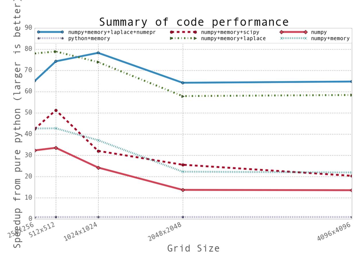
Figure 6-4. Summary of speedups from the methods attempted in this chapter

Another important lesson concerns the use of external libraries. Python is fantastic for its ease of use and readability, which allow you to write and debug code fast. However, tuning performance down to the external libraries is essential. These external libraries can be extremely fast, because they can be written in lower-level languages—but since they interface with Python, you can also still write code that used them quickly.

Finally, we learned the importance of benchmarking everything and forming hypotheses about performance before running the experiment. By forming a hypothesis before running the benchmark, we are able to form conditions to tell us whether our optimization actually worked. Was this change able to speed up runtime? Did it reduce the number of allocations? Is the number of cache misses lower? Optimization can be an art at times because of the vast complexity of computer systems, and having a quantitative probe into what is actually happening can help enormously.

One last point about optimization is that a lot of care must be taken to make sure that the optimizations you make generalize to different computers (the assumptions you make and the results of benchmarks you do may be dependent on the architecture of the computer you are running on, how the modules you are using were compiled, etc.). In addition, when making these optimizations it is incredibly important to consider other developers and how the changes will affect the readability of your code. For example, we realized that the solution we implemented in Example 6-17was potentially vague, so care was taken to make sure that the code was fully documented and tested to help not only us, but also help other people in the team.

In the next chapter we will talk about how to create your own external modules that can be finely tuned to solve specific problems with much greater efficiencies. This allows us to follow the rapid prototyping method of making our programs—first solve the problem with slow code, then identify the elements that are slow, and finally find ways to make those elements faster. By profiling often and only trying to optimize sections of code we know are slow, we can save ourselves time while still making our programs run as fast as possible.