High Performance Python (2014)
Chapter 7. Compiling to C
QUESTIONS YOU’LL BE ABLE TO ANSWER AFTER THIS CHAPTER
§ How can I have my Python code run as lower-level code?
§ What is the difference between a JIT compiler and an AOT compiler?
§ What tasks can compiled Python code perform faster than native Python?
§ Why do type annotations speed up compiled Python code?
§ How can I write modules for Python using C or Fortran?
§ How can I use libraries from C or Fortran in Python?
The easiest way to get your code to run faster is to make it do less work. Assuming you’ve already chosen good algorithms and you’ve reduced the amount of data you’re processing, the easiest way to execute fewer instructions is to compile your code down to machine code.
Python offers a number of options for this, including pure C-based compiling approaches like Cython, Shed Skin, and Pythran; LLVM-based compiling via Numba; and the replacement virtual machine PyPy, which includes a built-in just-in-time (JIT) compiler. You need to balance the requirements of code adaptability and team velocity when deciding which route to take.
Each of these tools adds a new dependency to your toolchain, and additionally Cython requires you to write in a new language type (a hybrid of Python and C), which means you need a new skill. Cython’s new language may hurt your team’s velocity, as team members without knowledge of C may have trouble supporting this code; in practice, though, this is probably a small concern as you’ll only use Cython in well-chosen, small regions of your code.
It is worth noting that performing CPU and memory profiling on your code will probably start you thinking about higher-level algorithmic optimizations that you might apply. These algorithmic changes (e.g., additional logic to avoid computations or caching to avoid recalculation) could help you avoid doing unnecessary work in your code, and Python’s expressivity helps you to spot these algorithmic opportunities. Radim Řehůřek discusses how a Python implementation can beat a pure C implementation in Making Deep Learning Fly with RadimRehurek.com.
In this chapter, we’ll review:
§ Cython—This is the most commonly used tool for compiling to C, covering both numpy and normal Python code (requires some knowledge of C)
§ Shed Skin—An automatic Python-to-C converter for non-numpy code
§ Numba—A new compiler specialized for numpy code
§ Pythran—A new compiler for both numpy and non-numpy code
§ PyPy—A stable just-in-time compiler for non-numpy code that is a replacement for the normal Python executable
Later in the chapter we’ll look at foreign function interfaces, which allow C code to be compiled into extension modules for Python. Python’s native API is used along with ctypes and cffi (from the authors of PyPy), along with the f2py Fortran-to-Python converter.
What Sort of Speed Gains Are Possible?
Gains of an order or magnitude or more are quite possible if your problem yields to a compiled approach. Here, we’ll look at various ways to achieve speedups of one to two orders of magnitude on a single core, along with using multiple cores through OpenMP.
Python code that tends to run faster after compiling is probably mathematical, and it probably has lots of loops that repeat the same operations many times. Inside these loops, you’re probably making lots of temporary objects.
Code that calls out to external libraries (e.g., regular expressions, string operations, calls to database libraries) is unlikely to show any speedup after compiling. Programs that are I/O-bound are also unlikely to show significant speedups.
Similarly, if your Python code focuses on calling vectorized numpy routines it may not run any faster after compilation—it’ll only run faster if the code being compiled is mainly Python (and probably if it is mainly looping). We looked at numpy operations in Chapter 6; compiling doesn’t really help because there aren’t many intermediate objects.
Overall, it is very unlikely that your compiled code will run any faster than a handcrafted C routine, but it is also unlikely to run much slower. It is quite possible that the generated C code from your Python will run as fast as a handwritten C routine, unless the C coder has particularly good knowledge of ways to tune the C code to the target machine’s architecture.
For math-focused code it is possible that a handcoded Fortran routine will beat an equivalent C routine, but again, this probably requires expert-level knowledge. Overall, a compiled result (probably using Cython, Pythran, or Shed Skin) will be as close to a handcoded-in-C result as most programmers will need.
Keep the diagram in Figure 7-1 in mind when you profile and work on your algorithm. A small amount of work understanding your code through profiling should enable you to make smarter choices at an algorithmic level. After this some focused work with a compiler should buy you an additional speedup. It will probably be possible to keep tweaking your algorithm, but don’t be surprised to see increasingly small improvements coming from increasingly large amounts of work on your part. Know when additional effort probably isn’t useful.
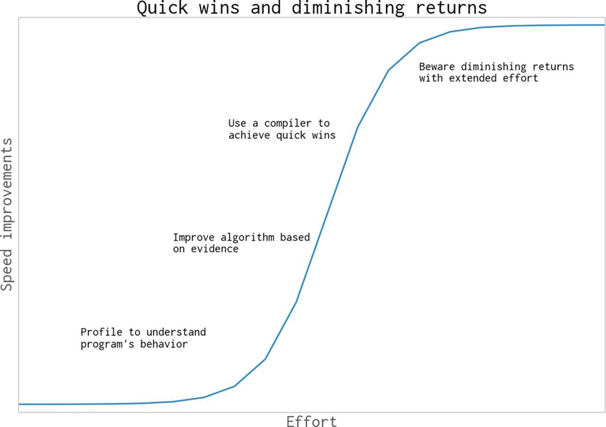
Figure 7-1. Some effort profiling and compiling brings a lot of reward, but continued effort tends to pay increasingly less
If you’re dealing with Python code and batteries-included libraries, without numpy, then Cython, Shed Skin, and PyPy are your main choices. If you’re working with numpy, then Cython, Numba, and Pythran are the right choices. These tools all support Python 2.7, and some support Python 3.2+.
Some of the following examples require a little understanding of C compilers and C code. If you lack this knowledge, then you should learn a little C and compile a working C program before diving in too deeply.
JIT Versus AOT Compilers
The tools we’ll look at roughly split into two sets: tools for compiling ahead of time (Cython, Shed Skin, Pythran) and compiling “just in time” (Numba, PyPy).
By compiling ahead of time (AOT), you create a static library that’s specialized to your machine. If you download numpy, scipy, or scikit-learn, it will compile parts of the library using Cython on your machine (or you’ll use a prebuilt compiled library if you’re using a distribution like Continuum’s Anaconda). By compiling ahead of use, you’ll have a library that can instantly be used to work on solving your problem.
By compiling just in time, you don’t have to do much (if any) work up front; you let the compiler step in to compile just the right parts of the code at the time of use. This means you have a “cold start” problem—if most of your program could be compiled and currently none of it is, when you start running your code it’ll run very slowly while it compiles. If this happens every time you run a script and you run the script many times, this cost can become significant. PyPy suffers from this problem, so you may not want to use it for short but frequently running scripts.
The current state of affairs shows us that compiling ahead of time buys us the best speedups, but often this requires the most manual effort. Just-in-time compiling offers some impressive speedups with very little manual intervention, but it can also run into the problem just described. You’ll have to consider these trade-offs when choosing the right technology for your problem.
Why Does Type Information Help the Code Run Faster?
Python is dynamically typed—a variable can refer to an object of any type, and any line of code can change the type of the object that is referred to. This makes it difficult for the virtual machine to optimize how the code is executed at the machine code level, as it doesn’t know which fundamental datatype will be used for future operations. Keeping the code generic makes it run more slowly.
In the following example, v is either a floating-point number or a pair of floating-point numbers that represent a complex number. Both conditions could occur in the same loop at different points in time, or in related serial sections of code:
v = -1.0
print type(v), abs(v)
<type 'float'> 1.0
v = 1-1j
print type(v), abs(v)
<type 'complex'> 1.41421356237
The abs function works differently depending on the underlying datatype. abs for an integer or a floating-point number simply results in turning a negative value into a positive value. abs for a complex number involves taking the square root of the sum of the squared components:
The machine code for the complex example involves more instructions and will take longer to run. Before calling abs on a variable, Python first has to look up the type of the variable and then decide which version of a function to call—this overhead adds up when you make a lot of repeated calls.
Inside Python every fundamental object, like an integer, will be wrapped up in a higher-level Python object (e.g., an int for an integer). The higher-level object has extra functions like __hash__ to assist with storage and __str__ for printing.
Inside a section of code that is CPU-bound, it is often the case that the types of variables do not change. This gives us an opportunity for static compilation and faster code execution.
If all we want are a lot of intermediate mathematical operations, then we don’t need the higher-level functions, and we may not need the machinery for reference counting either. We can drop down to the machine code level and do our calculations quickly using machine code and bytes, rather than manipulating the higher-level Python objects, which involves greater overhead. To do this we determine the types of our objects ahead of time, so we can generate the correct C code.
Using a C Compiler
In the following examples we’ll use gcc and g++ from the GNU C Compiler toolset. You could use an alternative compiler (e.g., Intel’s icc or Microsoft’s cl) if you configure your environment correctly. Cython uses gcc; Shed Skin uses g++.
gcc is a very good choice for most platforms; it is well supported and quite advanced. It is often possible to squeeze out more performance using a tuned compiler (e.g., Intel’s icc may produce faster code than gcc on Intel devices), but the cost is that you have to gain some more domain knowledge and learn how to tune the flags on the alternative compiler.
C and C++ are often used for static compilation rather than other languages like Fortran due to their ubiquity and the wide range of supporting libraries. The compiler and the converter (Cython, etc., are the converters in this case) have an opportunity to study the annotated code to determine whether static optimization steps (like inlining functions and unrolling loops) can be applied. Aggressive analysis of the intermediate abstract syntax tree (performed by Pythran, Numba, and PyPy) provides opportunities for combining knowledge of Python’s way of expressing things to inform the underlying compiler how best to take advantage of the patterns that have been seen.
Reviewing the Julia Set Example
Back in Chapter 2 we profiled the Julia set generator. This code uses integers and complex numbers to produce an output image. The calculation of the image is CPU-bound.
The main cost in the code was the CPU-bound nature of the inner loop that calculates the output list. This list can be drawn as a square pixel array, where each value represents the cost to generate that pixel.
The code for the inner function is shown in Example 7-1.
Example 7-1. Reviewing the Julia function’s CPU-bound code
def calculate_z_serial_purepython(maxiter, zs, cs):
"""Calculate output list using Julia update rule"""
output = [0] * len(zs)
for i inrange(len(zs)):
n = 0
z = zs[i]
c = cs[i]
while n < maxiter andabs(z) < 2:
z = z * z + c
n += 1
output[i] = n
return output
On Ian’s laptop the original Julia set calculation on a 1,000 × 1,000 grid with maxiter=300 takes approximately 11 seconds using a pure Python implementation running on CPython 2.7.
Cython
Cython is a compiler that converts type-annotated Python into a compiled extension module. The type annotations are C-like. This extension can be imported as a regular Python module using import. Getting started is simple, but it does have a learning curve that must be climbed with each additional level of complexity and optimization. For Ian, this is the tool of choice for turning calculation-bound functions into faster code, due to its wide usage, its maturity, and its OpenMP support.
With the OpenMP standard it is possible to convert parallel problems into multiprocessing-aware modules that run on multiple CPUs on one machine. The threads are hidden from your Python code; they operate via the generated C code.
Cython (announced in 2007) is a fork of Pyrex (announced in 2002) that expands the capabilities beyond the original aims of Pyrex. Libraries that use Cython include scipy, scikit-learn, lxml, and zmq.
Cython can be used via a setup.py script to compile a module. It can also be used interactively in IPython via a “magic” command. Typically the types are annotated by the developer, although some automated annotation is possible.
Compiling a Pure-Python Version Using Cython
The easy way to begin writing a compiled extension module involves three files. Using our Julia set as an example, they are:
§ The calling Python code (the bulk of our Julia code from earlier)
§ The function to be compiled in a new .pyx file
§ A setup.py that contains the instructions for calling Cython to make the extension module
Using this approach, the setup.py script is called to use Cython to compile the .pyx file into a compiled module. On Unix-like systems, the compiled module will probably be a .so file; on Windows it should be a .pyd (DLL-like Python library).
For the Julia example, we’ll use:
§ julia1.py to build the input lists and call the calculation function
§ cythonfn.pyx, which contains the CPU-bound function that we can annotate
§ setup.py, which contains the build instructions
The result of running setup.py is a module that can be imported. In our julia1.py script in Example 7-2 we only need to make some tiny changes to import the new module and call our function.
Example 7-2. Importing the newly compiled module into our main code
...
import calculate # as defined in setup.py
...
def calc_pure_python(desired_width, max_iterations):
# ...
start_time = time.time()
output = calculate.calculate_z(max_iterations, zs, cs)
end_time = time.time()
secs = end_time - start_time
print "Took", secs, "seconds"
...
In Example 7-3, we will start with a pure Python version without type annotations.
Example 7-3. Unmodified pure-Python code in cythonfn.pyx (renamed from .py) for Cython’s setup.py
# cythonfn.pyx
def calculate_z(maxiter, zs, cs):
"""Calculate output list using Julia update rule"""
output = [0] * len(zs)
for i inrange(len(zs)):
n = 0
z = zs[i]
c = cs[i]
while n < maxiter andabs(z) < 2:
z = z * z + c
n += 1
output[i] = n
return output
The setup.py script shown in Example 7-4 is short; it defines how to convert cythonfn.pyx into calculate.so.
Example 7-4. setup.py, which converts cythonfn.pyx into C code for compilation by Cython
from distutils.core import setup
from distutils.extension import Extension
from Cython.Distutils import build_ext
setup(
cmdclass = {'build_ext': build_ext},
ext_modules = [Extension("calculate", ["cythonfn.pyx"])]
)
When we run the setup.py script in Example 7-5 with the argument build_ext, Cython will look for cythonfn.pyx and build calculate.so.
NOTE
Remember that this is a manual step—if you update your .pyx or setup.py and forget to rerun the build command, you won’t have an updated .so module to import. If you’re unsure whether you compiled the code, check the timestamp for the .so file. If in doubt, delete the generated C files and the .so file and build them again.
Example 7-5. Running setup.py to build a new compiled module
$ python setup.py build_ext --inplace
running build_ext
cythoning cythonfn.pyx to cythonfn.c
building 'calculate' extension
gcc -pthread -fno-strict-aliasing -DNDEBUG -g -fwrapv -O2 -Wall
-Wstrict-prototypes -fPIC -I/usr/include/python2.7 -c cythonfn.c
-o build/temp.linux-x86_64-2.7/cythonfn.o
gcc -pthread -shared -Wl,-O1 -Wl,-Bsymbolic-functions -Wl,
-Bsymbolic-functions -Wl,-z,
relro build/temp.linux-x86_64-2.7/cythonfn.o -o calculate.so
The --inplace argument tells Cython to build the compiled module into the current directory rather than into a separate build directory. After the build has completed we’ll have the intermediate cythonfn.c, which is rather hard to read, along with calculate.so.
Now when the julia1.py code is run the compiled module is imported, and the Julia set is calculated on Ian’s laptop in 8.9 seconds, rather than the more usual 11 seconds. This is a small improvement for very little effort.
Cython Annotations to Analyze a Block of Code
The preceding example shows that we can quickly build a compiled module. For tight loops and mathematical operations, this alone often leads to a speedup. Obviously, we should not opimize blindly, though—we need to know what is slow so we can decide where to focus our efforts.
Cython has an annotation option that will output an HTML file that we can view in a browser. To generate the annotation we use the command cython -a cythonfn.pyx, and the output file cythonfn.html is generated. Viewed in a browser, it looks something like Figure 7-2. A similar image is available in the Cython documentation.
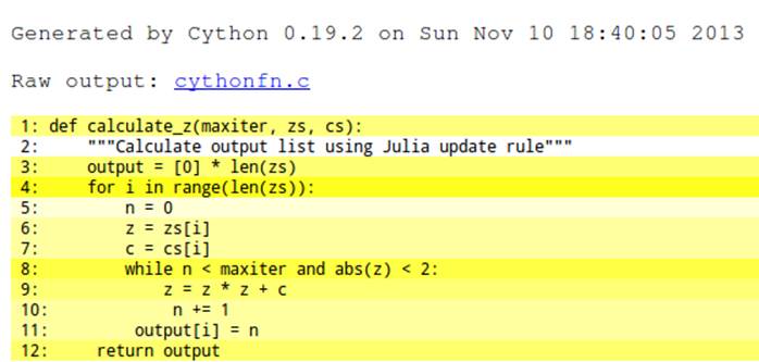
Figure 7-2. Colored Cython output of unannotated function
Each line can be expanded with a double-click to show the generated C code. More yellow means “more calls into the Python virtual machine,” while more white means “more non-Python C code.” The goal is to remove as many of the yellow lines as possible and to end up with as much white as possible.
Although “more yellow lines” means more calls into the virtual machine, this won’t necessarily cause your code to run slower. Each call into the virtual machine has a cost, but the cost of those calls will only be significant if the calls occur inside large loops. Calls outside of large loops (e.g., the line used to create output at the start of the function) are not expensive relative to the cost of the inner calculation loop. Don’t waste your time on the lines that don’t cause a slowdown.
In our example, the lines with the most calls back into the Python virtual machine (the “most yellow”) are lines 4 and 8. From our previous profiling work we know that line 8 is likely to be called over 30 million times, so that’s a great candidate to focus on.
Lines 9, 10, and 11 are almost as yellow, and we also know they’re inside the tight inner loop. In total they’ll be responsible for the bulk of the execution time of this function, so we need to focus on these first. Refer back to Using line_profiler for Line-by-Line Measurements if you need to remind yourself of how much time is spent in this section.
Lines 6 and 7 are less yellow, and since they’re only called 1 million times they’ll have a much smaller effect on the final speed, so we can focus on them later. In fact, since they are list objects there’s actually nothing we can do to speed up their access except, as you’ll see in Cython and numpy, replace the list objects with numpy arrays, which will buy a small speed advantage.
To better understand the yellow regions, you can expand each line with a double-click. In Figure 7-3 we can see that to create the output list we iterate over the length of zs, building new Python objects that are reference-counted by the Python virtual machine. Even though these calls are expensive, they won’t really affect the execution time of this function.
To improve the execution time of our function, we need to start declaring the types of objects that are involved in the expensive inner loops. These loops can then make fewer of the relatively expensive calls back into the Python virtual machine, saving us time.
In general the lines that probably cost the most CPU time are those:
§ Inside tight inner loops
§ Dereferencing list, array, or np.array items
§ Performing mathematical operations
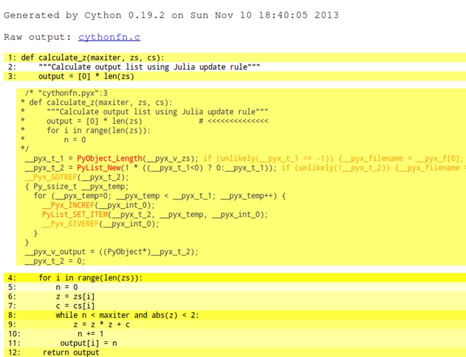
Figure 7-3. C code behind a line of Python code
NOTE
If you don’t know which lines are most frequently executed, then use a profiling tool—line_profiler, discussed in Using line_profiler for Line-by-Line Measurements, would be the most appropriate. You’ll learn which lines are executed most frequently and which lines cost the most inside the Python virtual machine, so you’ll have clear evidence of which lines you need to focus on to get the best speed gain.
Adding Some Type Annotations
Figure 7-2 showed that almost every line of our function is calling back into the Python virtual machine. All of our numeric work is also calling back into Python as we are using the higher-level Python objects. We need to convert these into local C objects, and then, after doing our numerical coding, we need to convert the result back to a Python object.
In Example 7-6 we see how to add some primitive types using the cdef syntax.
NOTE
It is important to note that these types will only be understood by Cython, and not by Python. Cython uses these types to convert the Python code to C objects, which do not have to call back into the Python stack; this means the operations run at a faster speed, but with a loss of flexibility and a loss of development speed.
The types we add are:
§ int for a signed integer
§ unsigned int for an integer that can only be positive
§ double complex for double-precision complex numbers
The cdef keyword lets us declare variables inside the function body. These must be declared at the top of the function, as that’s a requirement from the C language specification.
Example 7-6. Adding primitive C types to start making our compiled function run faster by doing more work in C and less via the Python virtual machine
def calculate_z(int maxiter, zs, cs):
"""Calculate output list using Julia update rule"""
cdef unsigned int i, n
cdef double complex z, c
output = [0] * len(zs)
for i inrange(len(zs)):
n = 0
z = zs[i]
c = cs[i]
while n < maxiter andabs(z) < 2:
z = z * z + c
n += 1
output[i] = n
return output
NOTE
When adding Cython annotations, you’re adding non-Python code to the .pyx file. This means you lose the interactive nature of developing Python in the interpreter. For those of you familiar with coding in C, we go back to the code-compile-run-debug cycle.
You might wonder if we could add a type annotation to the lists that we pass in. We can use the list keyword, but practically this has no effect for this example. The list objects still have to be interrogated at the Python level to pull out their contents, and this is very slow.
The act of giving types to some of the primitive objects is reflected in the annotated output in Figure 7-4. Critically, lines 11 and 12—two of our most frequently called lines—have now turned from yellow to white, indicating that they no longer call back to the Python virtual machine. We can anticipate a great speedup compared to the previous version. Line 10 is called over 30 million times, so we’ll still want to focus on it.
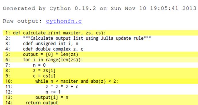
Figure 7-4. Our first type annotations
After compiling, this version takes 4.3 seconds to complete. With only a few changes to the function we are running at twice the speed of the original Python version.
It is important to note that the reason we are gaining speed is because more of the frequently performed operations are being pushed down to the C level—in this case, the updates to z and n. This means that the C compiler can optimize how the lower-level functions are operating on the bytes that represent these variables, without calling into the relatively slow Python virtual machine.
We can see in Figure 7-4 that the while loop is still somewhat expensive (it is yellow). The expensive call is in to Python for the abs function for the complex z. Cython does not provide a native abs for complex numbers; instead, we can provide our own local expansion.
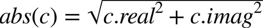
As noted earlier in this chapter, abs for a complex number involves taking the square root of the sum of the squares of the real and imaginary components. In our test, we want to see if the square root of the result is less than 2. Rather than taking the square root we can instead square the other side of the comparison, so we turn < 2 into < 4. This avoids us having to calculate the square root as the final part of the abs function.
In essence, we started with:
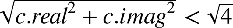
and we have simplified the operation to:

If we retained the sqrt operation in the following code, we would still see an improvement in execution speed. One of the secrets to optimizing code is to make it do as little work as possible. Removing a relatively expensive operation by considering the ultimate aim of a function means that the C compiler can focus on what it is good at, rather than trying to intuit the programmer’s ultimate needs.
Writing equivalent but more specialized code to solve the same problem is known as strength reduction. You trade worse flexibility (and possibly worse readability) for faster execution.
This mathematical unwinding leads to the next example, Example 7-7, where we have replaced the relatively expensive abs function with a simplified line of expanded mathematics.
Example 7-7. Expanding the abs function using Cython
def calculate_z(int maxiter, zs, cs):
"""Calculate output list using Julia update rule"""
cdef unsigned int i, n
cdef double complex z, c
output = [0] * len(zs)
for i inrange(len(zs)):
n = 0
z = zs[i]
c = cs[i]
while n < maxiter and (z.real * z.real + z.imag * z.imag) < 4:
z = z * z + c
n += 1
output[i] = n
return output
By annotating the code, we see a small improvement in the cost of the while statement on line 10 (Figure 7-5). Now it involves fewer calls into the Python virtual machine. It isn’t immediately obvious how much of a speed gain we’ll get, but we know that this line is called over 30 million times so we anticipate a good improvement.
This change has a dramatic effect—by reducing the number of Python calls in the innermost loop, we greatly reduce the calculation time of the function. This new version completes in just 0.25 seconds, an amazing 40x speedup over the original version.
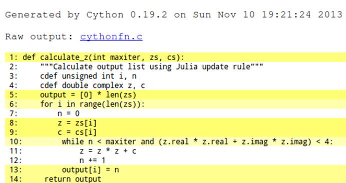
Figure 7-5. Expanded math to get a final win
NOTE
Cython supports several methods of compiling to C, some easier than the full-type-annotation method described here. You should familiarize yourself with the Pure Python Mode if you’d like an easier start to using Cython and look at pyximport to ease the introduction of Cython to colleagues.
For a final possible improvement on this piece of code, we can disable bounds checking for each dereference in the list. The goal of the bounds checking is to ensure that the program does not access data outside of the allocated array—in C it is easy to accidentally access memory outside the bounds of an array, and this will give unexpected results (and probably a segmentation fault!).
By default, Cython protects the developer from accidentally addressing outside of the list’s limits. This protection costs a little bit of CPU time, but it occurs in the outer loop of our function so in total it won’t account for much time. It is normally safe to disable bounds checking unless you are performing your own calculations for array addressing, in which case you will have to be careful to stay within the bounds of the list.
Cython has a set of flags that can be expressed in various ways. The easiest is to add them as single-line comments at the start of the .pyx file. It is also possible to use a decorator or compile-time flag to change these settings. To disable bounds checking, we add a directive for Cython inside a comment at the start of the .pyx file:
#cython: boundscheck=False
def calculate_z(int maxiter, zs, cs):
As noted, disabling the bounds checking will only save a little bit of time as it occurs in the outer loop, not in the inner loop, which is more expensive. For this example, it doesn’t save us any more time.
NOTE
Try disabling bounds checking and wraparound checking if your CPU-bound code is in a loop that is dereferencing items frequently.
Shed Skin
Shed Skin is an experimental Python-to-C++ compiler that works with Python 2.4–2.7. It uses type inference to automatically inspect a Python program to annotate the types used for each variable. This annotated code is then translated into C code for compilation with a standard compiler like g++. The automatic introspection is a very interesting feature of Shed Skin; the user only has to provide an example of how to call the function with the right kind of data, and Shed Skin will figure the rest out.
The benefit of type inference is that the programmer does not need to explicitly specify types by hand. The cost is that the analyzer has to be able to infer types for every variable in the program. In the current version, up to thousands of lines of Python can be automatically converted into C. It uses the Boehm mark-sweep garbage collector to dynamically manage memory. The Boehm garbage collector is also used in Mono and the GNU Compiler for Java. One negative for Shed Skin is that it uses external implementations for the standard libraries. Anything that has not been implemented (which includes numpy) will not be supported.
The project has over 75 examples, including many math-focused pure Python modules and even a fully working Commodore 64 emulator. Each runs significantly faster after being compiled with Shed Skin compared to running natively in CPython.
Shed Skin can build standalone executables that don’t depend on an installed Python installation or extension modules for use with import in regular Python code.
Compiled modules manage their own memory. This means that memory from a Python process is copied in and results are copied back—there is no explicit sharing of memory. For large blocks of memory (e.g., a large matrix) the cost of performing the copy may be significant; we look at this briefly toward the end of this section.
Shed Skin provides a similar set of benefits to PyPy (see PyPy). Therefore, PyPy might be easier to use, as it doesn’t require any compilation steps. The way that Shed Skin automatically adds type annotations might be interesting to some users, and the generated C may be easier to read than Cython’s generated C if you intend to modify the resulting C code. We strongly suspect that the automatic type introspection code will be of interest to other compiler writers in the community.
Building an Extension Module
For this example, we will build an extension module. We can import the generated module just as we did with the Cython examples. We could also compile this module into a standalone executable.
In Example 7-8 we have a code example in a separate module; it contains normal Python code that is not annotated in any way. Also note that we have added a __main__ test—this makes this module self-contained for type analysis. Shed Skin can use this __main__ block, which provides example arguments, to infer the types that are passed into calculate_z and from there infer the types used inside the CPU-bound function.
Example 7-8. Moving our CPU-bound function to a separate module (as we did with Cython) to allow Shed Skin’s automatic type inference system to run
# shedskinfn.py
def calculate_z(maxiter, zs, cs):
"""Calculate output list using Julia update rule"""
output = [0] * len(zs)
for i inrange(len(zs)):
n = 0
z = zs[i]
c = cs[i]
while n < maxiter andabs(z) < 2:
z = z * z + c
n += 1
output[i] = n
return output
if __name__ == "__main__":
# make a trivial example using the correct types to enable type inference
# call the function so Shed Skin can analyze the types
output = calculate_z(1, [0j], [0j])
We can import this module, as in Example 7-9, both before it has been compiled and after, in the usual way. Since the code isn’t modified (unlike with Cython), we can call the original Python module before compilation. You won’t get a speed improvement if you haven’t compiled your code, but you can debug in a lightweight way using the normal Python tools.
Example 7-9. Importing the external module to allow Shed Skin to compile just that module
...
import shedskinfn
...
def calc_pure_python(desired_width, max_iterations):
#...
start_time = time.time()
output = shedskinfn.calculate_z(max_iterations, zs, cs)
end_time = time.time()
secs = end_time - start_time
print "Took", secs, "seconds"
...
As seen in Example 7-10, we can ask Shed Skin to provide an annotated output of its analysis using shedskin -ann shedskinfn.py, and it generates shedskinfn.ss.py. We only need to “seed” the analysis with the dummy __main__ function if we’re compiling an extension module.
Example 7-10. Examining the annotated output from Shed Skin to see which types it has inferred
# shedskinfn.ss.py
def calculate_z(maxiter, zs, cs): # maxiter: [int],
# zs: [list(complex)],
# cs: [list(complex)]
"""Calculate output list using Julia update rule"""
output = [0] * len(zs) # [list(int)]
for i inrange(len(zs)): # [__iter(int)]
n = 0 # [int]
z = zs[i] # [complex]
c = cs[i] # [complex]
while n < maxiter andabs(z) < 2: # [complex]
z = z * z + c # [complex]
n += 1 # [int]
output[i] = n # [int]
return output # [list(int)]
if __name__ == "__main__": # []
# make a trivial example using the correct types to enable type inference
# call the function so Shed Skin can analyze the types
output = calculate_z(1, [0j], [0j]) # [list(int)]
The __main__ types are analyzed, and then, inside calculate_z, variables like z and c can be inferred from the objects they interact with.
We compile this module using shedskin --extmod shedskinfn.py. The following are generated:
§ shedskinfn.hpp (the C++ header file)
§ shedskinfn.cpp (the C++ source file)
§ Makefile
By running make, we generate shedskinfn.so. We can use this in Python with import shedskinfn. The execution time for julia1.py using shedskinfn.so is 0.4s—this is a huge win compared to the uncompiled version for doing very little work.
We can also expand the abs function, as we did with Cython in Example 7-7. After running this version (with just the one abs line being modified) and using some additional flags, --nobounds --nowrap, we get a final execution time of 0.3 seconds. This is slightly slower (by 0.05 seconds) than the Cython version, but we didn’t have to specify all that type information. This makes experimenting with Shed Skin very easy. PyPy runs the same version of the code at a similar speed.
NOTE
Just because Cython, PyPy, and Shed Skin share similar runtimes on this example does not mean that this is a general result. To get the best speedups for your project, you must investigate these different tools and run your own experiments.
Shed Skin allows you to specify extra compile-time flags, like -ffast-math or -O3, and you can add profile-guided optimization (PGO) in two passes (one to gather execution statistics, and a second to optimize the generated code in light of those statistics) to try to make additional speed improvements. Profile-guided optimization didn’t make the Julia example run any faster, though; in practice, it often provides little or no real gain.
You should note that by default integers are 32 bits; if you want larger ranges with a 64-bit integer, then specify the --long flag. You should also avoid allocating small objects (e.g., new tuples) inside tight inner loops, as the garbage collector doesn’t handle these as efficiently as it could.
The Cost of the Memory Copies
In our example, Shed Skin copies Python list objects into the Shed Skin environment by flattening the data into basic C types; it then converts the result from the C function back into a Python list at the end of executing the function. These conversions and copies take time. Might this account for the missing 0.05 seconds that we noted in the previous result?
We can modify our shedskinfn.py file to remove the actual work, just so we can calculate the cost of copying data into and out of the function via Shed Skin. The following variant of calculate_z is all we need:
def calculate_z(maxiter, zs, cs):
"""Calculate output list using Julia update rule"""
output = [0] * len(zs)
return output
When we execute julia1.py using this skeleton function, the execution time is approximately 0.05s (and obviously, it does not calculate the correct result!). This time is the cost of copying 2,000,000 complex numbers into calculate_z and copying 1,000,000 integers out again. In essence, Shed Skin and Cython are generating the same machine code; the execution speed difference comes down to Shed Skin running in a separate memory space, and the overhead required for copying data across. On the flip side, with Shed Skin you don’t have to do the up-front annotation work, which offers quite a time savings.
Cython and numpy
List objects (for background, see Chapter 3) have an overhead for each dereference, as the objects they reference can occur anywhere in memory. In contrast, array objects store primitive types in contiguous blocks of RAM, which enables faster addressing.
Python has the array module, which offers 1D storage for basic primitives (including integers, floating-point numbers, characters, and Unicode strings). Numpy’s numpy.array module allows multidimensional storage and a wider range of primitive types, including complex numbers.
When iterating over an array object in a predictable fashion, the compiler can be instructed to avoid asking Python to calculate the appropriate address and instead to move to the next primitive item in the sequence by going directly to its memory address. Since the data is laid out in a contiguous block it is trivial to calculate the address of the next item in C using an offset, rather than asking CPython to calculate the same result, which would involve a slow call back into the virtual machine.
You should note that if you run the following numpy version without any Cython annotations (i.e., just run it as a plain Python script), it’ll take about 71 seconds to run—far in excess of the plain Python list version, which takes around 11 seconds. The slowdown is because of the overhead of dereferencing individual elements in the numpy lists—it was never designed to be used this way, even though to a beginner this might feel like the intuitive way of handling operations. By compiling the code, we remove this overhead.
Cython has two special syntax forms for this. Older versions of Cython had a special access type for numpy arrays, but more recently the generalized buffer interface protocol has been introduced through the memoryview—this allows the same low-level access to any object that implements the buffer interface, including numpy arrays and Python arrays.
An added bonus of the buffer interface is that blocks of memory can easily be shared with other C libraries, without any need to convert them from Python objects into another form.
The code block in Example 7-11 looks a little like the original implementation, except that we have added memoryview annotations. The function’s second argument is double complex[:] zs, which means we have a double-precision complex object using the buffer protocol (specified using []), which contains a one-dimensional data block (specified by the single colon :).
Example 7-11. Annotated numpy version of the Julia calculation function
# cython_np.pyx
import numpy as np
cimport numpy as np
def calculate_z(int maxiter, double complex[:] zs, double complex[:] cs):
"""Calculate output list using Julia update rule"""
cdef unsigned int i, n
cdef double complex z, c
cdef int[:] output = np.empty(len(zs), dtype=np.int32)
for i inrange(len(zs)):
n = 0
z = zs[i]
c = cs[i]
while n < maxiter and (z.real * z.real + z.imag * z.imag) < 4:
z = z * z + c
n += 1
output[i] = n
return output
In addition to specifying the input arguments using the buffer annotation syntax we also annotate the output variable, assigning a 1D numpy array to it via empty. The call to empty will allocate a block of memory but will not initialize the memory with sane values, so it could contain anything. We will overwrite the contents of this array in the inner loop so we don’t need to reassign it with a default value. This is slightly faster than allocating and setting the contents of the array with a default value.
We also expanded the call to abs using the faster, more explicit math version. This version runs in 0.23 seconds—a slightly faster result than the original Cythonized version of the pure Python Julia example in Example 7-7. The pure Python version has an overhead every time it dereferences a Python complex object, but these dereferences occur in the outer loop and so don’t account for much of the execution time. After the outer loop we make native versions of these variables, and they operate at “C speed.” The inner loop for both this numpy example and the former pure Python example are doing the same work on the same data, so the time difference is accounted for by the outer loop dereferences and the creation of the output arrays.
Parallelizing the Solution with OpenMP on One Machine
As a final step in the evolution of this version of the code, let us look at the use of the OpenMP C++ extensions to parallelize our embarrassingly parallel problem. If your problem fits this pattern, then you can quickly take advantage of multiple cores in your computer.
OpenMP (Open Multi-Processing) is a well-defined cross-platform API that supports parallel execution and memory sharing for C, C++, and Fortran. It is built into most modern C compilers, and if the C code is written appropriately the parallelization occurs at the compiler level, so it comes with relatively little effort to the developer through Cython.
With Cython, OpenMP can be added by using the prange (parallel range) operator and adding the -fopenmp compiler directive to setup.py. Work in a prange loop can be performed in parallel because we disable the global interpreter lock (GIL).
A modified version of the code with prange support is shown in Example 7-12. with nogil: specifies the block where the GIL is disabled; inside this block we use prange to enable an OpenMP parallel for loop to independently calculate each i.
WARNING
When disabling the GIL we must not operate on regular Python objects (e.g., lists); we must only operate on primitive objects and objects that support the memoryview interface. If we operated on normal Python objects in parallel, we would have to solve the associated memory management problems that the GIL deliberately avoids. Cython does not prevent us from manipulating Python objects, and only pain and confusion can result if you do this!
Example 7-12. Adding prange to enable parallelization using OpenMP
# cython_np.pyx
from cython.parallel import prange
import numpy as np
cimport numpy as np
def calculate_z(int maxiter, double complex[:] zs, double complex[:] cs):
"""Calculate output list using Julia update rule"""
cdef unsigned int i, length
cdef double complex z, c
cdef int[:] output = np.empty(len(zs), dtype=np.int32)
length = len(zs)
with nogil:
for i inprange(length, schedule="guided"):
z = zs[i]
c = cs[i]
output[i] = 0
while output[i] < maxiter and (z.real * z.real + z.imag * z.imag) < 4:
z = z * z + c
output[i] += 1
return output
To compile cython_np.pyx we have to modify the setup.py script as shown in Example 7-13. We tell it to inform the C compiler to use -fopenmp as an argument during compilation to enable OpenMP and to link with the OpenMP libraries.
Example 7-13. Adding the OpenMP compiler and linker flags to setup.py for Cython
#setup.py
from distutils.core import setup
from distutils.extension import Extension
from Cython.Distutils import build_ext
setup(
cmdclass = {'build_ext': build_ext},
ext_modules = [Extension("calculate",
["cython_np.pyx"],
extra_compile_args=['-fopenmp'],
extra_link_args=['-fopenmp'])]
)
With Cython’s prange, we can choose different scheduling approaches. With static, the workload is distributed evenly across the available CPUs. Some of our calculation regions are expensive in time, and some are cheap. If we ask Cython to schedule the work chunks equally usingstatic across the CPUs, then the results for some regions will complete faster than others and those threads will then sit idle.
Both the dynamic and guided schedule options attempt to mitigate this problem by allocating work in smaller chunks dynamically at runtime so that the CPUs are more evenly distributed when the workload’s calculation time is variable. For your code, the correct choice will vary depending on the nature of your workload.
By introducing OpenMP and using schedule="guided", we drop our execution time to approximately 0.07s—the guided schedule will dynamically assign work, so fewer threads will wait for new work.
We could also have disabled the bounds checking for this example using #cython: boundscheck=False, but it wouldn’t improve our runtime.
Numba
Numba from Continuum Analytics is a just-in-time compiler that specializes in numpy code, which it compiles via the LLVM compiler (not via g++ or gcc,as used by our earlier examples) at runtime. It doesn’t require a precompilation pass, so when you run it against new code it compiles each annotated function for your hardware. The beauty is that you provide a decorator telling it which functions to focus on and then you let Numba take over. It aims to run on all standard numpy code.
It is a younger project (we’re using v0.13) and the API can change a little with each release, so consider it to be more useful in a research environment at present. If you use numpy arrays and have nonvectorized code that iterates over many items, then Numba should give you a quick and very painless win.
One drawback when using Numba is the toolchain—it uses LLVM, and this has many dependencies. We recommend that you use Continuum’s Anaconda distribution, as everything is provided; otherwise, getting Numba installed in a fresh environment can be a very time-consuming task.
Example 7-14 shows the addition of the @jit decorator to our core Julia function. This is all that’s required; the fact that numba has been imported means that the LLVM machinery kicks in at execution time to compile this function behind the scenes.
Example 7-14. Applying the @jit decorator to a function
from numba import jit
...
@jit()
def calculate_z_serial_purepython(maxiter, zs, cs, output):
If the @jit decorator is removed, then this is just the numpy version of the Julia demo running with Python 2.7, and it takes 71 seconds. Adding the @jit decorator drops the execution time to 0.3 seconds. This is very close to the result we achieved with Cython, but without all of the annotation effort.
If we run the same function a second time in the same Python session, then it runs even faster—there’s no need to compile the target function on the second pass if the argument types are the same, so the overall execution speed is faster. On the second run the Numba result is equivalent to the Cython with numpy result we obtained before (so it came out as fast as Cython for very little work!). PyPy has the same warmup requirement.
When debugging with Numba it is useful to note that you can ask Numba to show the type of the variable that it is dealing with inside a compiled function. In Example 7-15 we can see that zs is recognized by the JIT compiler as a complex array.
Example 7-15. Debugging inferred types
print("zs has type:", numba.typeof(zs))
array(complex128, 1d, C))
Numba supports other forms of introspection too, such as inspect_types, which lets you review the compiled code to see where type information has been inferred. If types have been missed, then you can refine how the function is expressed to help Numba spot more type inference opportunities.
Numba’s premium version, NumbaPro, has experimental support of a prange parallelization operator using OpenMP. Experimental GPU support is also available. This project aims to make it trivial to convert slower looping Python code using numpy into very fast code that could run on a CPU or a GPU; it is one to watch.
Pythran
Pythran is a Python-to-C++ compiler for a subset of Python that includes partial numpy support. It acts a little like Numba and Cython—you annotate a function’s arguments, and then it takes over with further type annotation and code specialization. It takes advantage of vectorization possibilities and of OpenMP-based parallelization possibilities. It runs using Python 2.7 only.
One very interesting feature of Pythran is that it will attempt to automatically spot parallelization opportunities (e.g., if you’re using a map), and turn this into parallel code without requiring extra effort from you. You can also specify parallel sections using pragma omp directives; in this respect, it feels very similar to Cython’s OpenMP support.
Behind the scenes, Pythran will take both normal Python and numpy code and attempt to aggressively compile them into very fast C++—even faster than the results of Cython. You should note that this project is young, and you may encounter bugs; you should also note that the development team are very friendly and tend to fix bugs in a matter of hours.
Take another look at the diffusion equation in Example 6-9. We’ve extracted the calculation part of the routine to a separate module so it can be compiled into a binary library. A nice feature of Pythran is that we do not make Python-incompatible code. Think back to Cython and how we had to create .pyx files with annotated Python that couldn’t be run by Python directly. With Pythran, we add one-line comments that the Pythran compiler can spot. This means that if we delete the generated .so compiled module we can just run our code using Python alone—this is great for debugging.
In Example 7-16 you can see our earlier heat equation example. The evolve function has a one-line comment that annotates the type information for the function (since it is a comment, if you run this without Pythran, Python will just ignore the comment). When Pythran runs, it sees that comment and propagates the type information (much as we saw with Shed Skin) through each related function.
Example 7-16. Adding a one-line comment to annotate the entry point to evolve()
import numpy as np
def laplacian(grid):
return np.roll(grid, +1, 0) +
np.roll(grid, -1, 0) +
np.roll(grid, +1, 1) +
np.roll(grid, -1, 1) - 4 * grid
#pythran export evolve(float64[][], float)
def evolve(grid, dt, D=1):
return grid + dt * D * laplacian(grid)
We can compile this module using pythran diffusion_numpy.py and it will output diffusion_numpy.so. From a test function, we can import this new module and call evolve. On Ian’s laptop without Pythran this function executes on a 8,192 × 8,192 grid in 3.8 seconds. With Pythran this drops to 1.5 seconds. Clearly, if Pythran supports the functions that you need, it can offer some very impressive performance gains for very little work.
The reason for the speedup is that Pythran has its own version of the roll function, which has less functionality—it therefore compiles to less-complex code that might run faster. This also means it is less flexible than the numpy version (Pythran’s authors note that it only implements parts of numpy), but when it works it can outperform the results of the other tools we’ve seen.
Now let’s apply the same technique to the Julia expanded-math example. Just by adding the one-line annotation to calculate_z, we drop the execution time to 0.29 seconds—little slower than the Cython output. Adding a one-line OpenMP declaration in front of the outer loop drops the execution time to 0.1 seconds, which is not far off of Cython’s best OpenMP output. The annotated code can be seen in Example 7-17.
Example 7-17. Annotating calculate_z for Pythran with OpenMP support
#pythran export calculate_z(int, complex[], complex[], int[])
def calculate_z(maxiter, zs, cs, output):
#omp parallel for schedule(guided)
for i inrange(len(zs)):
The technologies we’ve seen so far all involve using a compiler in addition to the normal CPython interpreter. Let’s now look at PyPy, which provides an entirely new interpreter.
PyPy
PyPy is an alternative implementation of the Python language that includes a tracing just-in-time compiler; it is compatible with Python 2.7 and an experimental Python 3.2 version is available.
PyPy is a drop-in replacement for CPython and offers all the built-in modules. The project comprises the RPython Translation Toolchain, which is used to build PyPy (and could be used to build other interpreters). The JIT compiler in PyPy is very effective, and good speedups can be seen with little or no work on your part. See PyPy for Successful Web and Data Processing Systems for a large PyPy deployment success story.
PyPy runs our pure-Python Julia demo without any modifications. With CPython it takes 11 seconds, and with PyPy it takes 0.3 seconds. This means that PyPy achieves a result that’s very close to the Cython example in Example 7-7, without any effort at all—that’s pretty impressive! As we observed in our discussion of Numba, if the calculations are run again in the same session, then the second (and subsequent) runs are faster than the first as they are already compiled.
The fact that PyPy supports all the built-in modules is interesting—this means that multiprocessing works as it does in CPython. If you have a problem that runs with the batteries-included modules and can run in parallel with multiprocessing, expect that all the speed gains you might hope to get will be available.
PyPy’s speed has evolved over time. The chart in Figure 7-6 from speed.pypy.org will give you an idea about its maturity. These speed tests reflect a wide range of use cases, not just mathematical operations. It is clear that PyPy offers a faster experience than CPython.

Figure 7-6. Each new version of PyPy offers speed improvements
Garbage Collection Differences
PyPy uses a different type of garbage collector to CPython, and this can cause some nonobvious behavior changes to your code. Whereas CPython uses reference counting, PyPy uses a modified mark and sweep approach that may clean up an unused object much later. Both are correct implementations of the Python specification; you just have to be aware that some code modifications might be required when swapping.
Some coding approaches seen in CPython depend on the behavior of the reference counter—particularly the flushing of files if they’re opened and written to without an explicit file close. With PyPy the same code will run, but the updates to the file might get flushed to disk later, when the garbage collector next runs. An alternative form that works in both PyPy and Python is to use a context manager using with to open and automatically close files. The “Differences Between PyPy and CPython” page on the PyPy website lists the details; implementation details for the garbage collector are also available on the website.
Running PyPy and Installing Modules
If you’ve never run an alternative Python interpreter, you might benefit from a short example. Assuming you’ve downloaded and extracted PyPy, you’ll now have a folder structure containing a bin directory. Run it as shown in Example 7-18 to start PyPy.
Example 7-18. Running PyPy to see that it implements Python 2.7.3
$ ./bin/pypy
Python 2.7.3 (84efb3ba05f1, Feb 18 2014, 23:00:21)
[PyPy 2.3.0-alpha0 with GCC 4.6.3] on linux2
Type "help", "copyright", "credits" or "license" for more information.
And now for something completely different: ``<arigato> (not thread-safe, but
well, nothing is)''
Note that PyPy 2.3 runs as Python 2.7.3. Now we need to set up pip, and we’ll want to install ipython (note that IPython starts with the same Python 2.7.3 build as we’ve just seen). The steps shown in Example 7-19 are the same as you might have performed with CPython if you’ve installed pip without the help of an existing distribution or package manager.
Example 7-19. Installing pip for PyPy to install third-party modules like IPython
$ mkdir sources # make a local download directory
$ cd sources
# fetch distribute and pip
$ curl -O http://python-distribute.org/distribute_setup.py
$ curl -O https://raw.github.com/pypa/pip/master/contrib/get-pip.py
# now run the setup files for these using pypy
$ ../bin/pypy ./distribute_setup.py
...
$ ../bin/pypy get-pip.py
...
$ ../bin/pip install ipython
...
$ ../bin/ipython
Python 2.7.3 (84efb3ba05f1, Feb 18 2014, 23:00:21)
Type "copyright", "credits" or "license" for more information.
IPython 2.0.0—An enhanced Interactive Python.
? -> Introduction and overview of IPython's features.
%quickref -> Quick reference.
help -> Python's own help system.
object? -> Details about 'object', use 'object??' for extra details.
Note that PyPy does not support projects like numpy in a usable way (there is a bridge layer via cpyext, but it is too slow to be useful with numpy), so don’t go looking for strong numpy support with PyPy. PyPy does have an experimental port of numpy known as “numpypy” (installation instructions are available on Ian’s blog), but it doesn’t offer any useful speed advantages at present.[14]
If you need other packages, anything that is pure Python will probably install, while anything that relies on C extension libraries probably won’t work in a useful way. PyPy doesn’t have a reference-counting garbage collector, and anything that is compiled for CPython will use library calls that support CPython’s garbage collector. PyPy has a workaround, but it adds a lot of overhead; in practice, it isn’t useful to try to force older extension libraries to work with PyPy directly. The PyPy advice is to try to remove any C extension code if possible (it might just be there to make the Python code go fast, and that’s now PyPy’s job). The PyPy wiki maintains a list of compatible modules.
Another downside of PyPy is that it can use a lot of RAM. Each release is better in this respect, but in practice it may use more RAM than CPython. RAM is fairly cheap, though, so it makes sense to try to trade it for enhanced performance. Some users have also reported lower RAM usage when using PyPy. As ever, perform an experiment using representative data if this is important to you.
PyPy is bound by the global interpreter lock, but the development team are working on a project called software transactional memory (STM) to attempt to remove the need for the GIL. STM is a little like database transactions. It is a concurrency control mechanism that applies to memory access; it can roll back changes if conflicting operations occur to the same memory space. The goal of STM integration is to enable highly concurrent systems to have a form of concurrency control, losing some efficiency on operations but gaining programmer productivity by not forcing the user to handle all aspects of concurrent access control.
For profiling, the recommended tools are jitviewer and logparser.
When to Use Each Technology
If you’re working on a numeric project, then each of these technologies could be useful to you. Table 7-1 summarizes the main options.
Pythran probably offers the best gains on numpy problems for the least effort, if your problem fits into the restricted scope of the supported functions. It also offers some easy OpenMP parallelization options. It is also a relatively young project.
Table 7-1. Summary of compiler options
|
Cython |
Shed Skin |
Numba |
Pythran |
PyPy |
||
|
Mature |
Y |
Y |
– |
– |
Y |
|
|
Widespread |
Y |
– |
– |
– |
– |
|
|
numpy support |
Y |
– |
Y |
Y |
– |
|
|
Nonbreaking code changes |
– |
Y |
Y |
Y |
Y |
|
|
Needs C knowledge |
Y |
– |
– |
– |
– |
|
|
Supports OpenMP |
Y |
– |
Y |
Y |
Y |
Numba may offer quick wins for little effort, but it too has limitations that might stop it working well on your code. It is also a relatively young project.
Cython probably offers the best results for the widest set of problems, but it does require more effort and has an additional “support tax” due to its use of the mix of Python with C annotations.
PyPy is a strong option if you’re not using numpy or other hard-to-port C extensions.
Shed Skin may be useful if you want to compile to C and you’re not using numpy or other external libraries.
If you’re deploying a production tool, then you probably want to stick with well-understood tools—Cython should be your main choice, and you may want to check out Making Deep Learning Fly with RadimRehurek.com. PyPy is also being used in production settings (see PyPy for Successful Web and Data Processing Systems).
If you’re working with light numeric requirements, note that Cython’s buffer interface accepts array.array matrices—this is an easy way to pass a block of data to Cython for fast numeric processing without having to add numpy as a project dependency.
Overall, Pythran and Numba are young but very promising projects, whereas Cython is very mature. PyPy is regarded as being fairly mature now and should definitely be evaluated for long-running processes.
In a class run by Ian in 2014, a capable student implemented a C version of the Julia algorithm and was disappointed to see it execute more slowly than his Cython version. It transpired that he was using 32-bit floats on a 64-bit machine—these run more slowly than 64-bit doubles on a 64-bit machine. The student, despite being a good C programmer, didn’t know that this could involve a speed cost. He changed his code and the C version, despite being significantly shorter than the autogenerated Cython version, ran at roughly the same speed. The act of writing the raw C version, comparing its speed, and figuring out how to fix it took longer than using Cython in the first place.
This is just an anecdote; we’re not suggesting that Cython will generate the best code, and competent C programmers can probably figure out how to make their code run faster than the version generated by Cython. It is worth noting, though, that the assumption that hand-written C will be faster than converted Python is not a safe assumption. You must always benchmark and make decisions using evidence. C compilers are pretty good at converting code into fairly efficient machine code, and Python is pretty good at letting you express your problem in an easy-to-understand language—combine these two powers sensibly.
Other Upcoming Projects
The PyData compilers page lists a set of high performance and compiler tools. Theano is a higher-level language allowing the expression of mathematical operators on multidimensional arrays; it has tight integration with numpy and can export compiled code for CPUs and GPUs. Interestingly, it has found favor with the deep-learning AI community. Parakeet focuses on compiling operations involving dense numpy arrays using a subset of Python; it too supports GPUs.
PyViennaCL is a Python binding to the ViennaCL numerical computation and linear algebra library. It supports GPUs and CPUs using numpy. ViennaCL is written in C++ and generates code for CUDA, OpenCL, and OpenMP. It supports dense and sparse linear algebra operations, BLAS, and solvers.
Nuitka is a Python compiler that aims to be an alternative to the usual CPython interpreter, with the option of creating compiled executables. It supports all of Python 2.7, though in our testing it didn’t produce any noticeable speed gains for our plain Python numerical tests.
Pyston is the latest entrant to the field. It uses the LLVM compiler and is being supported by Dropbox. It may suffer from the same issue that PyPy faces, with a lack of support for extension modules, but there are project plans to try to address this. Without addressing this issue it is unlikely that numpy support would be practical.
In our community we’re rather blessed with a wide array of compilation options. Whilst they all have trade-offs, they also offer a lot of power so that complex projects can take advantage of the full power of CPUs and multicore architectures.
A Note on Graphics Processing Units (GPUs)
GPUs are a sexy technology at the moment, and we’re choosing to delay covering them until at least the next edition. This is because the field is rapidly changing, and it is quite likely that anything we say now will have changed by the time you read it. Critically, it isn’t just that the lines of code you write might have to change, but that you might have to substantially change how you go about solving your problems as architectures evolve.
Ian worked on a physics problem using the NVIDIA GTX 480 GPU for a year using Python and PyCUDA. By the year’s end, the full power of the GPU was harnessed and the system ran fully 25x faster than the same function on a quad-core machine. The quad-core variant was written in C with a parallel library, while the GPU variant was mostly expressed in CUDA’s C wrapped in PyCUDA for data handling. Shortly after this, the GTX 5xx series of GPUs were launched, and many of the optimizations that applied to the 4xx series changed. Roughly a year’s worth of work ultimately was abandoned in favor of an easier-to-maintain C solution running on CPUs.
This is an isolated example, but it highlights the danger of writing low-level CUDA (or OpenCL) code. Libraries that sit on top of GPUs and offer a higher-level functionality are far more likely to be generally usable (e.g., libraries that offer image analysis or video transcoding interfaces), and we’d urge you to consider these rather than looking at coding for GPUs directly.
Projects that aim to manage GPUs for you include Numba, Parakeet, and Theano.
A Wish for a Future Compiler Project
Among the current compiler options, we have some strong technology components. Personally, we’d like to see Shed Skin’s annotation engine become generalized so that it could work with other tools—for example, making an output that’s Cython-compatible to smooth the learning curve when starting with Cython (particularly when using numpy). Cython is mature and integrates tightly into Python and numpy, and more people would use it if the learning curve and support requirement weren’t quite so daunting.
A longer-term wish would be to see some sort of Numba- and PyPy-like solution that offers JIT behavior on both regular Python code and numpy code. No one solution offers this at present; a tool that solves this problem would be a strong contender to replace the regular CPython interpreter that we all currently use, without requiring the developers to modify their code.
Friendly competition and a large marketplace for new ideas make our ecosystem a rich place indeed.
Foreign Function Interfaces
Sometimes the automatic solutions just don’t cut it and you need to write some custom C or FORTRAN code yourself. This could be because the compilation methods don’t find some potential optimizations, or because you want to take advantage of libraries or language features that aren’t available in Python. In all of these cases you’ll need to use foreign function interfaces, which give you access to code written and compiled in another language.
For the rest of this chapter, we will attempt to use an external library to solve the 2D diffusion equation in the same way we did in Chapter 6.[15] The code for this library, shown in Example 7-20, could be representative of a library you’ve installed, or some code that you have written. The methods we’ll look at serve as great ways to take small parts of your code and move them to another language in order to do very targeted language-based optimizations.
Example 7-20. Sample C code for solving the 2D diffusion problem
void evolve(double in[][512], double out[][512], double D, double dt) {
int i, j;
double laplacian;
for (i=1; i<511; i++) {
for (j=1; j<511; j++) {
laplacian = in[i+1][j] + in[i-1][j] + in[i][j+1] + in[i][j-1]\
- 4 * in[i][j];
out[i][j] = in[i][j] + D * dt * laplacian;
}
}
}
In order to use this code, we must compile it into a shared module that creates a .so file. We can do this using gcc (or any other C compiler) by following these steps:
$ gcc -O3 -std=gnu99 -c diffusion.c
$ gcc -shared -o diffusion.so diffusion.o
We can place this final shared library file anywhere that is accessible to our Python code, but standard *nix organization stores shared libraries in /usr/lib and /usr/local/lib.
ctypes
The most basic foreign function interface in CPython[16] is through the ctypes module. The bare-bones nature of this module can be quite inhibitive at times—you are in charge of doing everything, and it can take quite a while to make sure that you have everything in order. This extra level of complexity is evident in our ctypes diffusion code, shown in Example 7-21.
Example 7-21. ctypes 2D diffusion code
import ctypes
grid_shape = (512, 512)
_diffusion = ctypes.CDLL("../diffusion.so") # ![]()
# Create references to the C types that we will need to simplify future code
TYPE_INT = ctypes.c_int
TYPE_DOUBLE = ctypes.c_double
TYPE_DOUBLE_SS = ctypes.POINTER(ctypes.POINTER(ctypes.c_double))
# Initialize the signature of the evolve function to:
# void evolve(int, int, double**, double**, double, double)
_diffusion.evolve.argtypes = [
TYPE_INT,
TYPE_INT,
TYPE_DOUBLE_SS,
TYPE_DOUBLE_SS,
TYPE_DOUBLE,
TYPE_DOUBLE,
]
_diffusion.evolve.restype = None
def evolve(grid, out, dt, D=1.0):
# First we convert the Python types into the relevant C types
cX = TYPE_INT(grid_shape[0])
cY = TYPE_INT(grid_shape[1])
cdt = TYPE_DOUBLE(dt)
cD = TYPE_DOUBLE(D)
pointer_grid = grid.ctypes.data_as(TYPE_DOUBLE_SS) # ![]()
pointer_out = out.ctypes.data_as(TYPE_DOUBLE_SS)
# Now we can call the function
_diffusion.evolve(cX, cY, pointer_grid, pointer_out, cD, cdt) # ![]()
![]()
This is similar to importing the diffusion.so library.
![]()
grid and out are both numpy arrays.
![]()
We finally have all the setup necessary and can call the C function directly.
This first thing that we do is “import” our shared library. This is done with the ctypes.CDLL call. In this line we can specify any shared library that Python can access (for example, the ctypes-opencv module loads the libcv.so library). From this, we get a _diffusion object that contains all the members that the shared library contains. In this example, diffusion.so only contains one function, evolve, which is not a property of the object. If diffusion.so had many functions and properties, we could access them all through the _diffusion object.
However, even though the _diffusion object has the evolve function available within it, it doesn’t know how to use it. C is statically typed, and the function has a very specific signature. In order to properly work with the evolve function, we must explicitly set the input argument types and the return type. This can become quite tedious when developing libraries in tandem with the Python interface, or when dealing with a quickly changing library. Furthermore, since ctypes can’t check if you have given it the correct types, if you make a mistake your code may silently fail or segfault!
Furthermore, in addition to setting the arguments and return type of the function object, we also need to convert any data we care to use with it (this is called “casting”). Every argument we send to the function must be carefully casted into a native C type. Sometimes this can get quite tricky, since Python is very relaxed about its variable types. For example, if we had num1 = 1e5 we would have to know that this is a Python float, and thus we should use a ctype.c_float. On the other hand, for num2 = 1e300 we would have to use ctype.c_double, because it would overflow a standard C float.
That being said, numpy provides a .ctypes property to its arrays that makes it easily compatible with ctypes. If numpy didn’t provide this functionality, we would have had to initialize a ctypes array of the correct type, and then find the location of our original data and have our newctypes object point there.
WARNING
Unless the object you are turning into a ctype object implements a buffer (as do the array module, numpy arrays, cStringIO, etc.), your data will be copied into the new object. In the case of casting an int to a float, this doesn’t mean much for the performance of your code. However, if you are casting a very long Python list, this can incur quite a penalty! In these cases, using the array module or a numpy array, or even building up your own buffered object using the struct module, would help. This does, however, hurt the readability of your code, since these objects are generally less flexible than their native Python counterparts.
This can get even more complicated if you have to send the library a complicated data structure. For example, if your library expects a C struct representing a point in space with the properties x and y, you would have to define:
from ctypes import Structure
class cPoint(Structure):
_fields_ = ("x", c_int), ("y", c_int)
At this point you could start creating C-compatible objects by initializing a cPoint object (i.e., point = cPoint(10, 5)). This isn’t a terrible amount of work, but it can become tedious and results in some fragile code. What happens if a new version of the library is released that slightly changes the structure? This will make your code very hard to maintain and generally results in stagnant code, where the developers simply decide never to upgrade the underlying libraries that are being used.
For these reasons, using the ctypes module is great if you already have a good understanding of C and want to be able to tune every aspect of the interface. It has great portability since it is part of the standard library, and if your task is simple, it provides simple solutions. Just be careful, because the complexity of ctypes solutions (and similar low-level solutions) quickly becomes unmanageable.
cffi
Realizing that ctypes can be quite cumbersome to use at times, cffi attempts to simplify many of the standard operations that programmers use. It does this by having an internal C parser that can understand function and structure definitions.
As a result, we can simply write the C code that defines the structure of the library we wish to use, and then cffi will do all the heavy work for us: it imports the module and makes sure we specify the correct types to the resulting functions. In fact, this work can be almost trivial if the source for the library is available, since the header files (the files ending in .h) will include all the relevant definitions we need. Example 7-22 shows the cffi version of the 2D diffusion code.
Example 7-22. cffi 2D diffusion code
from cffi import FFI
ffi = FFI()
ffi.cdef(r'''
void evolve(
int Nx, int Ny,
double **in, double **out,
double D, double dt
); # ![]()
''')
lib = ffi.dlopen("../diffusion.so")
def evolve(grid, dt, out, D=1.0):
X, Y = grid_shape
pointer_grid = ffi.cast('double**', grid.ctypes.data) # ![]()
pointer_out = ffi.cast('double**', out.ctypes.data)
lib.evolve(X, Y, pointer_grid, pointer_out, D, dt)
![]()
The contents of this definition can normally be acquired from the manual of the library that you are using or by looking at the library’s header files.
![]()
While we still need to cast nonnative Python objects for use with our C module, the syntax is very familiar to those with experience in C.
In the preceding code, we can think of the cffi initialization as being two-stepped. First, we create an FFI object and give it all the global C declarations we need. This can include datatypes in addition to function signatures. Then, we can import a shared library using dlopen into its own namespace that is a child namespace of FFI. This means we could have loaded up two libraries with the same evolve function into variables lib1 and lib2 and uses them independently (which is fantastic for debugging and profiling!).
In addition to simply importing a shared C library, cffi allows you to simply write C code and have it be just-in-time compiled using the verify function. This has many immediate benefits—you can easily rewrite small portions of your code to be in C without invoking the large machinery of a separate C library. Alternatively, if there is a library you wish to use, but some glue code in C is required to have the interface work perfectly, you can simply inline it into your cffi code as shown in Example 7-23 to have everything be in a centralized location. In addition, since the code is being just-in-time compiled, you can specify compile instructions to every chunk of code you need to compile. Note, however, that this compilation has a one-time penalty every time the verify function is run to actually perform the compilation.
Example 7-23. cffi with inline 2D diffusion code
ffi = FFI()
ffi.cdef(r'''
void evolve(
int Nx, int Ny,
double **in, double **out,
double D, double dt
);
''')
lib = ffi.verify(r'''
void evolve(int Nx, int Ny,
double in[][Ny], double out[][Ny],
double D, double dt) {
int i, j;
double laplacian;
for (i=1; i<Nx-1; i++) {
for (j=1; j<Ny-1; j++) {
laplacian = in[i+1][j] + in[i-1][j] + in[i][j+1] + in[i][j-1]\
- 4 * in[i][j];
out[i][j] = in[i][j] + D * dt * laplacian;
}
}
}
''', extra_compile_args=["-O3",]) # ![]()
![]()
Since we are just-in-time compiling this code, we can also provide relevant compilation flags.
Another benefit of the verify functionality is how it plays very nicely with complicated cdef statements. For example, if we were using a library with a very complicated structure, but only wanted to use a part of it, we could use the partial struct definition. To do this, we add a ... in the struct definition in ffi.cdef and #include the relevant header file in a later verify.
For example, suppose we were working with a library with header complicated.h that included a structure that looked like this:
struct Point {
double x;
double y;
bool isActive;
char *id;
int num_times_visited;
}
If we only cared about the x and y properties, we could write some simple cffi code that only cares about those values:
from cffi import FFI
ffi = FFI()
ffi.cdef(r"""
struct Point {
double x;
double y;
...;
};
struct Point do_calculation();
""")
lib = ffi.verify(r"""
#include <complicated.h>
""")
We could then run the do_calculation function from the complicated.h library and get returned to us a Point object with its x and y properties accessible. This is amazing for portability, since this code will run just fine on systems with a different implementation of Point or when new versions of complicated.h come out, as long as they all have the x and y properties.
All of these niceties really make cffi an amazing tool to have when you’re working with C code in Python. It is much simpler than ctypes, while still giving you the same amount of fine-grained control you may want when working directly with a foreign function interface.
f2py
For many scientific applications, Fortran is still the gold standard. While its days of being a general-purpose language are over, it still has many niceties that make vector operations easy to write, and quite quick. In addition, there are many performance math libraries written in Fortran (LAPACK, BLAS, etc.), and being able to use them in your performance Python code may be critical.
For such situations, f2py provides a dead-simple way of importing Fortran code into Python. This module is able to be so simple because of the explicitness of types in Fortran. Since the types can be easily parsed and understood, f2py can easily make a CPython module that uses the native foreign function support within C to use the Fortran code. This means that when you are using f2py, you are actually autogenerating a C module that knows how to use Fortran code! As a result, a lot of the confusion inherent in the ctypes and cffi solutions simply doesn’t exist.
In Example 7-24 we can see some simple f2py-compatible code for solving the diffusion equation. In fact, all native Fortran code is f2py-compatible; however, the annotations to the function arguments (the statements prefaced by !f2py) simplify the resulting Python module and make for an easier-to-use interface. The annotations implicitly tell f2py whether we intend for an argument to be only an output or only an input; to be something we want to modify in place or hidden completely. The hidden type is particularly useful for the sizes of vectors: while Fortran may need those numbers explicitly, our Python code already has this information on hand. When we set the type as “hidden,” f2py can automatically fill those values for us, essentially keeping them hidden from us in the final Python interface.
Example 7-24. Fortran 2D diffusion code with f2py annotations
SUBROUTINE evolve(grid, next_grid, D, dt, N, M)
!f2py threadsafe
!f2py intent(in) grid
!f2py intent(inplace) next_grid
!f2py intent(in) D
!f2py intent(in) dt
!f2py intent(hide) N
!f2py intent(hide) M
INTEGER :: N, M
DOUBLE PRECISION, DIMENSION(N,M) :: grid, next_grid
DOUBLE PRECISION, DIMENSION(N-2, M-2) :: laplacian
DOUBLE PRECISION :: D, dt
laplacian = grid(3:N, 2:M-1) + grid(1:N-2, 2:M-1) + &
grid(2:N-1, 3:M) + grid(2:N-1, 1:M-2) - 4 * grid(2:N-1, 2:M-1)
next_grid(2:N-1, 2:M-1) = grid(2:N-1, 2:M-1) + D * dt * laplacian
END SUBROUTINE evolve
To build the code into a Python module, we run the following command:
$ f2py -c -m diffusion --fcompiler=gfortran --opt='-O3' diffusion.f90
This will create a diffusion.so file that can be imported directly into Python.
If we play around with the resulting module interactively, we can see the niceties that f2py has given us thanks to our annotations and its ability to parse the Fortran code:
In [1]: import diffusion
In [2]: diffusion?
Type: module
String form: <module 'diffusion' from 'diffusion.so'>
File: .../examples/compilation/f2py/diffusion.so
Docstring:
This module 'diffusion' isauto-generated with f2py (version:2).
Functions:
evolve(grid,next_grid,d,dt)
.
In [3]: diffusion.evolve?
Type: fortran
String form: <fortran object>
Docstring:
evolve(grid,next_grid,d,dt)
Wrapper for ``evolve``.
Parameters
grid : input rank-2 array('d') with bounds (n,m)
next_grid : rank-2 array('d') with bounds (n,m)
d : input float
dt : input float
This code shows that the result from the f2py generation is automatically documented, and the interface is quite simplified. For example, instead of us having to extract the sizes of the vectors, f2py has figured out how to automatically find this information and simply hides it in the resulting interface. In fact, the resulting evolve function looks exactly the same in its signature as the pure Python version we wrote in Example 6-14.
The only thing we must be careful of is the ordering of the numpy arrays in memory. Since most of what we do with numpy and Python focuses on code derived from C, we always use the C convention for ordering data in memory (called row-major ordering). Fortran uses a different convention (column-major ordering) that we must make sure our vectors abide by. These orderings simply state whether, for a 2D array, columns or rows are contiguous in memory.[17] Luckily, this simply means we specify the order='F' parameter to numpy when declaring our vectors.
NOTE
The difference between row-major ordering and column-major ordering means that the matrix [[1, 2], [3, 4]] gets stored in memory as [1, 2, 3, 4] for row-major ordering and [1, 3, 2, 4] for column-major ordering. The difference is simply convention and doesn’t have any real implications for performance when used properly.
This results in the following code to use our Fortran subroutine. This code looks exactly the same as what we used in Example 6-14, except for the import from the f2py-derived library and the explicit Fortran ordering of our data:
from diffusion import evolve
def run_experiment(num_iterations):
next_grid = np.zeros(grid_shape, dtype=np.double, order='F') # ![]()
grid = np.zeros(grid_shape, dtype=np.double, order='F')
# ... standard initialization ...
for i inrange(num_iterations):
evolve(grid, next_grid, 1.0, 0.1)
grid, next_grid = next_grid, grid
![]()
FORTRAN orders numbers differently in memory, so we must remember to set our numpy arrays to use that standard.
CPython Module
Finally, we can always go right down to the CPython API level and write a CPython module. This requires us to write code in the same way that CPython is developed and take care of all of the interactions between our code and the implementation of CPython.
This has the advantage that it is incredibly portable, depending on the Python version. We don’t require any external modules or libraries, just a C compiler and Python! However, this doesn’t necessarily scale well to new versions of Python. For example, CPython modules written for Python 2.7 work with Python 3.
That portability comes at a big cost, though—you are responsible for every aspect of the interface between your Python code and the module. This can make even the simplest tasks take dozens of lines of code. For example, to interface with the diffusion library from Example 7-20, we must write 28 lines of code simply to read the arguments to a function and parse them (Example 7-25). Of course, this does mean that you have incredibly fine-grained control over what is happening. This goes all the way down to being able to manually change the reference counts for Python’s garbage collection (which can be the cause of a lot of pain when creating CPython modules that deal with native Python types). Because of this, the resulting code tends to be minutely faster than other interface methods.
WARNING
All in all, this method should be left as a last resort. While it is quite informative to write a CPython module, the resulting code is not as reusable or maintainable as other potential methods. Making subtle changes in the module can often require completely reworking it. In fact, we include the module code and the required setup.py to compile it (Example 7-26) as a cautionary tale.
Example 7-25. CPython module to interface to the 2D diffusion library
// python_interface.c
// - cpython module interface for diffusion.c
#define NPY_NO_DEPRECATED_API NPY_1_7_API_VERSION
#include <Python.h>
#include <numpy/arrayobject.h>
#include "diffusion.h"
/* Docstrings */
static char module_docstring[] =
"Provides optimized method to solve the diffusion equation";
static char cdiffusion_evolve_docstring[] =
"Evolve a 2D grid using the diffusion equation";
PyArrayObject* py_evolve(PyObject* self, PyObject* args) {
PyArrayObject* data;
PyArrayObject* next_grid;
double dt, D=1.0;
/* The "evolve" function will have the signature:
* evolve(data, next_grid, dt, D=1)
*/
if (!PyArg_ParseTuple(args, "OOd|d", &data, &next_grid, &dt, &D)) {
PyErr_SetString(PyExc_RuntimeError, "Invalid arguments");
return NULL;
}
/* Make sure that the numpy arrays are contiguous in memory */
if (!PyArray_Check(data) || !PyArray_ISCONTIGUOUS(data)) {
PyErr_SetString(PyExc_RuntimeError,"data is not a contiguous array.");
return NULL;
}
if (!PyArray_Check(next_grid) || !PyArray_ISCONTIGUOUS(next_grid)) {
PyErr_SetString(PyExc_RuntimeError,"next_grid is not a contiguous array.");
return NULL;
}
/* Make sure that grid and next_grid are of the same type and have the same
* dimensions
*/
if (PyArray_TYPE(data) != PyArray_TYPE(next_grid)) {
PyErr_SetString(PyExc_RuntimeError,
"next_grid and data should have same type.");
return NULL;
}
if (PyArray_NDIM(data) != 2) {
PyErr_SetString(PyExc_RuntimeError,"data should be two dimensional");
return NULL;
}
if (PyArray_NDIM(next_grid) != 2) {
PyErr_SetString(PyExc_RuntimeError,"next_grid should be two dimensional");
return NULL;
}
if ((PyArray_DIM(data,0) != PyArrayDim(next_grid,0)) ||
(PyArray_DIM(data,1) != PyArrayDim(next_grid,1))) {
PyErr_SetString(PyExc_RuntimeError,
"data and next_grid must have the same dimensions");
return NULL;
}
/* Fetch the size of the grid we are working with */
const int N = (int) PyArray_DIM(data, 0);
const int M = (int) PyArray_DIM(data, 1);
evolve(
N,
M,
PyArray_DATA(data),
PyArray_DATA(next_grid),
D,
dt
);
Py_XINCREF(next_grid);
return next_grid;
}
/* Module specification */
static PyMethodDef module_methods[] = {
/* { method name , C function , argument types , docstring } */
{ "evolve" , py_evolve , METH_VARARGS , cdiffusion_evolve_docstring } ,
{ NULL , NULL , 0 , NULL }
};
/* Initialize the module */
PyMODINIT_FUNC initcdiffusion(void)
{
PyObject *m = Py_InitModule3("cdiffusion", module_methods, module_docstring);
if (m == NULL)
return;
/* Load `numpy` functionality. */
import_array();
}
In order to build this code, we need to create a setup.py script that uses the distutils module to figure out how to build the code such that it is Python-compatible (Example 7-26). In addition to the standard distutils module, numpy provides its own module to help with adding numpyintegration in your CPython modules.
Example 7-26. Setup file for the CPython module diffusion interface
"""
setup.py for cpython diffusion module. The extension can be built by running
$ python setup.py build_ext --inplace
which will create the __cdiffusion.so__ file, which can be directly imported into
Python.
"""
from distutils.core import setup, Extension
import numpy.distutils.misc_util
__version__ = "0.1"
cdiffusion = Extension(
'cdiffusion',
sources = ['cdiffusion/cdiffusion.c', 'cdiffusion/python_interface.c'],
extra_compile_args = ["-O3", "-std=c99", "-Wall", "-p", "-pg", ],
extra_link_args = ["-lc"],
)
setup (
name = 'diffusion',
version = __version__,
ext_modules = [cdiffusion,],
packages = ["diffusion", ],
include_dirs = numpy.distutils.misc_util.get_numpy_include_dirs(),
)
The result from this is a cdiffusion.so file that can be imported directly from Python and used quite easily. Since we had complete control over the signature of the resulting function and exactly how our C code interacted with the library, we were able to (with some hard work) create a module that is easy to use:
from cdiffusion import evolve
def run_experiment(num_iterations):
next_grid = np.zeros(grid_shape, dtype=np.double)
grid = np.zeros(grid_shape, dtype=np.double)
# ... standard initialization ...
for i inrange(num_iterations):
evolve(grid, next_grid, 1.0, 0.1)
grid, next_grid = next_grid, grid
Wrap-Up
The various strategies introduced in this chapter allow you to specialize your code to different degrees in order to reduce the number of instructions the CPU must execute and increase the efficiency of your programs. Sometimes this can be done algorithmically, although often it must be done manually (see JIT Versus AOT Compilers). Furthermore, sometimes these methods must be employed simply to use libraries that have already been written in other languages. Regardless of the motivation, Python allows us to benefit from the speedups that other languages can offer on some problems, while still maintaining verbosity and flexibility when it is needed.
It is important to note, though, that these optimizations are done in order to optimize the efficiency of CPU instructions only. If you have I/O-bound processes coupled to a CPU-bound problem, simply compiling your code may not provide any reasonable speedups. For these problems, we must rethink our solutions and potentially use parallelism to run different tasks at the same time.
[14] This may change during 2014; see http://bit.ly/numpypy.
[15] For simplicity, we will not implement the boundary conditions.
[16] This is very CPython-dependent. Other version of Python may have their own versions of ctypes, which may work very differently.
[17] For more information, see the Wikipedia page.
All materials on the site are licensed Creative Commons Attribution-Sharealike 3.0 Unported CC BY-SA 3.0 & GNU Free Documentation License (GFDL)
If you are the copyright holder of any material contained on our site and intend to remove it, please contact our site administrator for approval.
© 2016-2026 All site design rights belong to S.Y.A.