High Performance Python (2014)
Chapter 9. The multiprocessing Module
QUESTIONS YOU’LL BE ABLE TO ANSWER AFTER THIS CHAPTER
§ What does the multiprocessing module offer?
§ What’s the difference between processes and threads?
§ How do I choose the right size for a process pool?
§ How do I use nonpersistent queues for work processing?
§ What are the costs and benefits of interprocess communication?
§ How can I process numpy data with many CPUs?
§ Why do I need locking to avoid data loss?
CPython doesn’t use multiple CPUs by default. This is partly due to Python’s being designed back in a single-core era, and partly because parallelizing can actually be quite difficult to do efficiently. Python gives us the tools to do it but leaves us to make our own choices. It is painful to see your multicore machine using just one CPU on a long-running process, though, so in this chapter we’ll review ways of using all the machine’s cores at once.
NOTE
It is important to note that we mentioned CPython above (the common implementation that we all use). There’s nothing in the Python language that stops it from using multicore systems. CPython’s implementation cannot efficiently use multiple cores, but other implementations (e.g., PyPy with the forthcoming software transactional memory) may not be bound by this restriction.
We live in a multicore world—4 cores are common in laptops, 8-core desktop configurations will be popular soon, and 10-, 12-, and 15-core server CPUs are available. If your job can be split to run on multiple CPUs without too much engineering effort, then this is a wise direction to consider.
When used to parallelize a problem over a set of CPUs you can expect up to an n-times (nx) speedup with n cores. If you have a quad-core machine and you can use all four cores for your task, it might run in a quarter of the original runtime. You are unlikely to see a greater than 4x speedup; in practice, you’ll probably see gains of 3–4x.
Each additional process will increase the communication overhead and decrease the available RAM, so you rarely get a full nx speedup. Depending on which problem you are solving, the communication overhead can even get so large that you can see very significant slowdowns. These sorts of problems are often where the complexity lies for any sort of parallel programming and normally require a change in algorithm. This is why parallel programming is often considered an art.
If you’re not familiar with Amdahl’s law, then it is worth doing some background reading. The law shows that if only a small part of your code can be parallelized, it doesn’t matter how many CPUs you throw at it; overall, it still won’t run much faster. Even if a large fraction of your runtime could be parallelized, there’s a finite number of CPUs that can be used efficiently to make the overall process run faster, before you get to a point of diminishing returns.
The multiprocessing module lets you use process- and thread-based parallel processing, share work over queues, and share data among processes. It is mostly focused on single-machine multicore parallelism (there are better options for multimachine parallelism). A very common use is to parallelize a task over a set of processes for a CPU-bound problem. You might also use it to parallelize an I/O-bound problem, but as we saw in Chapter 8, there are better tools for this (e.g., the new asyncio module in Python 3.4+ and gevent or tornado in Python 2+).
NOTE
OpenMP is a low-level interface to multiple cores—you might wonder whether to focus on it rather than multiprocessing. We introduced it with Cython and Pythran back in Chapter 7, but we don’t cover it in this chapter. multiprocessing works at a higher level, sharing Python data structures, while OpenMP works with C primitive objects (e.g., integers and floats) once you’ve compiled to C. It only makes sense to use it if you’re compiling your code; if you’re not compiling (e.g., if you’re using efficient numpy code and you want to run on many cores), then sticking with multiprocessing is probably the right approach.
To parallelize your task, you have to think a little differently to the normal way of writing a serial process. You must also accept that debugging a parallelized task is harder—often, it can be very frustrating. We’d recommend keeping the parallelism as simple as possible (even if you’re not squeezing every last drop of power from your machine) so that your development velocity is kept high.
One particularly difficult topic is the sharing of state in a parallel system—it feels like it should be easy, but incurs lots of overheads and can be hard to get right. There are many use cases, each with different trade-offs, so there’s definitely no one solution for everyone. In Verifying Primes Using Interprocess Communication we’ll go through state sharing with an eye on the synchronization costs. Avoiding shared state will make your life far easier.
In fact, an algorithm can be analyzed to see how well it’ll perform in a parallel environment almost entirely by how much state must be shared. For example, if we can have multiple Python processes all solving the same problem without communicating with one another (a situation known as embarrassingly parallel), not much of a penalty will be incurred as we add more and more Python processes.
On the other hand, if each process needs to communicate with every other Python process, the communication overhead will slowly overwhelm the processing and slow things down. This means that as we add more and more Python processes, we can actually slow down our overall performance.
As a result, sometimes some counterintuitive algorithmic changes must be made in order to efficiently solve a problem in parallel. For example, when solving the diffusion equation (Chapter 6) in parallel, each process actually does some redundant work that another process also does. This redundancy reduces the amount of communication required and speeds up the overall calculation!
Here are some typical jobs for the multiprocessing module:
§ Parallelize a CPU-bound task with Process or Pool objects.
§ Parallelize an I/O-bound task in a Pool with threads using the (oddly named) dummy module.
§ Share pickled work via a Queue.
§ Share state between parallelized workers, including bytes, primitive datatypes, dictionaries, and lists.
If you come from a language where threads are used for CPU-bound tasks (e.g., C++ or Java), then you should know that while threads in Python are OS-native (they’re not simulated, they are actual operating system threads), they are bound by the global interpreter lock (GIL), so only one thread may interact with Python objects at a time.
By using processes we run a number of Python interpreters in parallel, each with a private memory space with its own GIL, and each runs in series (so there’s no competition for each GIL). This is the easiest way to speed up a CPU-bound task in Python. If we need to share state, then we need to add some communication overhead; we’ll explore that in Verifying Primes Using Interprocess Communication.
If you work with numpy arrays, you might wonder if you can create a larger array (e.g., a large 2D matrix) and ask processes to work on segments of the array in parallel. You can, but it is hard to discover how by trial and error, so in Sharing numpy Data with multiprocessing we’ll work through sharing a 6.4 GB numpy array across four CPUs. Rather than sending partial copies of the data (which would at least double the working size required in RAM and create a massive communication overhead), we share the underlying bytes of the array among the processes. This is an ideal approach to sharing a large array among local workers on one machine.
NOTE
Here, we discuss multiprocessing on *nix-based machines (this chapter is written using Ubuntu; the code should run unchanged on a Mac). For Windows machines, you should check the official documentation.
In this following chapter we’ll hardcode the number of processes (NUM_PROCESSES=4) to match the four physical cores on Ian’s laptop. By default, multiprocessing will use as many cores as it can see (the machine presents eight—four CPUs and four hyperthreads). Normally you’d avoid hardcoding the number of processes to create unless you were specifically managing your resources.
An Overview of the Multiprocessing Module
The multiprocessing module was introduced in Python 2.6 by taking the existing pyProcessing module and folding it into Python’s built-in library set. Its main components are:
Process
A forked copy of the current process; this creates a new process identifier and the task runs as an independent child process in the operating system. You can start and query the state of the Process and provide it with a target method to run.
Pool
Wraps the Process or threading.Thread API into a convenient pool of workers that share a chunk of work and return an aggregated result.
Queue
A FIFO queue allowing multiple producers and consumers.
Pipe
A uni- or bidirectional communication channel between two processes.
Manager
A high-level managed interface to share Python objects between processes.
ctypes
Allows sharing of primitive datatypes (e.g., integers, floats, and bytes) between processes after they have forked.
Synchronization primitives
Locks and semaphores to synchronize control flow between processes.
NOTE
In Python 3.2, the concurrent.futures module was introduced (via PEP 3148); this provides the core behavior of multiprocessing, with a simpler interface based on Java’s java.util.concurrent. It is available as a backport to earlier versions of Python. We don’t cover it here as it isn’t as flexible as multiprocessing, but we suspect that with the growing adoption of Python 3+ we’ll see it replace multiprocessing over time.
In the rest of the chapter we’ll introduce a set of examples to demonstrate common ways of using this module.
We’ll estimate pi using a Monte Carlo approach with a Pool of processes or threads, using normal Python and numpy. This is a simple problem with well-understood complexity, so it parallelizes easily; we can also see an unexpected result from using threads with numpy. Next, we’ll search for primes using the same Pool approach; we’ll investigate the nonpredictable complexity of searching for primes and look at how we can efficiently (and inefficiently!) split the workload to best use our computing resources. We’ll finish the primes search by switching to queues, where we introduce Process objects in place of a Pool and use a list of work and poison pills to control the lifetime of workers.
Next, we’ll tackle interprocess communication (IPC) to validate a small set of possible-primes. By splitting each number’s workload across multiple CPUs, we use IPC to end the search early if a factor is found so that we can significantly beat the speed of a single-CPU search process. We’ll cover shared Python objects, OS primitives, and a Redis server to investigate the complexity and capability trade-offs of each approach.
We can share a 6.4 GB numpy array across four CPUs to split a large workload without copying data. If you have large arrays with parallelizable operations, then this technique should buy you a great speedup since you have to allocate less space in RAM and copy less data. Finally, we’ll look at synchronizing access to a file and a variable (as a Value) between processes without corrupting data to illustrate how to correctly lock shared state.
NOTE
PyPy (discussed in Chapter 7) has full support for the multiprocessing library, and the following CPython examples (though not the numpy examples, at the time of writing) all run far quicker using PyPy. If you’re only using CPython code (no C extensions or more complex libraries) for parallel processing, then PyPy might be a quick win for you.
This chapter (and the entire book) focuses on Linux. Linux has a forking process to create new processes by cloning the parent process. Windows lacks fork, so the multiprocessing module imposes some Windows-specific restrictions that we urge you to review if you’re using that platform.
Estimating Pi Using the Monte Carlo Method
We can estimate pi by throwing thousands of imaginary darts into a “dartboard” represented by a unit circle. The relationship between the number of darts falling inside the circle’s edge and outside it will allow us to approximate pi.
This is an ideal first problem as we can split the total workload evenly across a number of processes, each one running on a separate CPU. Each process will end at the same time as the workload for each is equal, so we can investigate the speedups available as we add new CPUs and hyperthreads to the problem.
In Figure 9-1 we throw 10,000 darts into the unit square, and a percentage of them fall into the quarter of the unit circle that’s drawn. This estimate is rather bad—10,000 dart throws does not reliably give us a three-decimal-place result. If you ran your own code you’d see this estimate vary between 3.0 and 3.2 on each run.
To be confident of the first three decimal places, we need to generate 10,000,000 random dart throws.[24] This is inefficient (and better methods for pi’s estimation exist), but it is rather convenient to demonstrate the benefits of parallelization using multiprocessing.
With the Monte Carlo method, we use the Pythagorean theorem to test if a dart has landed inside our circle:
As we’re using a unit circle, we can optimize this by removing the square root operation (![]() ), leaving us a simplified expression to implement:
), leaving us a simplified expression to implement:

Figure 9-1. Estimating pi using the Monte Carlo method
We’ll look at a loop version of this in Example 9-1. We’ll implement both a normal Python version and, later, a numpy version, and we’ll use both threads and processes to parallelize the problem.
Estimating Pi Using Processes and Threads
It is easier to understand a normal Python implementation, so we’ll start with that in this section, using float objects in a loop. We’ll parallelize this using processes to use all of our available CPUs, and we’ll visualize the state of the machine as we use more CPUs.
Using Python Objects
The Python implementation is easy to follow, but it carries an overhead as each Python float object has to be managed, referenced, and synchronized in turn. This overhead slows down our runtime, but it has bought us thinking time, as the implementation was quick to put together. By parallelizing this version, we get additional speedups for very little extra work.
Figure 9-2 shows three implementations of the Python example:
§ No use of multiprocessing (named “Series”)
§ Using threads
§ Using processes
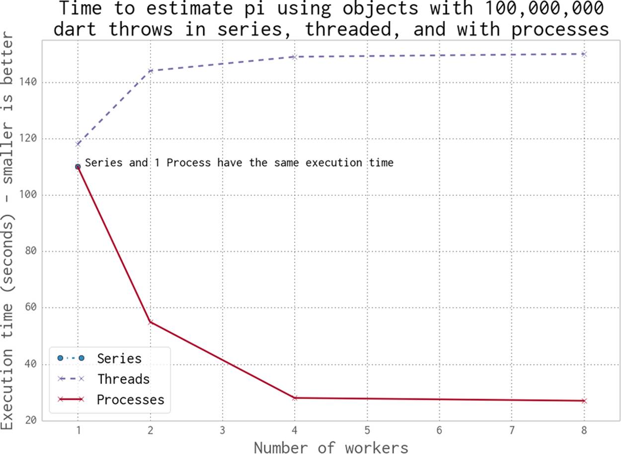
Figure 9-2. Working in series, with threads and with processes
When we use more than one thread or process, we’re asking Python to calculate the same total number of dart throws and to divide the work evenly between workers. If we want 100,000,000 dart throws in total using our Python implementation and we use two workers, then we’ll be asking both threads or both processes to generate 50,000,000 dart throws per worker.
Using one thread takes approximately 120 seconds. Using two or more threads takes longer. By using two or more processes, we make the runtime shorter. The cost of using no processes or threads (the series implementation) is the same as running with one process.
By using processes, we get a linear speedup when using two or four cores on Ian’s laptop. For the eight-worker case we’re using Intel’s Hyper-Threading Technology—the laptop only has four physical cores, so we get barely any additional speedup by running eight processes.
Example 9-1 shows the Python version of our pi estimator. If we’re using threads each instruction is bound by the GIL, so although each thread could run on a separate CPU, it will only execute when no other threads are running. The process version is not bound by this restriction, as each forked process has a private Python interpreter running as a single thread—there’s no GIL contention as no objects are shared. We use Python’s built-in random number generator, but see Random Numbers in Parallel Systems for some notes about the dangers of parallelized random number sequences.
Example 9-1. Estimating pi using a loop in Python
def estimate_nbr_points_in_quarter_circle(nbr_estimates):
nbr_trials_in_quarter_unit_circle = 0
for step inxrange(int(nbr_estimates)):
x = random.uniform(0, 1)
y = random.uniform(0, 1)
is_in_unit_circle = x * x + y * y <= 1.0
nbr_trials_in_quarter_unit_circle += is_in_unit_circle
return nbr_trials_in_quarter_unit_circle
Example 9-2 shows the __main__ block. Note that we build the Pool before we start the timer. Spawning threads is relatively instant; spawning processes involves a fork, and this takes a measurable fraction of a second. We ignore this overhead in Figure 9-2, as this cost will be a tiny fraction of the overall execution time.
Example 9-2. main for estimating pi using a loop
from multiprocessing import Pool
...
if __name__ == "__main__":
nbr_samples_in_total = 1e8
nbr_parallel_blocks = 4
pool = Pool(processes=nbr_parallel_blocks)
nbr_samples_per_worker = nbr_samples_in_total / nbr_parallel_blocks
print "Making {} samples per worker".format(nbr_samples_per_worker)
nbr_trials_per_process = [nbr_samples_per_worker] * nbr_parallel_blocks
t1 = time.time()
nbr_in_unit_circles = pool.map(calculate_pi, nbr_trials_per_process)
pi_estimate = sum(nbr_in_unit_circles) * 4 / nbr_samples_in_total
print "Estimated pi", pi_estimate
print "Delta:", time.time() - t1
We create a list containing nbr_estimates divided by the number of workers. This new argument will be sent to each worker. After execution, we’ll receive the same number of results back; we’ll sum these to estimate the number of darts in the unit circle.
We import the process-based Pool from multiprocessing. We could also have used from multiprocessing.dummy import Pool to get a threaded version—the “dummy” name is rather misleading (we confess to not understanding why it is named this way); it is simply a light wrapper around the threading module to present the same interface as the process-based Pool.
WARNING
It is worth noting that each process we create consumes some RAM from the system. You can expect a forked process using the standard libraries to take on the order of 10–20MB of RAM; if you’re using many libraries and lots of data, then you might expect each forked copy to take hundreds of megabytes. On a system with a RAM constraint, this might be a significant issue—if you run out of RAM and the system reverts to using the disk’s swap space, then any parallelization advantage will be massively lost to the slow paging of RAM back and forth to disk!
The following figures plot the average CPU utilization of Ian’s laptop’s four physical cores and their four associated hyperthreads (each hyperthread runs on unutilized silicon in a physical core). The data gathered for these figures includes the startup time of the first Python process and the cost of starting subprocesses. The CPU sampler records the entire state of the laptop, not just the CPU time used by this task.
Note that the following diagrams are created using a different timing method with a slower sampling rate than Figure 9-2, so the overall runtime is a little longer.
The execution behavior in Figure 9-3 with one process in the pool (along with the parent process) shows some overhead in the first seconds as the pool is created, and then a consistent close-to-100% CPU utilization throughout the run. With one process, we’re efficiently using one core.
Next we’ll add a second process, effectively saying Pool(processes=2). As you can see in Figure 9-4, adding a second process roughly halves the execution time to 56 seconds, and two CPUs are fully occupied. This is the best result we can expect—we’ve efficiently used all the new computing resources and we’re not losing any speed to other overheads like communication, paging to disk, or contention with competing processes that want to use the same CPUs.
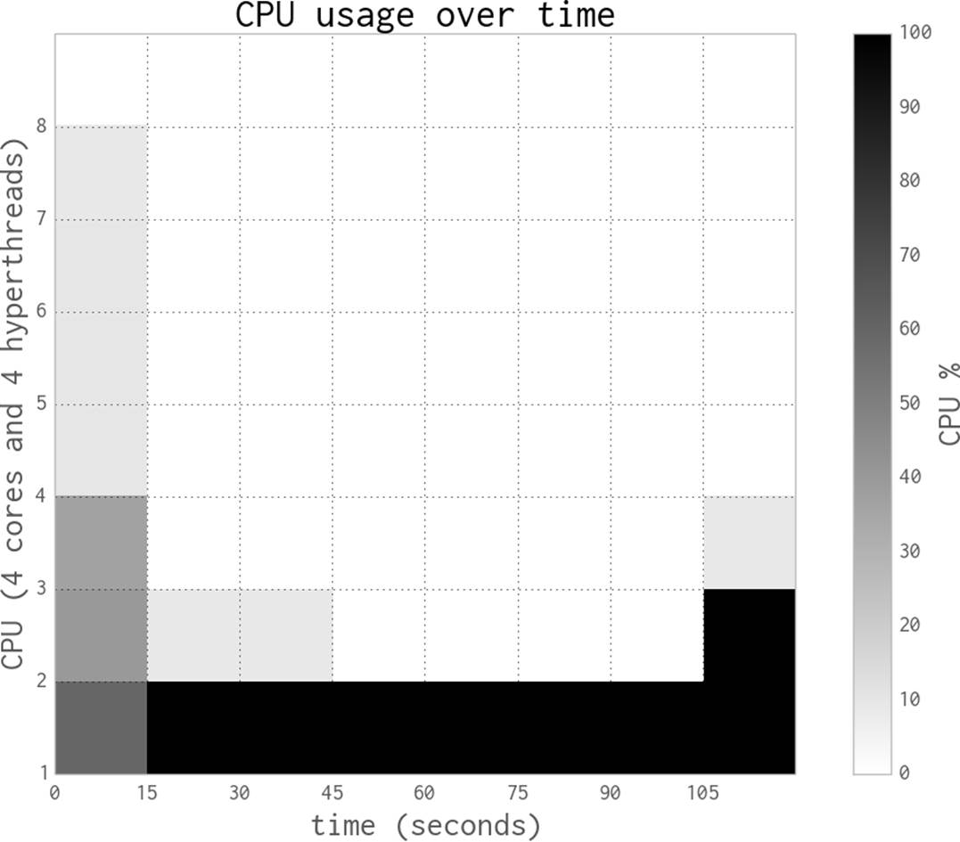
Figure 9-3. Estimating pi using Python objects and one process
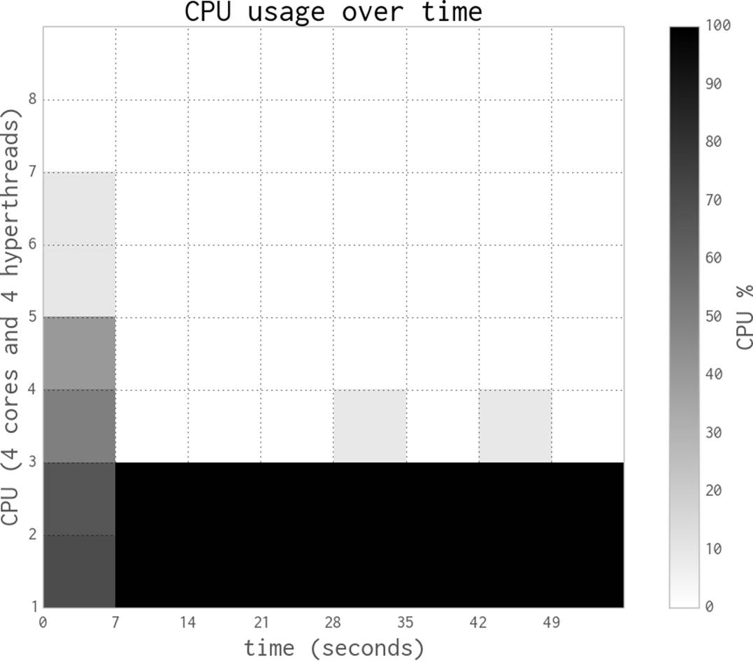
Figure 9-4. Estimating pi using Python objects and two processes
Figure 9-5 shows the results when using all four physical CPUs—now we are using all of the raw power of this laptop. Execution time is roughly a quarter that of the single-process version, at 27 seconds.
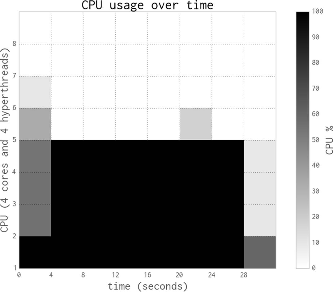
Figure 9-5. Estimating pi using Python objects and four processes
By switching to eight processes, as seen in Figure 9-6, we cannot achieve more than a tiny speedup compared to the four-process version. That is because the four hyperthreads are only able to squeeze a little extra processing power out of the spare silicon on the CPUs, and the four CPUs are already maximally utilized.
These diagrams show that we’re efficiently using more of the available CPU resources at each step, and that the HyperThread resources are a poor addition. The biggest problem when using hyperthreads is that CPython is using a lot of RAM—hyperthreading is not cache-friendly, so the spare resources on each chip are very poorly utilized. As we’ll see in the next section, numpy makes better use of these resources.
NOTE
In our experience, hyperthreading can give up to a 30% performance gain if there are enough spare computing resources. This works if, for example, you have a mix of floating-point and integer arithmetic rather than just the floating-point operations we have here. By mixing the resource requirements, the hyperthreads can schedule more of the CPU’s silicon to be working concurrently. Generally, we see hyperthreads as an added bonus and not a resource to be optimized against, as adding more CPUs is probably more economical than tuning your code (which adds a support overhead).
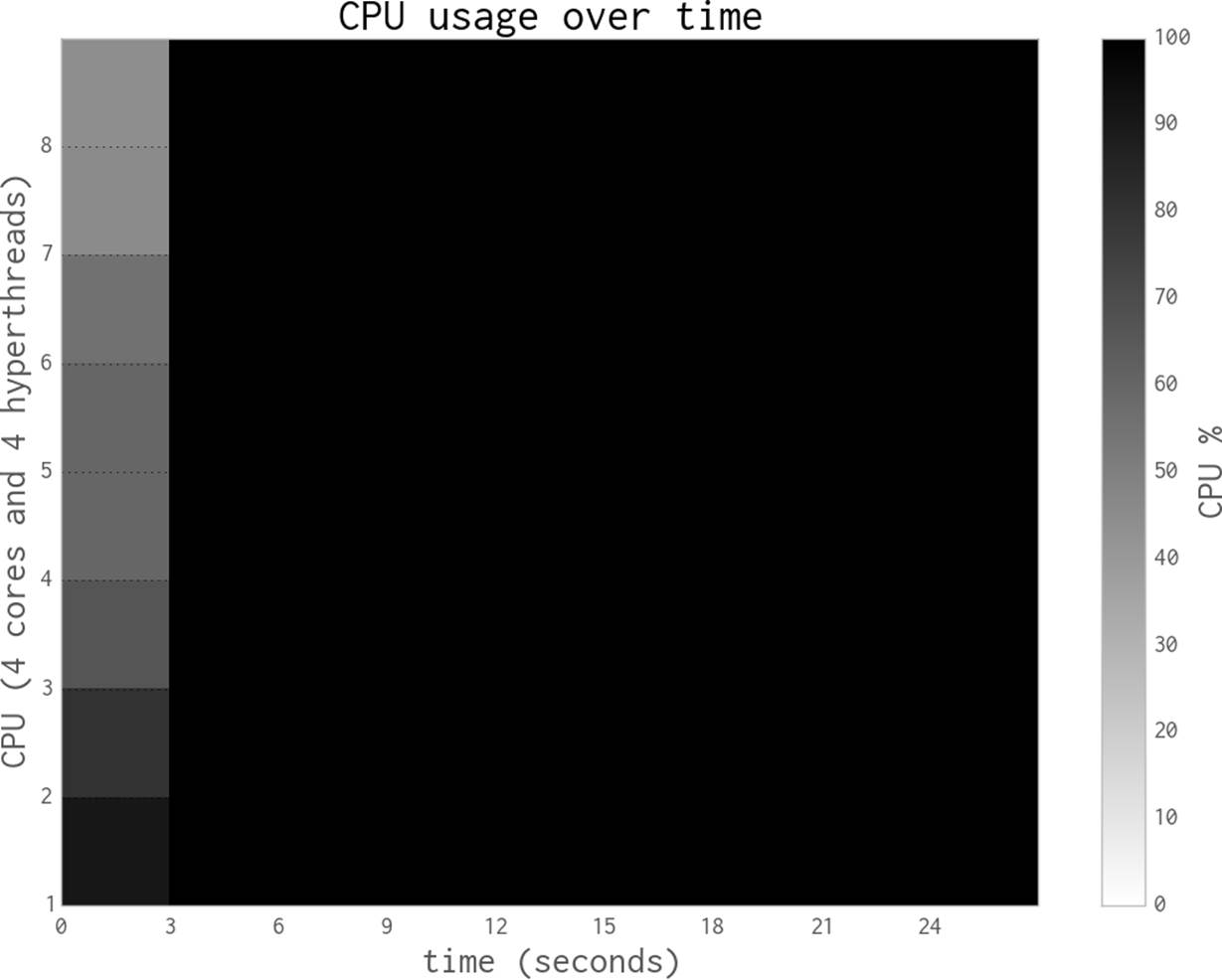
Figure 9-6. Estimating pi using Python objects and eight processes with little additional gain
Now we’ll switch to using threads in one process, rather than multiple processes. As you’ll see, the overhead caused by the “GIL battle” actually makes our code run slower.
Figure 9-7 shows two threads fighting on a dual-core system with Python 2.6 (the same effect occurs with Python 2.7)—this is the GIL battle image taken with permission from David Beazley’s blog post, “The Python GIL Visualized.” The darker red tone shows Python threads repeatedly trying to get the GIL but failing. The lighter green tone represents a running thread. White shows the brief periods when a thread is idle. We can see that there’s an overhead when adding threads to a CPU-bound task in CPython. The context-switching overhead actually adds to the overall runtime. David Beazley explains this in “Understanding the Python GIL.” Threads in Python are great for I/O-bound tasks, but they’re a poor choice for CPU-bound problems.

Figure 9-7. Python threads fighting on a dual-core machine
Each time a thread wakes up and tries to acquire the GIL (whether it is available or not), it uses some system resources. If one thread is busy, then the other will repeatedly awaken and try to acquire the GIL. These repeated attempts become expensive. David Beazley has an interactive set of plots that demonstrate the problem; you can zoom in to see every failed attempt at GIL acquisition for multiple threads on multiple CPUs. Note that this is only a problem with multiple threads running on a multicore system—a single-core system with multiple threads has no “GIL battle.” This is easily seen in the four-thread zoomable visualization on David’s site.
If the threads weren’t fighting for the GIL but were passing it back and forth efficiently, we wouldn’t expect to see any of the dark red tone; instead, we might expect the waiting thread to carry on waiting without consuming resources. Avoiding the battle for the GIL would make the overall runtime shorter, but it would still be no faster than using a single thread, due to the GIL. If there were no GIL, each thread could run in parallel without any waiting and so the threads would make use of all of the system’s resources.
It is worth noting that the negative effect of threads on CPU-bound problems is reasonably solved in Python 3.2+:
The mechanism for serializing execution of concurrently running Python threads (generally known as the GIL or Global Interpreter Lock) has been rewritten. Among the objectives were more predictable switching intervals and reduced overhead due to lock contention and the number of ensuing system calls. The notion of a “check interval” to allow thread switches has been abandoned and replaced by an absolute duration expressed in seconds.
— Raymond Hettinger
Figure 9-8 shows the results of running the same code that we used in Figure 9-5, but with threads in place of processes. Although a number of CPUs are being used, they each share the workload lightly. If each thread was running without the GIL, then we’d see 100% CPU utilization on the four CPUs. Instead, each CPU is partially utilized (due to the GIL), and in addition they are running slower than we’d like due to the GIL battle.
Compare this to Figure 9-3, where one process executes the same job in approximately 120 seconds rather than 160 seconds.
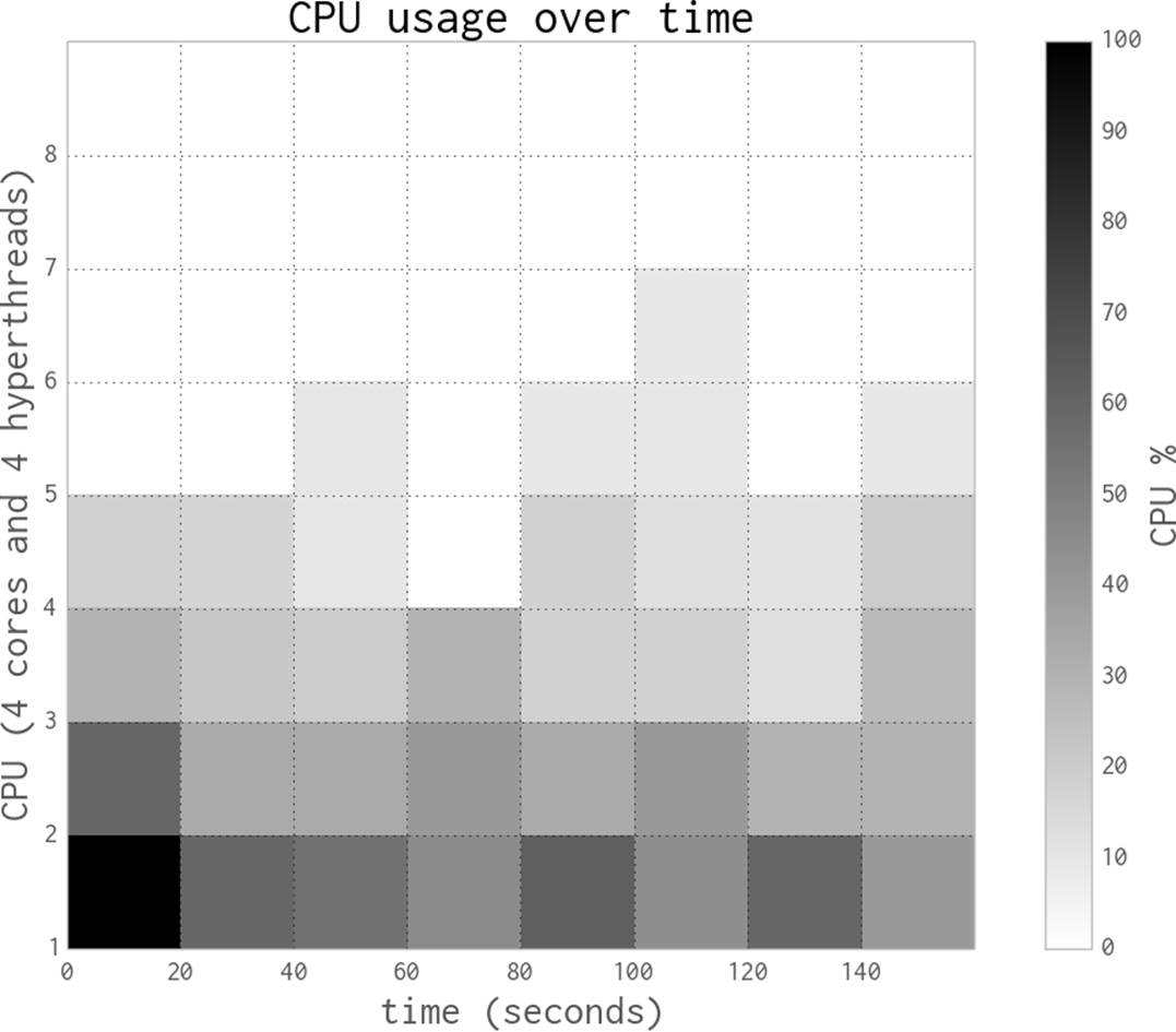
Figure 9-8. Estimating pi using Python objects and four threads
Random Numbers in Parallel Systems
Generating good random number sequences is a hard problem, and it is easy to get it wrong if you try to do it yourself. Getting a good sequence quickly in parallel is even harder—suddenly you have to worry about whether you’ll get repeating or correlated sequences in the parallel processes.
We’ve used Python’s built-in random number generator in Example 9-1, and we’ll use the numpy random number generator in the next section, in Example 9-3. In both cases the random number generators are seeded in their forked process. For the Python random example the seeding is handled internally by multiprocessing—if during a fork it sees that random is in the namespace, then it’ll force a call to seed the generators in each of the new processes.
In the forthcoming numpy example, we have to do this explicitly. If you forget to seed the random number sequence with numpy, then each of your forked processes will generate an identical sequence of random numbers.
If you care about the quality of the random numbers used in the parallel processes, we urge you to research this topic, as we don’t discuss it here. Probably the numpy and Python random number generators are good enough, but if significant outcomes depend on the quality of the random sequences (e.g., for medical or financial systems), then you must read up on this area.
Using numpy
In this section we switch to using numpy. Our dart-throwing problem is ideal for numpy vectorized operations—we generate the same estimate over 50 times faster than the previous Python examples.
The main reason that numpy is faster than pure Python when solving the same problem is that it is creating and manipulating the same object types at a very low level in contiguous blocks of RAM, rather than creating many higher-level Python objects that each require individual management and addressing.
As numpy is far more cache-friendly, we’ll also get a small speed boost when using the four hyperthreads. We didn’t get this in the pure Python version, as caches aren’t used efficiently by larger Python objects.
In Figure 9-9 we see three scenarios:
§ No use of multiprocessing (named “Series”)
§ Using threads
§ Using processes
The serial and single-worker versions execute at the same speed—there’s no overhead to using threads with numpy (and with only one worker, there’s also no gain).
When using multiple processes, we see a classic 100% utilization of each additional CPU. The result mirrors the plots shown in Figures 9-3, 9-4, 9-5, and 9-6, but the code obviously runs much faster using numpy.
Interestingly, the threaded version runs faster with more threads—this is the opposite behavior to the pure Python case, where threads made the example run slower. As discussed on the SciPy wiki, by working outside of the GIL numpy can achieve some level of additional speedup around threads.
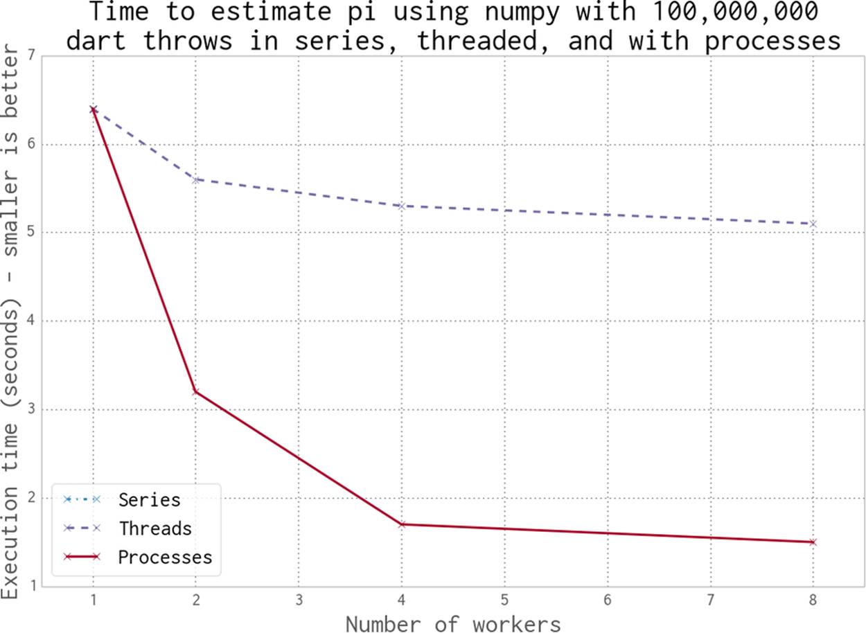
Figure 9-9. Working in series, threaded, and with processes using numpy
Using processes gives us a predictable speedup, just as it did in the pure Python example. A second CPU doubles the speed, and using four CPUs quadruples the speed.
Example 9-3 shows the vectorized form of our code. Note that the random number generator is seeded when this function is called. For the threaded version this isn’t necessary, as each thread shares the same random number generator and they access it in series. For the process version, as each new process is a fork, all the forked versions will share the same state. This means the random number calls in each will return the same sequence! Calling seed() should ensure that each of the forked processes generates a unique sequence of random numbers. Look back at Random Numbers in Parallel Systems for some notes about the dangers of parallelized random number sequences.
Example 9-3. Estimating pi using numpy
def estimate_nbr_points_in_quarter_circle(nbr_samples):
# set random seed for numpy in each new process
# else the fork will mean they all share the same state
np.random.seed()
xs = np.random.uniform(0, 1, nbr_samples)
ys = np.random.uniform(0, 1, nbr_samples)
estimate_inside_quarter_unit_circle = (xs * xs + ys * ys) <= 1
nbr_trials_in_quarter_unit_circle = np.sum(estimate_inside_quarter_unit_circle)
return nbr_trials_in_quarter_unit_circle
A short code analysis shows that the calls to random run a little slower on this machine when executed with multiple threads and the call to (xs * xs + ys * ys) <= 1 parallelizes well. Calls to the random number generator are GIL-bound as the internal state variable is a Python object.
The process to understand this was basic but reliable:
1. Comment out all of the numpy lines, and run with no threads using the serial version. Run several times and record the execution times using time.time() in __main__.
2. Add a line back (first, we added xs = np.random.uniform(...), and run several times, again recording completion times.
3. Add the next line back (now adding ys = ...), run again, and record completion time.
4. Repeat, including the nbr_trials_in_quarter_unit_circle = np.sum(...) line.
5. Repeat this process again, but this time with four threads. Repeat line by line.
6. Compare the difference in runtime at each step for no threads and four threads.
Because we’re running code in parallel, it becomes harder to use tools like line_profiler or cProfile. Recording the raw runtimes and observing the differences in behavior with different configurations takes some patience but gives solid evidence from which to draw conclusions.
NOTE
If you want to understand the serial behavior of the uniform call, take a look at the mtrand code in the numpy source and follow the call to uniform in mtrand.pyx. This is a useful exercise if you haven’t looked at the numpy source code before.
The libraries used when building numpy are important for some of the parallelization opportunities. Depending on the underlying libraries used when building numpy (e.g., whether Intel’s Math Kernel Library or OpenBLAS were included or not), you’ll see different speedup behavior.
You can check your numpy configuration using numpy.show_config(). There are some example timings on StackOverflow if you’re curious about the possibilities. Only some numpy calls will benefit from parallelization by external libraries.
Finding Prime Numbers
Next, we’ll look at testing for prime numbers over a large number range. This is a different problem to estimating pi, as the workload varies depending on your location in the number range and each individual number’s check has an unpredictable complexity. We can create a serial routine that checks for primality and then pass sets of possible factors to each process for checking. This problem is embarrassingly parallel, which means there is no state that needs to be shared.
The multiprocessing module makes it easy to control the workload, so we shall investigate how we can tune the work queue to use (and misuse!) our computing resources and explore an easy way to use our resources slightly more efficiently. This means we’ll be looking at load balancing to try to efficiently distribute our varying-complexity tasks to our fixed set of resources.
We’ll use a slightly improved algorithm from the one earlier in the book (see Idealized Computing Versus the Python Virtual Machine) that exits early if we have an even number; see Example 9-4.
Example 9-4. Finding prime numbers using Python
def check_prime(n):
if n % 2 == 0:
return False
from_i = 3
to_i = math.sqrt(n) + 1
for i inxrange(from_i, int(to_i), 2):
if n % i == 0:
return False
return True
How much variety in the workload do we see when testing for a prime with this approach? Figure 9-10 shows the increasing time cost to check for primality as the possibly-prime n increases from 10,000 to 1,000,000.
Most numbers are non-prime; they’re drawn with a dot. Some can be cheap to check for, while others require the checking of many factors. Primes are drawn with an x and form the thick darker band; they’re the most expensive to check for. The time cost of checking a number increases as nincreases, as the range of possible factors to check increases with the square root of n. The sequence of primes is not predictable, so we can’t determine the expected cost of a range of numbers (we could estimate it, but we can’t be sure of its complexity).
For the figure, we test each n 20 times and take the fastest result to remove jitter from the results.
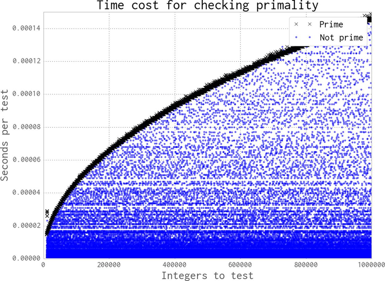
Figure 9-10. Time required to check primality as n increases
When we distribute work to a Pool of processes, we can specify how much work is passed to each worker. We could divide all of the work evenly and aim for one pass, or we could make many chunks of work and pass them out whenever a CPU is free. This is controlled using thechunksize parameter. Larger chunks of work mean less communication overhead, while smaller chunks of work mean more control over how resources are allocated.
For our prime finder, a single piece of work is a number n that is checked by check_prime. A chunksize of 10 would mean that each process handles a list of 10 integers, one list at a time.
In Figure 9-11 we can see the effect of varying the chunksize from 1 (every job is a single piece of work) to 64 (every job is a list of 64 numbers). Although having many tiny jobs gives us the greatest flexibility, it also imposes the greatest communication overhead. All four CPUs will be utilized efficiently, but the communication pipe will become a bottleneck as each job and result is passed through this single channel. If we double the chunksize to 2 our task gets solved twice as quickly, as we have less contention on the communication pipe. We might naively assume that by increasing the chunksize we will continue to improve the execution time. However, as you can see in the figure, we will again come to a point of diminishing returns.
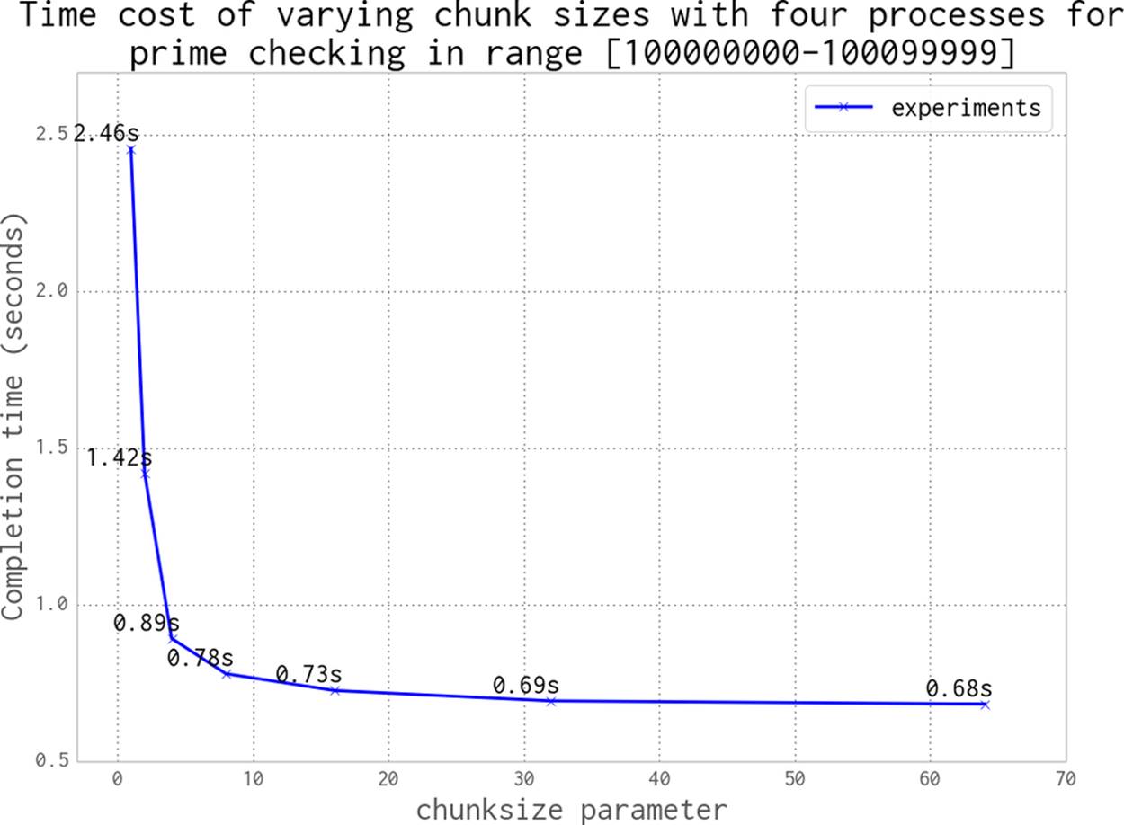
Figure 9-11. Choosing a sensible chunksize value
We can continue to increase the chunksize until we start to see a worsening of behavior. In Figure 9-12 we expand the range of chunk sizes, making them not just tiny but also huge. At the larger end of the scale the worst result shown is 1.32 seconds, where we’ve asked for chunksize to be 50000—this means our 100,000 items are divided into two work chunks, leaving two CPUs idle for that entire pass. With a chunksize of 10000 items, we are creating 10 chunks of work; this means that 4 chunks of work will run twice in parallel, followed by the 2 remaining chunks. This leaves two CPUs idle in the third round of work, which is an inefficient usage of resources.
An optimal solution in this case is to divide the total number of jobs by the number of CPUs. This is the default behavior in multiprocessing, shown as the “default” black dot in the figure.
As a general rule, the default behavior is sensible; only tune it if you expect to see a real gain, and definitely confirm your hypothesis against the default behavior.
Unlike the Monte Carlo pi problem, our prime testing calculation has varying complexity—sometimes a job exits quickly (an even number is detected the fastest), and sometimes the number is large and a prime (this takes a much longer time to check).
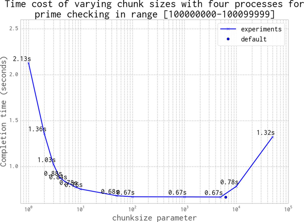
Figure 9-12. Choosing a sensible chunksize value (continued)
What happens if we randomize our job sequence? For this problem we squeeze out a 2% performance gain, as you can see in Figure 9-13. By randomizing we reduce the likelihood of the final job in the sequence taking longer than the others, leaving all but one CPU active.
As our earlier example using a chunksize of 10000 demonstrated, misaligning the workload with the number of available resources leads to inefficiency. In that case, we created three rounds of work: the first two rounds used 100% of the resources and the last round only 50%.
Figure 9-14 shows the odd effect that occurs when we misalign the number of chunks of work against the number of processors. Mismatches will underutilize the available resources. The slowest overall runtime occurs when only one chunk of work is created: this leaves three unutilized. Two work chunks leave two CPUs unutilized, and so on; only once we have four work chunks are we using all of our resources. But if we add a fifth work chunk, then again we’re underutilizing our resources—four CPUs will work on their chunks, and then one CPU will run to calculate the fifth chunk.
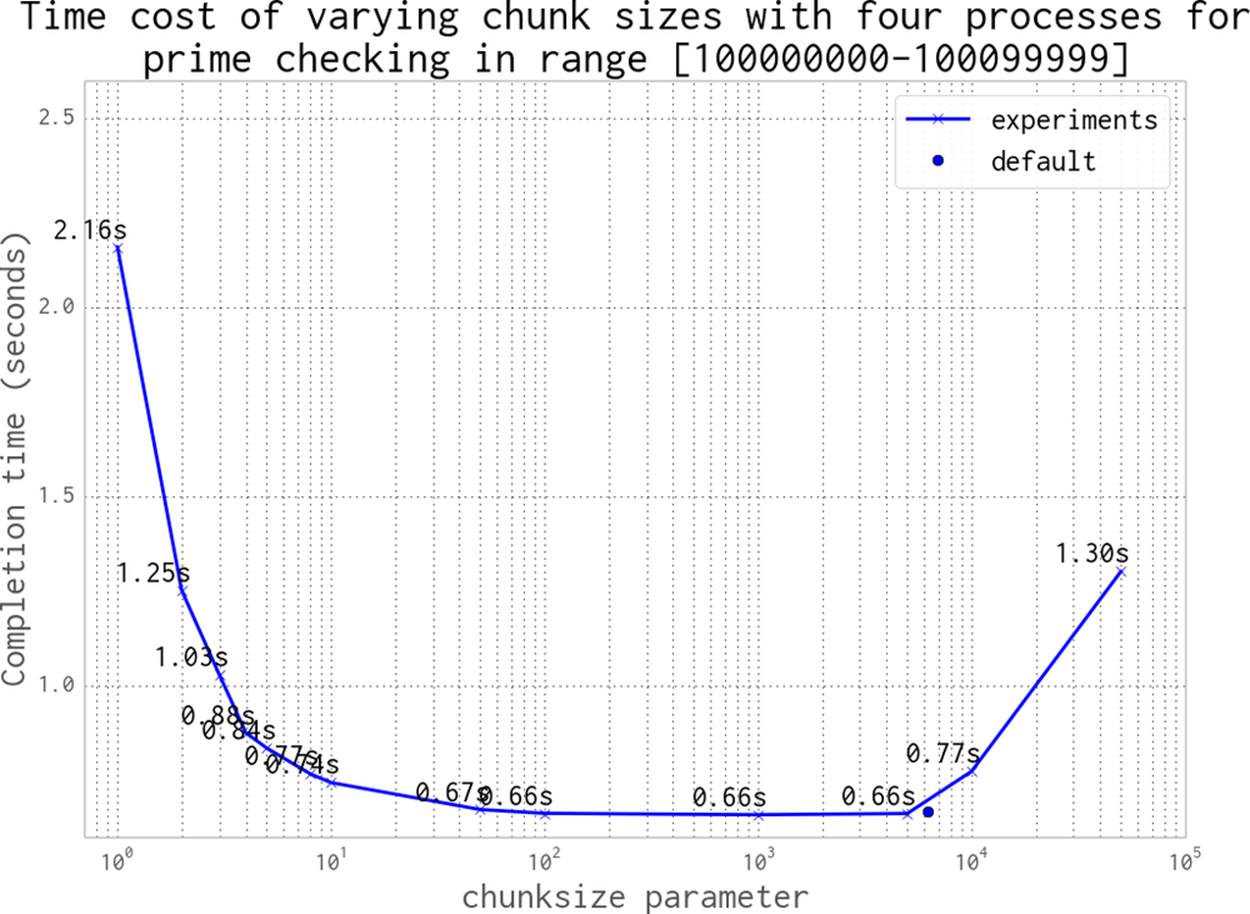
Figure 9-13. Randomizing the job sequence
As we increase the number of chunks of work, we see that the inefficiencies decrease—the difference in runtime between 29 and 32 work chunks is approximately 0.01 seconds. The general rule is to make lots of small jobs for efficient resource utilization if your jobs have varying runtimes.
Here are some strategies for efficiently using multiprocessing for embarrassingly parallel problems:
§ Split your jobs into independent units of work.
§ If your workers take varying amounts of time, then consider randomizing the sequence of work (another example would be for processing variable-sized files).
§ Sorting your work queue so slowest jobs go first may be an equally useful strategy.
§ Use the default chunksize unless you have verified reasons for adjusting it.
§ Align the number of jobs with the number of physical CPUs (again, the default chunksize takes care of this for you, although it will use any hyperthreads by default, which may not offer any additional gain).
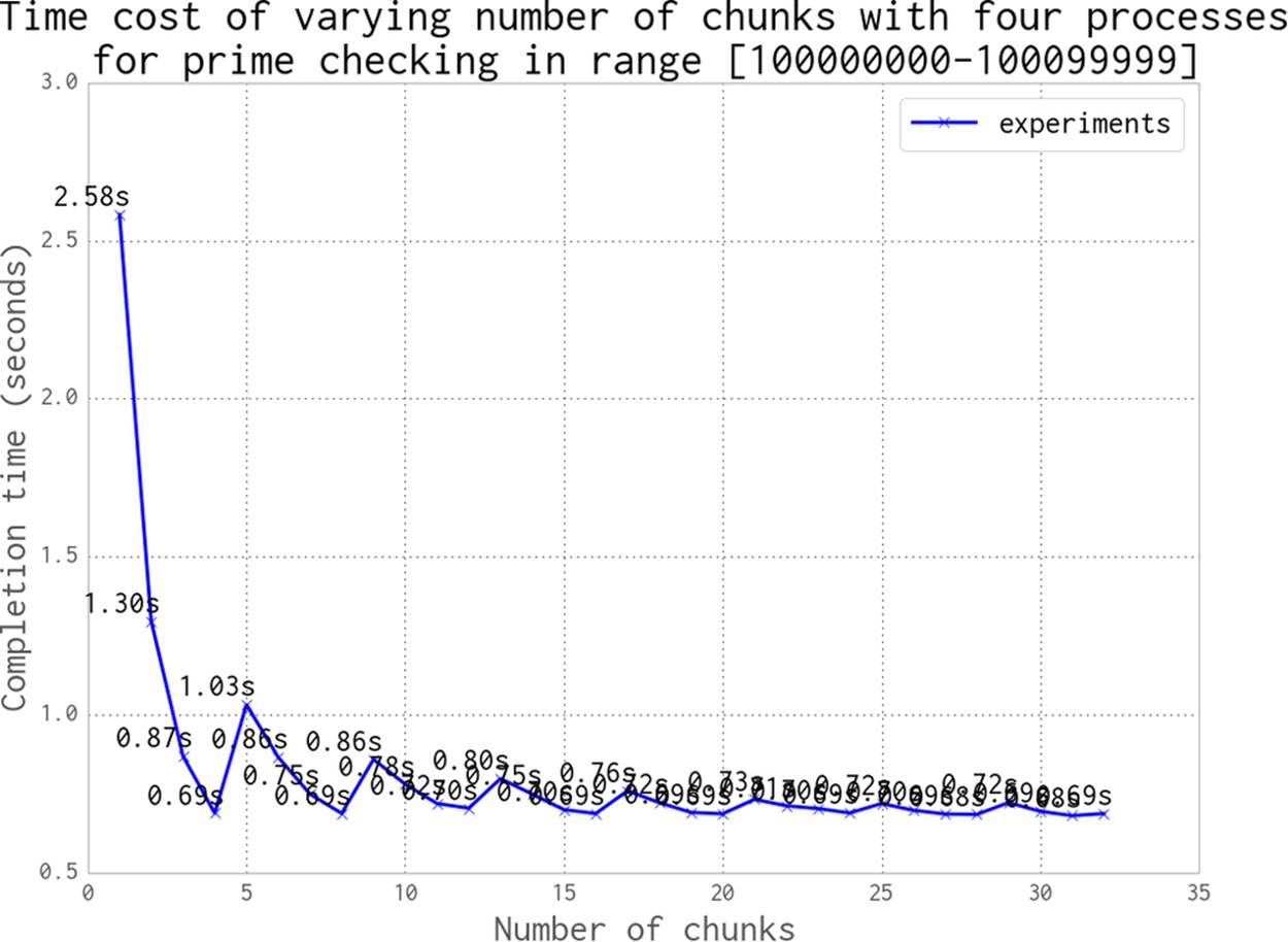
Figure 9-14. The danger of choosing an inappropriate number of chunks
Note that by default multiprocessing will see hyperthreads as additional CPUs. This means that on Ian’s laptop it will allocate eight processes when only four will really be running at 100% speed. The additional four processes could be taking up valuable RAM while barely offering any additional speed gain.
With a Pool, we can split up a chunk of predefined work up front among the available CPUs. This is less helpful if we have dynamic workloads, though, and particularly if we have workloads that arrive over time. For this sort of workload we might want to use a Queue, introduced in the next section.
NOTE
If you’re working on long-running scientific problems where each job takes many seconds (or longer) to run, then you might want to review Gael Varoquaux’s joblib. This tool supports lightweight pipelining; it sits on top of multiprocessing and offers an easier parallel interface, result caching, and debugging features.
Queues of Work
multiprocessing.Queue objects give us nonpersistent queues that can send any pickleable Python objects between processes. They carry an overhead, as each object must be pickled to be sent and then unpickled in the consumer (along with some locking operations). In the following example, we’ll see that this cost is not negligible. However, if your workers are processing larger jobs, then the communication overhead is probably acceptable.
Working with the queues is fairly easy. In this example, we’ll check for primes by consuming a list of candidate numbers and posting confirmed primes back to a definite_primes_queue. We’ll run this with one, two, four, and eight processes and confirm that all of the latter take longer than just running a single process that checks the same range.
A Queue gives us the ability to perform lots of interprocess communication using native Python objects. This can be useful if you’re passing around objects with lots of state. Since the Queue lacks persistence, though, you probably don’t want to use them for jobs that might require robustness in the face of failure (e.g., if you lose power or a hard drive gets corrupted).
Example 9-5 shows the check_prime function. We’re already familiar with the basic primality test. We run in an infinite loop, blocking (waiting until work is available) on possible_primes_queue.get() to consume an item from the queue. Only one process can get an item at a time, as the Queue object takes care of synchronizing the accesses. If there’s no work in the queue, then the .get() blocks until a task is available. When primes are found they are put back on the definite_primes_queue for consumption by the parent process.
Example 9-5. Using two Queues for IPC
FLAG_ALL_DONE = b"WORK_FINISHED"
FLAG_WORKER_FINISHED_PROCESSING = b"WORKER_FINISHED_PROCESSING"
def check_prime(possible_primes_queue, definite_primes_queue):
while True:
n = possible_primes_queue.get()
if n == FLAG_ALL_DONE:
# flag that our results have all been pushed to the results queue
definite_primes_queue.put(FLAG_WORKER_FINISHED_PROCESSING)
break
else:
if n % 2 == 0:
continue
for i inxrange(3, int(math.sqrt(n)) + 1, 2):
if n % i == 0:
break
else:
definite_primes_queue.put(n)
We define two flags: one is fed by the parent process as a poison pill to indicate that there is no more work available, while the second is fed by the worker to confirm that it has seen the poison pill and has closed itself down. The first poison pill is also known as a sentinel, as it guarantees the termination of the processing loop.
When dealing with queues of work and remote workers it can be helpful to use flags like these to record that the poison pills were sent and to check that responses were sent from the children in a sensible time window, indicating that they are shutting down. We don’t handle that process here, but adding some timekeeping is a fairly simple addition to the code. The receipt of these flags can be logged or printed during debugging.
The Queue objects are created out of a Manager in Example 9-6. We’ll use the familiar process of building a list of Process objects that each contain a forked process. The two queues are sent as arguments, and multiprocessing handles their synchronization. Having started the new processes, we hand a list of jobs to the possible_primes_queue and end with one poison pill per process. The jobs will be consumed in FIFO order, leaving the poison pills for last. In check_prime we use a blocking .get(), as the new processes will have to wait for work to appear in the queue. Since we use flags, we could add some work, deal with the results, and then iterate by adding more work, and signal the end of life of the workers by adding the poison pills later.
Example 9-6. Building two Queues for IPC
if __name__ == "__main__":
primes = []
manager = multiprocessing.Manager()
possible_primes_queue = manager.Queue()
definite_primes_queue = manager.Queue()
NBR_PROCESSES = 2
pool = Pool(processes=NBR_PROCESSES)
processes = []
for _ inrange(NBR_PROCESSES):
p = multiprocessing.Process(target=check_prime,
args=(possible_primes_queue,
definite_primes_queue))
processes.append(p)
p.start()
t1 = time.time()
number_range = xrange(100000000, 101000000)
# add jobs to the inbound work queue
for possible_prime innumber_range:
possible_primes_queue.put(possible_prime)
# add poison pills to stop the remote workers
for n inxrange(NBR_PROCESSES):
possible_primes_queue.put(FLAG_ALL_DONE)
To consume the results we start another infinite loop in Example 9-7, using a blocking .get() on the definite_primes_queue. If the finished-processing flag is found, then we take a count of the number of processes that have signaled their exit. If not, then we have a new prime and we add this to the primes list. We exit the infinite loop when all of our processes have signaled their exit.
Example 9-7. Using two Queues for IPC
processors_indicating_they_have_finished = 0
while True:
new_result = definite_primes_queue.get() # block while waiting for results
if new_result == FLAG_WORKER_FINISHED_PROCESSING:
processors_indicating_they_have_finished += 1
if processors_indicating_they_have_finished == NBR_PROCESSES:
break
else:
primes.append(new_result)
assert processors_indicating_they_have_finished == NBR_PROCESSES
print "Took:", time.time() - t1
print len(primes), primes[:10], primes[-10:]
There is quite an overhead to using a Queue, due to the pickling and synchronization. As you can see in Figure 9-15, using a Queue-less single-process solution is significantly faster than using two or more processes. The reason in this case is because our workload is very light—the communication cost dominates the overall time for this task. With Queues, two processes complete this example a little faster than one process, while four and eight processes are each slower.
If your task has a long completion time (at least a sizable fraction of a second) with a small amount of communication, then a Queue approach might be the right answer. You will have to verify whether the communication cost makes this approach useful enough.
You might wonder what happens if we remove the redundant half of the job queue (all the even numbers—these are rejected very quickly in check_prime). Halving the size of the input queue halves our execution time in each case, but it still doesn’t beat the single-process non-Queueexample! This helps to illustrate that the communication cost is the dominating factor in this problem.
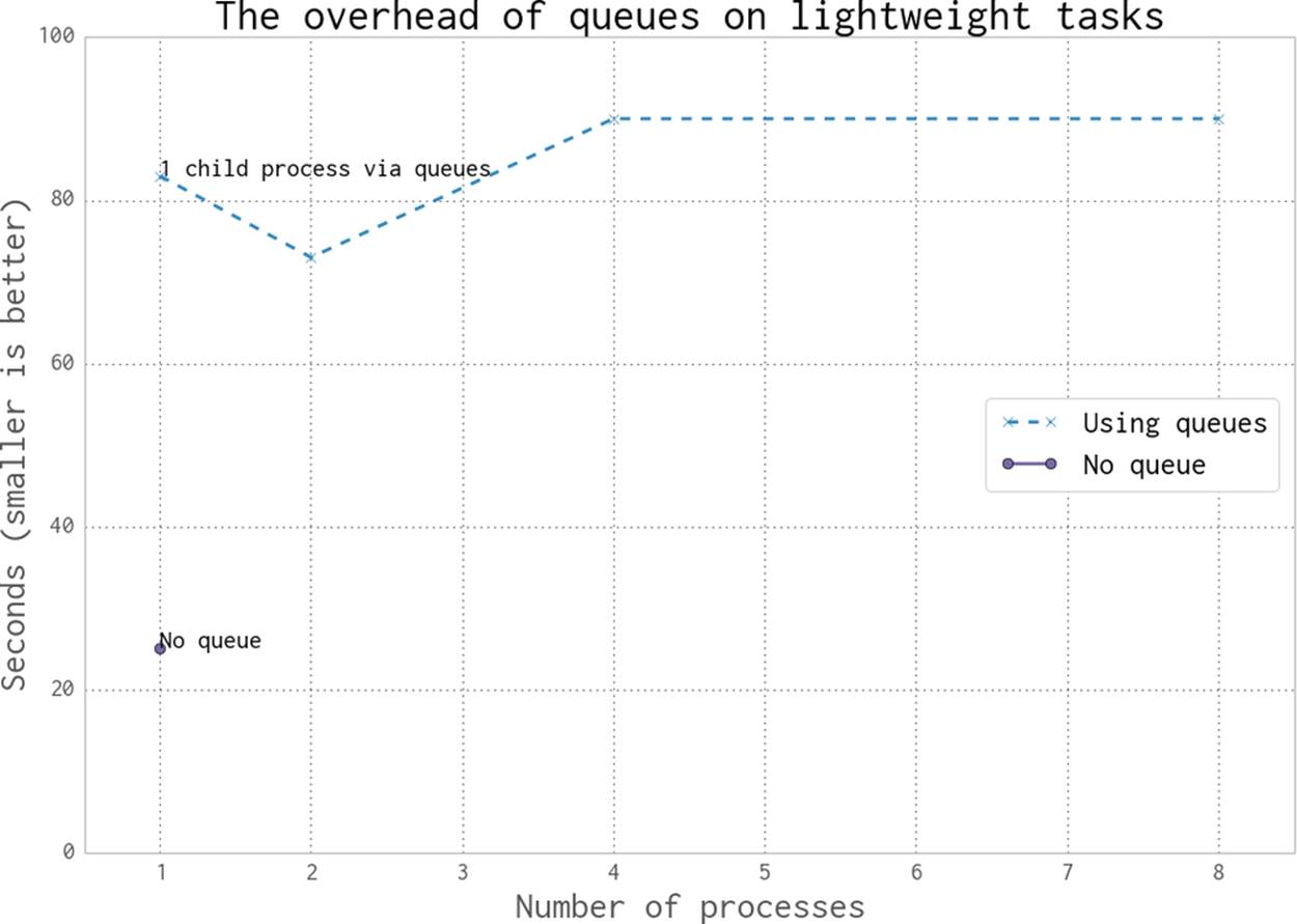
Figure 9-15. Cost of using Queue objects
Asynchronously adding jobs to the Queue
By adding a Thread into the main process, we can feed jobs asynchronously into the possible_primes_queue. In Example 9-8 we define a feed_new_jobs function: it performs the same job as the job setup routine that we had in __main__ before, but it does it in a separate thread.
Example 9-8. Asynchronous job feeding function
def feed_new_jobs(number_range, possible_primes_queue, nbr_poison_pills):
for possible_prime innumber_range:
possible_primes_queue.put(possible_prime)
# add poison pills to stop the remote workers
for n inxrange(nbr_poison_pills):
possible_primes_queue.put(FLAG_ALL_DONE)
Now, in Example 9-9, our __main__ will set up the Thread using the possible_primes_queue and then move on to the result-collection phase before any work has been issued. The asynchronous job feeder could consume work from external sources (e.g., from a database or I/O-bound communication) while the __main__ thread handles each processed result. This means that the input sequence and output sequence do not need to be created in advance; they can both be handled on the fly.
Example 9-9. Using a thread to set up an asynchronous job feeder
if __name__ == "__main__":
primes = []
manager = multiprocessing.Manager()
possible_primes_queue = manager.Queue()
...
import threading
thrd = threading.Thread(target=feed_new_jobs,
args=(number_range,
possible_primes_queue,
NBR_PROCESSES))
thrd.start()
# deal with the results
If you want robust asynchronous systems, you should almost certainly look to an external library that is mature. gevent, tornado, and Twisted are strong candidates, and Python 3.4’s tulip is a new contender. The examples we’ve looked at here will get you started, but pragmatically they are more useful for very simple systems and education than for production systems.
NOTE
Another single-machine queue you might want to investigate is PyRes. This module uses Redis (introduced in Using Redis as a Flag) to store the queue’s state. Redis is a non-Python data storage system, which means a queue of data held in Redis is readable outside of Python (so you can inspect the queue’s state) and can be shared with non-Python systems.
Be very aware that asynchronous systems require a special level of patience—you will end up tearing out your hair while you are debugging. We’d suggest:
§ Applying the “Keep It Simple, Stupid” principle
§ Avoiding asynchronous self-contained systems (like our example) if possible, as they will grow in complexity and quickly become hard to maintain
§ Using mature libraries like gevent (described in the previous chapter) that give you tried-and-tested approaches to dealing with certain problem sets
Furthermore, we strongly suggest using an external queue system (e.g., Gearman, 0MQ, Celery, PyRes, or HotQueue) that gives you external visibility on the state of the queues. This requires more thought, but is likely to save you time due to increased debug efficiency and better system visibility for production systems.
Verifying Primes Using Interprocess Communication
Prime numbers are numbers that have no factor other than themselves and 1. It stands to reason that the most common factor is 2 (every even number cannot be a prime). After that, the low prime numbers (e.g., 3, 5, 7) become common factors of larger non-primes (e.g., 9, 15, 21, respectively).
Let’s say that we’re given a large number and we’re asked to verify if it is prime. We will probably have a large space of factors to search. Figure 9-16 shows the frequency of each factor for non-primes up to 10,000,000. Low factors are far more likely to occur than high factors, but there’s no predictable pattern.

Figure 9-16. The frequency of factors of non-primes
Let’s define a new problem—suppose we have a small set of numbers and our task is to efficiently use our CPU resources to figure out if each number is a prime, one number at a time. Possibly we’ll have just one large number to test. It no longer makes sense to use one CPU to do the check; we want to coordinate the work across many CPUs.
For this section we’ll look at some larger numbers, one with 15 digits and four with 18 digits:
§ Small non-prime: 112272535095295
§ Large non-prime 1: 00109100129100369
§ Large non-prime 2: 100109100129101027
§ Prime 1: 100109100129100151
§ Prime 2: 100109100129162907
By using a smaller non-prime and some larger non-primes, we get to verify that our chosen process is not just faster at checking for primes but also is not getting slower at checking non-primes. We’ll assume that we don’t know the size or type of numbers that we’re being given, so we want the fastest possible result for all our use cases.
Cooperation comes at a cost—the cost of synchronizing data and checking the shared data can be quite high. We’ll work through several approaches here that can be used in different ways for task coordination. Note that we’re not covering the somewhat specialized message passing interface (MPI) here; we’re looking at batteries-included modules and Redis (which is very common).
If you want to use MPI, we assume you already know what you’re doing. The MPI4PY project would be a good place to start. It is an ideal technology if you want to control latency when lots of processes are collaborating, whether you have one or many machines.
For the following runs, each test is performed 20 times and the minimum time is taken to show the fastest speed that is possible for that method. In these examples we’re using various techniques to share a flag (often as 1 byte). We could use a basic object like a Lock, but then we’d only be able to share 1 bit of state. We’re choosing to show you how to share a primitive type so that more expressive state sharing is possible (even though we don’t need a more expressive state for this example).
We must emphasize that sharing state tends to make things complicated—you can easily end up in another hair-pulling state. Be careful and try to keep things as simple as they can be. It might be the case that less efficient resource usage is trumped by developer time spent on other challenges.
First we’ll discuss the results and then we’ll work through the code.
Figure 9-17 shows the first approaches to trying to use interprocess communication to test for primality faster. The benchmark is the Serial version, which does not use any interprocess communication; each attempt to speed up our code must at least be faster than this.
The Less Naive Pool version has a predictable (and good) speed. It is good enough to be rather hard to beat. Don’t overlook the obvious in your search for high-speed solutions—sometimes a dumb and good-enough solution is all you need.
The approach for the Less Naive Pool solution is to take our number under test, divide its possible-factor range evenly among the available CPUs, and then push the work out to each CPU. If any CPU finds a factor, it will exit early, but it won’t communicate this fact; the other CPUs will continue to work through their part of the range. This means for an 18-digit number (our four larger examples), the search time is the same whether it is prime or non-prime.
The Redis and Manager solutions are slower when it comes to testing a larger number of factors for primality due to the communication overhead. They use a shared flag to indicate that a factor has been found and the search should be called off.
Redis lets you share state not just with other Python processes, but also with other tools and other machines, and even to expose that state over a web-browser interface (which might be useful for remote monitoring). The Manager is a part of multiprocessing; it provides a high-level synchronized set of Python objects (including primitives, the list, and the dict).
For the larger non-prime cases, although there is a cost to checking the shared flag, this is dwarfed by the saving in search time made by signaling early that a factor has been found.
For the prime cases, though, there is no way to exit early as no factor will be found, so the cost of checking the shared flag will become the dominating cost.
Figure 9-18 shows that we can get a considerably faster result with a bit of effort. The Less Naive Pool result is still our benchmark, but the RawValue and MMap (memory-map) results are much faster than the previous Redis and Manager results. The real magic comes by taking the fastest solution and performing some less-obvious code manipulations to make a near-optimal MMap solution—this final version is faster than the Less Naive Pool solution for non-primes and almost as fast as it for primes.
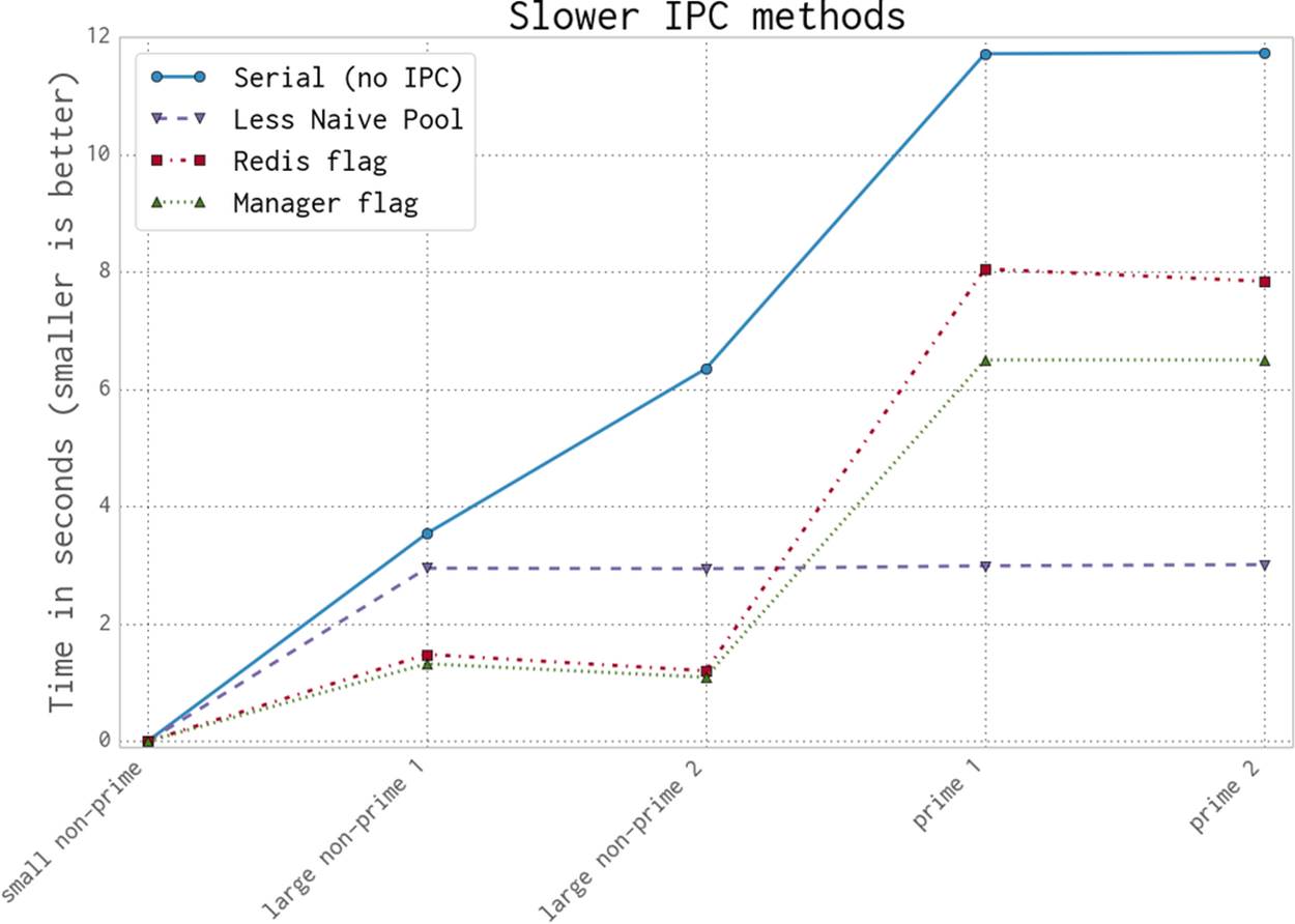
Figure 9-17. The slower ways to use IPC to validate primality
In the following sections, we’ll work through various ways of using IPC in Python to solve our cooperative search problem. We hope you’ll see that IPC is fairly easy, but generally comes with a cost.
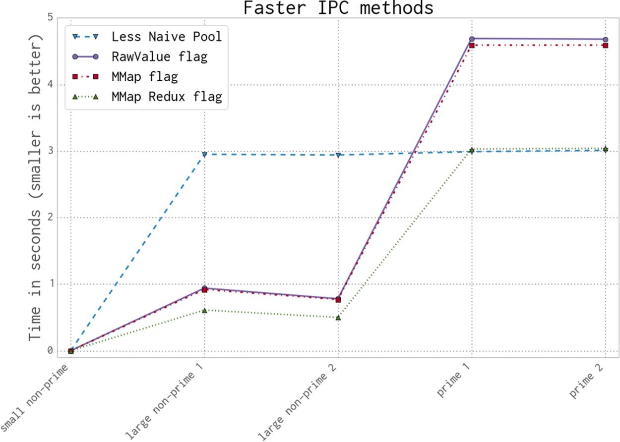
Figure 9-18. The faster ways to use IPC to validate primality
Serial Solution
We’ll start with the same serial factor-checking code that we used before, shown again in Example 9-10. As noted earlier, for any non-prime with a large factor, we could more efficiently search the space of factors in parallel. Still, a serial sweep will give us a sensible baseline to work from.
Example 9-10. Serial verification
def check_prime(n):
if n % 2 == 0:
return False
from_i = 3
to_i = math.sqrt(n) + 1
for i inxrange(from_i, int(to_i), 2):
if n % i == 0:
return False
return True
Naive Pool Solution
The Naive Pool solution works with a multiprocessing.Pool, similar to what we saw in Finding Prime Numbers and Estimating Pi Using Processes and Threads with four forked processes. We have a number to test for primality, and we divide the range of possible factors into four tuples of subranges and send these into the Pool.
In Example 9-11 we use a new method, create_range.create (which we won’t show—it’s quite boring), that splits the work space into equal-sized regions, where each item in ranges_to_check is a pair of lower and upper bounds to search between. For the first 18-digit non-prime (100109100129100369), with four processes we’ll have the factor ranges ranges_to_check == [(3, 79100057), (79100057, 158200111), (158200111, 237300165), (237300165, 316400222)] (where 316400222 is the square root of 100109100129100369 plus one). In __main__ we first establish a Pool; check_prime then splits the ranges_to_check for each possibly-prime number n via a map. If the result is False, then we have found a factor and we do not have a prime.
Example 9-11. Naive Pool solution
def check_prime(n, pool, nbr_processes):
from_i = 3
to_i = int(math.sqrt(n)) + 1
ranges_to_check = create_range.create(from_i, to_i, nbr_processes)
ranges_to_check = zip(len(ranges_to_check) * [n], ranges_to_check)
assert len(ranges_to_check) == nbr_processes
results = pool.map(check_prime_in_range, ranges_to_check)
if False inresults:
return False
return True
if __name__ == "__main__":
NBR_PROCESSES = 4
pool = Pool(processes=NBR_PROCESSES)
...
We modify the previous check_prime in Example 9-12 to take a lower and upper bound for the range to check. There’s no value in passing a complete list of possible factors to check, so we save time and memory by passing just two numbers that define our range.
Example 9-12. check_prime_in_range
def check_prime_in_range((n, (from_i, to_i))):
if n % 2 == 0:
return False
assert from_i % 2 != 0
for i inxrange(from_i, int(to_i), 2):
if n % i == 0:
return False
return True
For the “small non-prime” case the verification time via the Pool is 0.1 seconds, a significantly longer time than the original 0.000002 seconds in the Serial solution. Despite this one worse result, the overall result is a speedup across the board. We might accept that one slower result isn’t a problem—but what if we might get lots of smaller non-primes to check? It turns out we can avoid this slowdown; we’ll see that next with the Less Naive Pool solution.
A Less Naive Pool Solution
The previous solution was inefficient at validating the smaller non-prime. For any smaller (less than 18 digits) non-prime it is likely to be slower than the serial method, due to the overhead of sending out partitioned work and not knowing if a very small factor (which are the more likely factors) will be found. If a small factor is found, then the process will still have to wait for the other larger factor searches to complete.
We could start to signal between the processes that a small factor has been found, but since this happens so frequently, it will add a lot of communication overhead. The solution presented in Example 9-13 is a more pragmatic approach—a serial check is performed quickly for likely small factors, and if none are found, then a parallel search is started. Combining a serial precheck before launching a relatively more expensive parallel operation is a common approach to avoiding some of the costs of parallel computing.
Example 9-13. Improving the Naive Pool solution for the small-non-prime case
def check_prime(n, pool, nbr_processes):
# cheaply check high-probability set of possible factors
from_i = 3
to_i = 21
if notcheck_prime_in_range((n, (from_i, to_i))):
return False
# continue to check for larger factors in parallel
from_i = to_i
to_i = int(math.sqrt(n)) + 1
ranges_to_check = create_range.create(from_i, to_i, nbr_processes)
ranges_to_check = zip(len(ranges_to_check) * [n], ranges_to_check)
assert len(ranges_to_check) == nbr_processes
results = pool.map(check_prime_in_range, ranges_to_check)
if False inresults:
return False
return True
The speed of this solution is equal to or better than that of the original serial search for each of our test numbers. This is our new benchmark.
Importantly, this Pool approach gives us an optimal case for the prime-checking situation. If we have a prime, then there’s no way to exit early; we have to manually check all possible factors before we can exit.
There’s no faster way to check though these factors: any approach that adds complexity will have more instructions, so the check-all-factors case will cause the most instructions to be executed. See the various mmap solutions covered later for a discussion on how to get as close to this current result for primes as possible.
Using Manager.Value as a Flag
The multiprocessing.Manager() lets us share higher-level Python objects between processes as managed shared objects; the lower-level objects are wrapped in proxy objects. The wrapping and safety has a speed cost but also offers great flexibility. You can share both lower-level objects (e.g., integers and floats) and lists and dictionaries.
In Example 9-14 we create a Manager and then create a 1-byte (character) manager.Value(b"c", FLAG_CLEAR) flag. You could create any of the ctypes primitives (which are the same as the array.array primitives) if you wanted to share strings or numbers.
Note that FLAG_CLEAR and FLAG_SET are assigned a byte (b'0' and b'1', respectively). We chose to use the leading b to be very explicit (it might default to a Unicode or string object if left as an implicit string, depending on your environment and Python version).
Now we can flag across all of our processes that a factor has been found, so the search can be called off early. The difficulty is balancing the cost of reading the flag against the speed saving that is possible. Because the flag is synchronized, we don’t want to check it too frequently—this adds more overhead.
Example 9-14. Passing a Manager.Value object as a flag
SERIAL_CHECK_CUTOFF = 21
CHECK_EVERY = 1000
FLAG_CLEAR = b'0'
FLAG_SET = b'1'
print "CHECK_EVERY", CHECK_EVERY
if __name__ == "__main__":
NBR_PROCESSES = 4
manager = multiprocessing.Manager()
value = manager.Value(b'c', FLAG_CLEAR) # 1-byte character
...
check_prime_in_range will now be aware of the shared flag, and the routine will be checking to see if a prime has been spotted by another process. Even though we’ve yet to begin the parallel search, we must clear the flag as shown in Example 9-15 before we start the serial check. Having completed the serial check, if we haven’t found a factor, then we know that the flag must still be false.
Example 9-15. Clearing the flag with a Manager.Value
def check_prime(n, pool, nbr_processes, value):
# cheaply check high-probability set of possible factors
from_i = 3
to_i = SERIAL_CHECK_CUTOFF
value.value = FLAG_CLEAR
if notcheck_prime_in_range((n, (from_i, to_i), value)):
return False
from_i = to_i
...
How frequently should we check the shared flag? Each check has a cost, both because we’re adding more instructions to our tight inner loop and because checking requires a lock to be made on the shared variable, which adds more cost. The solution we’ve chosen is to check the flag every 1,000 iterations. Every time we check we look to see if value.value has been set to FLAG_SET, and if so, we exit the search. If in the search the process finds a factor, then it sets value.value = FLAG_SET and exits (see Example 9-16).
Example 9-16. Passing a Manager.Value object as a flag
def check_prime_in_range((n, (from_i, to_i), value)):
if n % 2 == 0:
return False
assert from_i % 2 != 0
check_every = CHECK_EVERY
for i inxrange(from_i, int(to_i), 2):
check_every -= 1
if notcheck_every:
if value.value == FLAG_SET:
return False
check_every = CHECK_EVERY
if n % i == 0:
value.value = FLAG_SET
return False
return True
The 1,000-iteration check in this code is performed using a check_every local counter. It turns out that this approach, although readable, is suboptimal for speed. By the end of this section we’ll replace it with a less readable but significantly faster approach.
You might be curious about the total number of times we check for the shared flag. In the case of the two large primes, with four processes we check for the flag 316,405 times (we check it this many times in all of the following examples). Since each check has an overhead due to locking, this cost really adds up.
Using Redis as a Flag
Redis is a key/value in-memory storage engine. It provides its own locking and each operation is atomic, so we don’t have to worry about using locks from inside Python (or from any other interfacing language).
By using Redis we make the data storage language-agnostic—any language or tool with an interface to Redis can share data in a compatible way. You could share data between Python, Ruby, C++, and PHP equally easily. You can share data on the local machine or over a network; to share to other machines all you need to do is change the Redis default of sharing only on localhost.
Redis lets you store:
§ Lists of strings
§ Sets of strings
§ Sorted sets of strings
§ Hashes of strings
Redis stores everything in RAM and snapshots to disk (optionally using journaling) and supports master/slave replication to a cluster of instances. One possibility with Redis is to use it to share a workload across a cluster, where other machines read and write state and Redis acts as a fast centralized data repository.
We can read and write a flag as a text string (all values in Redis are strings) in just the same way as we have been using Python flags previously. We create a StrictRedis interface as a global object, which talks to the external Redis server. We could create a new connection insidecheck_prime_in_range, but this is slower and can exhaust the limited number of Redis handles that are available.
We talk to the Redis server using a dictionary-like access. We can set a value using rds[SOME_KEY] = SOME_VALUE and read the string back using rds[SOME_KEY].
Example 9-17 is very similar to the previous Manager example—we’re using Redis as a substitute for the local Manager. It comes with a similar access cost. You should note that Redis supports other (more complex) data structures; it is a powerful storage engine that we’re using just to share a flag for this example. We encourage you to familiarize yourself with its features.
Example 9-17. Using an external Redis server for our flag
FLAG_NAME = b'redis_primes_flag'
FLAG_CLEAR = b'0'
FLAG_SET = b'1'
rds = redis.StrictRedis()
def check_prime_in_range((n, (from_i, to_i))):
if n % 2 == 0:
return False
assert from_i % 2 != 0
check_every = CHECK_EVERY
for i inxrange(from_i, int(to_i), 2):
check_every -= 1
if notcheck_every:
flag = rds[FLAG_NAME]
if flag == FLAG_SET:
return False
check_every = CHECK_EVERY
if n % i == 0:
rds[FLAG_NAME] = FLAG_SET
return False
return True
def check_prime(n, pool, nbr_processes):
# cheaply check high-probability set of possible factors
from_i = 3
to_i = SERIAL_CHECK_CUTOFF
rds[FLAG_NAME] = FLAG_CLEAR
if notcheck_prime_in_range((n, (from_i, to_i))):
return False
...
if False inresults:
return False
return True
To confirm that the data is stored outside of these Python instances, we can invoke redis-cli at the command line, as in Example 9-18, and get the value stored in the key redis_primes_flag. You’ll note that the returned item is a string (not an integer). All values returned from Redis are strings, so if you want to manipulate them in Python, you’ll have to convert them to an appropriate datatype first.
Example 9-18. redis-cli example
$ redis-cli
redis 127.0.0.1:6379> GET "redis_primes_flag"
"0"
One powerful argument in favor of the use of Redis for data sharing is that it lives outside of the Python world—non-Python developers on your team will understand it, and many tools exist for it. They’ll be able to look at its state while reading (but not necessarily running and debugging) your code and follow what’s happening. From a team-velocity perspective this might be a big win for you, despite the communication overhead of using Redis. Whilst Redis is an additional dependency on your project, you should note that it is a very commonly deployed tool, and is well debugged and well understood. Consider it a powerful tool to add to your armory.
Redis has many configuration options. By default it uses a TCP interface (that’s what we’re using), although the benchmark documentation notes that sockets might be much faster. It also states that while TCP/IP lets you share data over a network between different types of OS, other configuration options are likely to be faster (but also to limit your communication options):
When the server and client benchmark programs run on the same box, both the TCP/IP loopback and unix domain sockets can be used. It depends on the platform, but unix domain sockets can achieve around 50% more throughput than the TCP/IP loopback (on Linux for instance). The default behavior of redis-benchmark is to use the TCP/IP loopback. The performance benefit of unix domain sockets compared to TCP/IP loopback tends to decrease when pipelining is heavily used (i.e. long pipelines).
— Redis documentation
Using RawValue as a Flag
multiprocessing.RawValue is a thin wrapper around a ctypes block of bytes. It lacks synchronization primitives, so there’s little to get in our way in our search for the fastest way to set a flag between processes. It will be almost as fast as the following mmap example (it is only slower because a few more instructions get in the way).
Again, we could use any ctypes primitive; there’s also a RawArray option for sharing an array of primitive objects (which will behave similarly to array.array). RawValue avoids any locking—it is faster to use, but you don’t get atomic operations.
Generally, if you avoid the synchronization that Python provides during IPC, you’ll come unstuck (once again, back to that pulling-your-hair-out situation). However, in this problem it doesn’t matter if one or more processes set the flag at the same time—the flag only gets switched in one direction, and every other time it is read it is just to learn if the search can be called off.
Because we never reset the state of the flag during the parallel search, we don’t need synchronization. Be aware that this may not apply to your problem. If you avoid synchronization, please make sure you are doing it for the right reasons.
If you want to do things like update a shared counter, look at the documentation for the Value and use a context manager with value.get_lock(), as the implicit locking on a Value doesn’t allow for atomic operations.
This example looks very similar to the previous Manager example. The only difference is that in Example 9-19 we create the RawValue as a 1-character (byte) flag.
Example 9-19. Creating and passing a RawValue
if __name__ == "__main__":
NBR_PROCESSES = 4
value = multiprocessing.RawValue(b'c', FLAG_CLEAR) # 1-byte character
pool = Pool(processes=NBR_PROCESSES)
...
The flexibility to use managed and raw values is a benefit of the clean design for data sharing in multiprocessing.
Using mmap as a Flag
Finally, we get to the fastest way of sharing bytes. Example 9-20 shows a memory-mapped (shared memory) solution using the mmap module. The bytes in a shared memory block are not synchronized, and they come with very little overhead. They act like a file—in this case, they are a block of memory with a file-like interface. We have to seek to a location and read or write sequentially. Typically mmap is used to give a short (memory-mapped) view into a larger file, but in our case, rather than specifying a file number as the first argument, we instead pass -1 to indicate that we want an anonymous block of memory. We could also specify whether we want read-only or write-only access (we want both, which is the default).
Example 9-20. Using a shared memory flag via mmap
sh_mem = mmap.mmap(-1, 1) # memory map 1 byte as a flag
def check_prime_in_range((n, (from_i, to_i))):
if n % 2 == 0:
return False
assert from_i % 2 != 0
check_every = CHECK_EVERY
for i inxrange(from_i, int(to_i), 2):
check_every -= 1
if notcheck_every:
sh_mem.seek(0)
flag = sh_mem.read_byte()
if flag == FLAG_SET:
return False
check_every = CHECK_EVERY
if n % i == 0:
sh_mem.seek(0)
sh_mem.write_byte(FLAG_SET)
return False
return True
def check_prime(n, pool, nbr_processes):
# cheaply check high-probability set of possible factors
from_i = 3
to_i = SERIAL_CHECK_CUTOFF
sh_mem.seek(0)
sh_mem.write_byte(FLAG_CLEAR)
if notcheck_prime_in_range((n, (from_i, to_i))):
return False
...
if False inresults:
return False
return True
mmap supports a number of methods that can be used to move around in the file that it represents (including find, readline, and write). We are using it in the most basic way—we seek to the start of the memory block before each read or write and, since we’re sharing just 1 byte, we useread_byte and write_byte to be explict.
There is no Python overhead for locking and no interpretation of the data; we’re dealing with bytes directly with the operating system, so this is our fastest communication method.
Using mmap as a Flag Redux
While the previous mmap result was the best overall, we couldn’t help but think that we should be able to get back to the Naive Pool result for the most expensive case of having primes. The goal is to accept that there is no early exit from the inner loop and to minimize the cost of anything extraneous.
This section presents a slightly more complex solution. The same changes can be made to the other flag-based approaches we’ve seen, although this mmap result will still be fastest.
In our previous examples, we’ve used CHECK_EVERY. This means we have the check_next local variable to track, decrement, and use in Boolean tests—and each operation adds a bit of extra time to every iteration. In the case of validating a large prime, this extra management overhead occurs over 300,000 times.
The first optimization, shown in Example 9-21, is to realize that we can replace the decremented counter with a look-ahead value, and then we only have to do a Boolean comparison on the inner loop. This removes a decrement, which, due to Python’s interpreted style, is quite slow. This optimization works in this test in CPython 2.7, but it is unlikely to offer any benefit in a smarter compiler (e.g., PyPy or Cython). This step saved 0.7 seconds when checking one of our large primes.
Example 9-21. Starting to optimize away our expensive logic
def check_prime_in_range((n, (from_i, to_i))):
if n % 2 == 0:
return False
assert from_i % 2 != 0
check_next = from_i + CHECK_EVERY
for i inxrange(from_i, int(to_i), 2):
if check_next == i:
sh_mem.seek(0)
flag = sh_mem.read_byte()
if flag == FLAG_SET:
return False
check_next += CHECK_EVERY
if n % i == 0:
sh_mem.seek(0)
sh_mem.write_byte(FLAG_SET)
return False
return True
We can also entirely replace the logic that the counter represents, as shown in Example 9-22, by unrolling our loop into a two-stage process. First, the outer loop covers the expected range, but in steps, on CHECK_EVERY. Second, a new inner loop replaces the check_every logic—it checks the local range of factors and then finishes. This is equivalent to the if not check_every: test. We follow this with the previous sh_mem logic to check the early-exit flag.
Example 9-22. Optimizing away our expensive logic
def check_prime_in_range((n, (from_i, to_i))):
if n % 2 == 0:
return False
assert from_i % 2 != 0
for outer_counter inxrange(from_i, int(to_i), CHECK_EVERY):
upper_bound = min(int(to_i), outer_counter + CHECK_EVERY)
for i inxrange(outer_counter, upper_bound, 2):
if n % i == 0:
sh_mem.seek(0)
sh_mem.write_byte(FLAG_SET)
return False
sh_mem.seek(0)
flag = sh_mem.read_byte()
if flag == FLAG_SET:
return False
return True
The speed impact is dramatic. Our non-prime case improves even further, but more importantly, our prime-checking case is very nearly as fast as the Less Naive Pool version (it is now just 0.05 seconds slower). Given that we’re doing a lot of extra work with interprocess communication, this is a very interesting result. Do note, though, that it is specific to CPython and unlikely to offer any gains when run through a compiler.
We can go even further (but frankly, this is a bit foolish). Lookups for variables that aren’t declared in the local scope are a little expensive. We can create local references to the global FLAG_SET and the frequently used .seek() and .read_byte() methods to avoid their more expensive lookups. The resulting code (Example 9-23) is even less readable than before, though, and we really recommend that you do not do this. This final result is 1.5% slower than the Less Naive Pool version when checking the larger primes. Given that we’re 4.8x faster for the non-prime cases, we’ve probably taken this example about as far as it can (and should!) go.
Example 9-23. Breaking the “don’t hurt team velocity” rule to eke out an extra speedup
def check_prime_in_range((n, (from_i, to_i))):
if n % 2 == 0:
return False
assert from_i % 2 != 0
FLAG_SET_LOCAL = FLAG_SET
sh_seek = sh_mem.seek
sh_read_byte = sh_mem.read_byte
for outer_counter inxrange(from_i, int(to_i), CHECK_EVERY):
upper_bound = min(int(to_i), outer_counter + CHECK_EVERY)
for i inxrange(outer_counter, upper_bound, 2):
if n % i == 0:
sh_seek(0)
sh_mem.write_byte(FLAG_SET)
return False
sh_seek(0)
if sh_read_byte() == FLAG_SET_LOCAL:
return False
return True
This behavior, with manual loop unrolling and creating local references to global objects, is foolish. Overall, it is bound to lower team velocity by making the code harder to understand, and really this is the job of a compiler (e.g., a JIT compiler like PyPy or a static compiler like Cython).
Humans shouldn’t be doing this sort of manipulation, because it’ll be very brittle. We haven’t tested this optimization approach in Python 3+, and we don’t want to—we don’t really expect that these incremental improvements will work in another version of Python (and certainly not in a different implementation, like PyPy or IronPython).
We’re showing you so you know that it might be possible, and warning you that to keep your sanity you really should let compilers take care of this sort of work for you.
Sharing numpy Data with multiprocessing
When working with large numpy arrays, you’re bound to wonder if you can share the data for read and write access, without a copy, between processes. It is possible, though a little fiddly. We’d like to acknowledge StackOverflow user pv for the inspiration for this demo.[25]
WARNING
Do not use this method to re-create the behaviors of BLAS, MKL, Accelerate, and ATLAS. These libraries all have multithreading support in their primitives, and it is likely that they are better-debugged than any new routine that you create. They can require some configuration to enable multithreading support, but it would be wise to see if these libraries can give you free speedups before you invest time (and lose time to debugging!) writing your own.
Sharing a large matrix between processes has several benefits:
§ Only one copy means no wasted RAM.
§ No time is wasted copying large blocks of RAM.
§ You gain the possibility of sharing partial results between the processes.
Thinking back to the pi estimation demo using numpy in Using numpy, we had the problem that the random number generation was a serial process. Here we can imagine forking processes that share one large array, each one using a differently seeded random number generator to fill in a section of the array with random numbers, and therefore completing the generation of a large random block faster than is possible with a single process.
To verify this, we modified the forthcoming demo to create a large random matrix (10,000 by 80,000 elements) as a serial process and by splitting the matrix into four segments where random is called in parallel (in both cases, one row at a time). The serial process took 15 seconds, and the parallel version took 4 seconds. Refer back to Random Numbers in Parallel Systems to understand some of the dangers of parallelized random number generation.
For the rest of this section we’ll use a simplified demo that illustrates the point while remaining easy to verify.
In Figure 9-19 you can see the output from htop on Ian’s laptop. It shows four child processes of the parent (with PID 11268), where all five processes are sharing a single 10,000 × 80,000-element numpy array of doubles. One copy of this array costs 6.4 GB, and the laptop only has 8 GB—you can see in htop by the process meters that the Mem reading shows a maximum of 7,941 MB RAM.
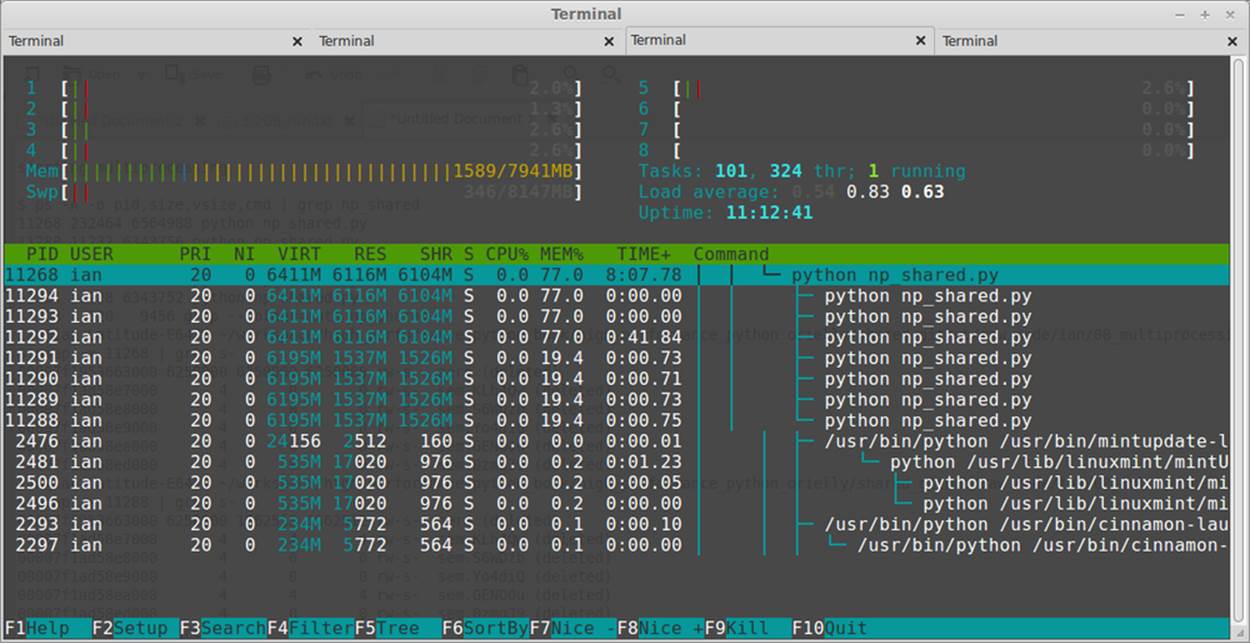
Figure 9-19. htop showing RAM and swap usage
To understand this demo, we’ll first walk through the console output, and then we’ll look at the code. In Example 9-24, we start the parent process: it allocates a 6.4 GB double array of dimensions 10,000 × 80,000, filled with the value zero. The 10,000 rows will be passed out as indices to the worker function, and the worker will operate on each column of 80,000 items in turn. Having allocated the array, we fill it with the answer to life, the universe, and everything (42!). We can test in the worker function that we’re receiving this modified array and not a filled-with-0s version to confirm that this code is behaving as expected.
Example 9-24. Setting up the shared array
$ python np_shared.py
Created shared array with 6,400,000,000 nbytes
Shared array id is 20255664 in PID 11268
Starting with an array of 0 values:
[[ 0. 0. 0. ..., 0. 0. 0.]
...,
[ 0. 0. 0. ..., 0. 0. 0.]]
Original array filled with value 42:
[[ 42. 42. 42. ..., 42. 42. 42.]
...,
[ 42. 42. 42. ..., 42. 42. 42.]]
Press a key to start workers using multiprocessing...
In Example 9-25, we’ve started four processes working on this shared array. No copy of the array was made; each process is looking at the same large block of memory and each process has a different set of indices to work from. Every few thousand lines the worker outputs the current index and its PID, so we can observe its behavior. The worker’s job is trivial—it will check that the current element is still set to the default (so we know that no other process has modified it already), and then it will overwrite this value with the current PID. Once the workers have completed, we return to the parent process and print the array again. This time, we see that it is filled with PIDs rather than 42.
Example 9-25. Running worker_fn on the shared array
worker_fn: with idx 0
id of shared_array is 20255664 in PID 11288
worker_fn: with idx 2000
id of shared_array is 20255664 in PID 11291
worker_fn: with idx 1000
id of shared_array is 20255664 in PID 11289
...
worker_fn: with idx 8000
id of shared_array is 20255664 in PID 11290
The default value has been over-written with worker_fn's result:
[[ 11288. 11288. 11288. ..., 11288. 11288. 11288.]
...,
[ 11291. 11291. 11291. ..., 11291. 11291. 11291.]]
Finally, in Example 9-26 we use a Counter to confirm the frequency of each PID in the array. As the work was evenly divided, we expect to see each of the four PIDs represented an equal number of times. In our 800,000,000-element array, we see four sets of 200,000,000 PIDs. The table output is presented using PrettyTable.
Example 9-26. Verifying the result on the shared array
Verification - extracting unique values from 800,000,000 items
in the numpy array (this might be slow)...
Unique values in shared_array:
+---------+-----------+
| PID | Count |
+---------+-----------+
| 11288.0 | 200000000 |
| 11289.0 | 200000000 |
| 11290.0 | 200000000 |
| 11291.0 | 200000000 |
+---------+-----------+
Press a key to exit...
Having completed, the program now exits, and the array is deleted.
We can take a peek inside each process under Linux using ps and pmap. Example 9-27 shows the result of calling ps. Breaking apart this command line:
§ ps tells us about the process.
§ -A lists all processes.
§ -o pid,size,vsize,cmd outputs the PID, size information, and the command name.
§ grep is used to filter all other results and leave only the lines for our demo.
The parent process (PID 11268) and its four forked children are shown in the output. The result is similar to what we saw in htop. We can use pmap to look at the memory map of each process, requesting extended output with -x. We grep for the pattern s- to list blocks of memory that are marked as being shared. In the parent process and the child processes, we see a 6,250,000 KB (6.2 GB) block that is shared between them.
Example 9-27. Using pmap and ps to investigate the operating system’s view of the processes
$ ps -A -o pid,size,vsize,cmd | grep np_shared
11268 232464 6564988 python np_shared.py
11288 11232 6343756 python np_shared.py
11289 11228 6343752 python np_shared.py
11290 11228 6343752 python np_shared.py
11291 11228 6343752 python np_shared.py
ian@ian-Latitude-E6420 $ pmap -x 11268 | grep s-
Address Kbytes RSS Dirty Mode Mapping
00007f1953663000 6250000 6250000 6250000 rw-s- zero (deleted)
...
ian@ian-Latitude-E6420 $ pmap -x 11288 | grep s-
Address Kbytes RSS Dirty Mode Mapping
00007f1953663000 6250000 1562512 1562512 rw-s- zero (deleted)
...
Example 9-28 shows the important steps taken to share this array. We use a multprocessing.Array to allocate a shared block of memory as a 1D array. We then instantiate a numpy array from this object and reshape it back to a 2D array. Now we have a numpy-wrapped block of memory that can be shared between processes and addressed as though it were a normal numpy array. numpy is not managing the RAM; multiprocessing.Array is managing it.
Example 9-28. Sharing the numpy array using multiprocessing
import os
import multiprocessing
from collections import Counter
import ctypes
import numpy as np
from prettytable import PrettyTable
SIZE_A, SIZE_B = 10000, 80000 # 6.2GB - starts to use swap (maximal RAM usage)
In Example 9-29, you can see that each forked process has access to a global main_nparray. While the forked process has a copy of the numpy object, the underlying bytes that the object accesses are stored as shared memory. Our worker_fn will overwrite a chosen row (via idx) with the current process identifier.
Example 9-29. worker_fn for sharing numpy arrays using multiprocessing
def worker_fn(idx):
"""Do some work on the shared np array on row idx"""
# confirm that no other process has modified this value already
assert main_nparray[idx, 0] == DEFAULT_VALUE
# inside the subprocess print the PID and id of the array
# to check we don't have a copy
if idx % 1000 == 0:
print " {}: with idx {}\n id of local_nparray_in_process is {} in PID {}"\
.format(worker_fn.__name__, idx, id(main_nparray), os.getpid())
# we can do any work on the array; here we set every item in this row to
# have the value of the process ID for this process
main_nparray[idx, :] = os.getpid()
In our __main__ in Example 9-30, we’ll work through three major stages:
1. Build a shared multiprocessing.Array and convert it into a numpy array.
2. Set a default value into the array, and spawn four processes to work on the array in parallel.
3. Verify the array’s contents after the processes return.
Typically, you’d set up a numpy array and work on it in a single process, probably doing something like arr = np.array((100, 5), dtype=np.float_). This is fine in a single process, but you can’t share this data across processes for both reading and writing.
The trick is to make a shared block of bytes. One way is to create a multiprocessing.Array. By default the Array is wrapped in a lock to prevent concurrent edits, but we don’t need this lock as we’ll be careful about our access patterns. To communicate this clearly to other team members, it is worth being explicit and setting lock=False.
If you don’t set lock=False, then you’ll have an object rather than a reference to the bytes, and you’ll need to call .get_obj() to get to the bytes. By calling .get_obj() you bypass the lock, so there’s no value in not being explicit about this in the first place.
Next, we take this block of shareable bytes and wrap a numpy array around them using frombuffer. The dtype is optional, but since we’re passing bytes around it is always sensible to be explicit. We reshape so we can address the bytes as a 2D array. By default the array values are set to 0. Example 9-30 shows our __main__ in full.
Example 9-30. main to set up numpy arrays for sharing
if __name__ == '__main__':
DEFAULT_VALUE = 42
NBR_OF_PROCESSES = 4
# create a block of bytes, reshape into a local numpy array
NBR_ITEMS_IN_ARRAY = SIZE_A * SIZE_B
shared_array_base = multiprocessing.Array(ctypes.c_double,
NBR_ITEMS_IN_ARRAY, lock=False)
main_nparray = np.frombuffer(shared_array_base, dtype=ctypes.c_double)
main_nparray = main_nparray.reshape(SIZE_A, SIZE_B)
# assert no copy was made
assert main_nparray.base.base isshared_array_base
print "Created shared array with {:,} nbytes".format(main_nparray.nbytes)
print "Shared array id is {} in PID {}".format(id(main_nparray), os.getpid())
print "Starting with an array of 0 values:"
print main_nparray
To confirm that our processes are operating on the same block of data that we started with, we’ll set each item to a new DEFAULT_VALUE—Syou’ll see that at the top of Example 9-31 (we use the answer to life, the universe, and everything). Next, we build a Pool of processes (four in this case) and then send batches of row indices via the call to map.
Example 9-31. main for sharing numpy arrays using multiprocessing
# modify the data via our local numpy array
main_nparray.fill(DEFAULT_VALUE)
print "Original array filled with value {}:".format(DEFAULT_VALUE)
print main_nparray
raw_input("Press a key to start workers using multiprocessing...")
# create a pool of processes that will share the memory block
# of the global numpy array, and share the reference to the underlying
# block of data so we can build a numpy array wrapper in the new processes
pool = multiprocessing.Pool(processes=NBR_OF_PROCESSES)
# perform a map where each row index is passed as a parameter to the
# worker_fn
pool.map(worker_fn, xrange(SIZE_A))
Once we’ve completed the parallel processing, we return to the parent process to verify the result (Example 9-32). The verification step runs through a flattened view on the array (note that the view does not make a copy; it just creates a 1D iterable view on the 2D array), counting the frequency of each PID. Finally, we perform some assert checks to make sure we have the expected counts.
Example 9-32. main to verify the shared result
print "Verification - extracting unique values from {:,} items\nin the numpy
array (this might be slow)...".format(NBR_ITEMS_IN_ARRAY)
# main_nparray.flat iterates over the contents of the array, it doesn't
# make a copy
counter = Counter(main_nparray.flat)
print "Unique values in main_nparray:"
tbl = PrettyTable(["PID", "Count"])
for pid, count incounter.items():
tbl.add_row([pid, count])
print tbl
total_items_set_in_array = sum(counter.values())
# check that we have set every item in the array away from DEFAULT_VALUE
assert DEFAULT_VALUE not incounter.keys()
# check that we have accounted for every item in the array
assert total_items_set_in_array == NBR_ITEMS_IN_ARRAY
# check that we have NBR_OF_PROCESSES of unique keys to confirm that every
# process did some of the work
assert len(counter) == NBR_OF_PROCESSES
raw_input("Press a key to exit...")
We’ve just created a 1D array of bytes, converted it into a 2D array, shared the array among four processes, and allowed them to process concurrently on the same block of memory. This recipe will help you parallelize over many cores. Be careful with concurrent access to the same data points, though—you’ll have to use the locks in multiprocessing if you want to avoid synchronization problems, and this will slow down your code.
Synchronizing File and Variable Access
In the following examples we’ll look at multiple processes sharing and manipulating a state—in this case, four processes incrementing a shared counter a set number of times. Without a synchronization process, the counting is incorrect. If you’re sharing data in a coherent way you’ll always need a method to synchronize the reading and writing of data, or you’ll end up with errors.
Typically the synchronization methods are specific to the OS you’re using, and they’re often specific to the language you use. Here we look at file-based synchronization using a Python library and sharing an integer object between Python processes.
File Locking
Reading and writing to a file will be the slowest example of data sharing in this section.
You can see our first work function in Example 9-33. The function iterates over a local counter. In each iteration it opens a file and reads the existing value, increments it by one, and then writes the new value over the old one. On the first iteration the file will be empty or won’t exist, so it will catch an exception and assume the value should be zero.
Example 9-33. work function without a lock
def work(filename, max_count):
for n inrange(max_count):
f = open(filename, "r")
try:
nbr = int(f.read())
except ValueError as err:
print "File is empty, starting to count from 0, error: " + str(err)
nbr = 0
f = open(filename, "w")
f.write(str(nbr + 1) + '\n')
f.close()
Let’s run this example with one process. You can see the output in Example 9-34. work is called 1,000 times, and as expected it counts correctly without losing any data. On the first read, it sees an empty file. This raises the invalid literal for int() error for int() (as int() is called on an empty string). This error only occurs once; afterward, we always have a valid value to read and convert into an integer.
Example 9-34. Timing of file-based counting without a lock and with one process
$ python ex1_nolock.py
Starting 1 process(es) to count to 1000
File is empty, starting to count from 0,
error: invalid literal for int() with base 10: ''
Expecting to see a count of 1000
count.txt contains:
1000
Now we’ll run the same work function with four concurrent processes. We don’t have any locking code, so we’ll expect some odd results.
TIP
Before you look at the following code, what two types of error can you expect to see when two processes simultaneously read from or write to the same file? Think about the two main states of the code (the start of execution for each process and the normal running state of each process).
Take a look at Example 9-35 to see the problems. First, when each process starts, the file is empty, so they each try to start counting from zero. Second, as one process writes, the other can read a partially written result that can’t be parsed. This causes an exception, and a zero will be written back. This, in turn, causes our counter to keep getting reset! Can you see how \n and two values have been written by two concurrent processes to the same open file, causing an invalid entry to be read by a third process?
Example 9-35. Timing of file-based counting without a lock and with four processes
$ python ex1_nolock.py
Starting 4 process(es) to count to 4000
File is empty, starting to count from 0,
error: invalid literal for int() with base 10: ''
File is empty, starting to count from 0,
error: invalid literal for int() with base 10: '1\n7\n'
# many errors like these
Expecting to see a count of 4000
count.txt contains:
629
$ python -m timeit -s "import ex1_nolock" "ex1_nolock.run_workers()"
10 loops, best of 3: 125 msec per loop
Example 9-36 shows the multiprocessing code that calls work with four processes. Note that rather than using a map, instead we’re building a list of Process objects. Although we don’t use the functionality here, the Process object gives us the power to introspect the state of eachProcess. We encourage you to read the documentation to learn about why you might want to use a Process.
Example 9-36. run_workers setting up four processes
import multiprocessing
import os
...
MAX_COUNT_PER_PROCESS = 1000
FILENAME = "count.txt"
...
def run_workers():
NBR_PROCESSES = 4
total_expected_count = NBR_PROCESSES * MAX_COUNT_PER_PROCESS
print "Starting {} process(es) to count to {}".format(NBR_PROCESSES,
total_expected_count)
# reset counter
f = open(FILENAME, "w")
f.close()
processes = []
for process_nbr inrange(NBR_PROCESSES):
p = multiprocessing.Process(target=work, args=(FILENAME,
MAX_COUNT_PER_PROCESS))
p.start()
processes.append(p)
for p inprocesses:
p.join()
print "Expecting to see a count of {}".format(total_expected_count)
print "{} contains:".format(FILENAME)
os.system('more ' + FILENAME)
if __name__ == "__main__":
run_workers()
Using the lockfile module, we can introduce a synchronization method so only one process gets to write at a time and the others each await their turn. The overall process therefore runs more slowly, but it doesn’t make mistakes. You can see the correct output in Example 9-37. You’ll find full documentation online. Be aware that the locking mechanism is specific to Python, so other processes that are looking at this file will not care about the “locked” nature of this file.
Example 9-37. Timing of file-based counting with a lock and four processes
$ python ex1_lock.py
Starting 4 process(es) to count to 4000
File is empty, starting to count from 0,
error: invalid literal for int() with base 10: ''
Expecting to see a count of 4000
count.txt contains:
4000
$ python -m timeit -s "import ex1_lock" "ex1_lock.run_workers()"
10 loops, best of 3: 401 msec per loop
Using lockfile adds just a couple of lines of code. First, we create a FileLock object; the filename can be anything, but using the same name as the file you want to lock probably makes debugging from the command line easier. When you ask to acquire the lock the FileLock opens a new file with the same name, with .lock appended.
acquire without any arguments will block indefinitely, until the lock becomes available. Once you have the lock, you can do your processing without any danger of a conflict. You can then release the lock once you’ve finished writing (Example 9-38).
Example 9-38. work function with a lock
def work(filename, max_count):
lock = lockfile.FileLock(filename)
for n inrange(max_count):
lock.acquire()
f = open(filename, "r")
try:
nbr = int(f.read())
except ValueError as err:
print "File is empty, starting to count from 0, error: " + str(err)
nbr = 0
f = open(filename, "w")
f.write(str(nbr + 1) + '\n')
f.close()
lock.release()
You could use a context manager; in this case, you replace acquire and release with with lock:. This adds a small overhead to the runtime, but it also makes the code a little easier to read. Clarity usually beats execution speed.
You can also ask to acquire the lock with a timeout, check for an existing lock, and break an existing lock. Several locking mechanisms are provided; sensible default choices for each platform are hidden behind the FileLock interface.
Locking a Value
The multiprocessing module offers several options to share Python objects between processes. We can share primitive objects with a low communication overhead, and we can also share higher-level Python objects (e.g., dictionaries and lists) using a Manager (but note that the synchronization cost will significantly slow down the data sharing).
Here, we’ll use a multiprocessing.Value object to share an integer between processes. While a Value has a lock, the lock doesn’t do quite what you might expect—it prevents simultaneous reads or writes but does not provide an atomic increment. Example 9-39 illustrates this. You can see that we end up with an incorrect count; this is similar to the file-based unsynchronized example we looked at earlier.
Example 9-39. No locking leads to an incorrect count
$ python ex2_nolock.py
Expecting to see a count of 4000
We have counted to 2340
$ python -m timeit -s "import ex2_nolock" "ex2_nolock.run_workers()"
100 loops, best of 3: 12.6 msec per loop
No corruption occurs to the data, but we do miss some of the updates. This approach might be suitable if you’re writing to a Value from one process and consuming (but not modifying) that Value in other processes.
The code to share the Value is shown in Example 9-40. We have to specify a datatype and an initialization value—using Value("i", 0), we request a signed integer with a default value of 0. This is passed as a regular argument to our Process object, which takes care of sharing the same block of bytes between processes behind the scenes. To access the primitive object held by our Value, we use .value. Note that we’re asking for an in-place addition—we’d expect this to be an atomic operation, but that’s not supported by Value, so our final count is lower than expected.
Example 9-40. The counting code without a Lock
import multiprocessing
def work(value, max_count):
for n inrange(max_count):
value.value += 1
def run_workers():
...
value = multiprocessing.Value('i', 0)
for process_nbr inrange(NBR_PROCESSES):
p = multiprocessing.Process(target=work, args=(value, MAX_COUNT_PER_PROCESS))
p.start()
processes.append(p)
...
We can add a Lock, and it will work very similarly to the FileLock example we saw earlier. You can see the correctly synchronized count in Example 9-41.
Example 9-41. Using a Lock to synchronize writes to a Value
# lock on the update, but this isn't atomic
$ python ex2_lock.py
Expecting to see a count of 4000
We have counted to 4000
$ python -m timeit -s "import ex2_lock" "ex2_lock.run_workers()"
10 loops, best of 3: 22.2 msec per loop
In Example 9-42 we’ve used a context manager (with Lock) to acquire the lock. As in the previous FileLock example, it waits indefinitely to acquire the lock.
Example 9-42. Acquiring a Lock using a context manager
import multiprocessing
def work(value, max_count, lock):
for n inrange(max_count):
with lock:
value.value += 1
def run_workers():
...
processes = []
lock = multiprocessing.Lock()
value = multiprocessing.Value('i', 0)
for process_nbr inrange(NBR_PROCESSES):
p = multiprocessing.Process(target=work,
args=(value, MAX_COUNT_PER_PROCESS, lock))
p.start()
processes.append(p)
...
As noted in the FileLock example, it is a little quicker to avoid using the context manager. The snippet in Example 9-43 shows how to acquire and release the Lock object.
Example 9-43. In-line locking rather than using a context manager
lock.acquire()
value.value += 1
lock.release()
Since a Lock doesn’t give us the level of granularity that we’re after, the basic locking that it provides wastes a bit of time unnecessarily. We can replace the Value with a RawValue, as in Example 9-44, and achieve an incremental speedup. If you’re interested in seeing the bytecode behind this change, then read Eli Bendersky’s blog post on the subject.
Example 9-44. Console output showing the faster RawValue and Lock approach
# RawValue has no lock on it
$ python ex2_lock_rawvalue.py
Expecting to see a count of 4000
We have counted to 4000
$ python -m timeit -s "import ex2_lock_rawvalue" "ex2_lock_rawvalue.run_workers()"
100 loops, best of 3: 12.6 msec per loop
To use a RawValue, just swap it for a Value as shown in Example 9-45.
Example 9-45. Example of using a RawValue integer
...
def run_workers():
...
lock = multiprocessing.Lock()
value = multiprocessing.RawValue('i', 0)
for process_nbr inrange(NBR_PROCESSES):
p = multiprocessing.Process(target=work,
args=(value, MAX_COUNT_PER_PROCESS, lock))
p.start()
processes.append(p)
We could also use a RawArray in place of a multiprocessing.Array if we were sharing an array of primitive objects.
We’ve looked at various ways of dividing up work on a single machine between multiple processes, along with sharing a flag and synchronizing data sharing between these processes. Remember, though, that sharing data can lead to headaches—try to avoid it if possible. Making a machine deal with all the edge cases of state sharing is hard; the first time you have to debug the interactions of multiple processes you’ll realize why the accepted wisdom is to avoid this situation if possible.
Do consider writing code that runs a bit slower but is more likely to be understood by your team. Using an external tool like Redis to share state leads to a system that can be inspected at runtime by people other than the developers—this is a powerful way to enable your team to keep on top of what’s happening in your parallel systems.
Definitely bear in mind that tweaked performant Python code is less likely to be understood by more junior members of your team—they’ll either be scared of it or break it. Avoid this problem (and accept a sacrifice in speed) to keep team velocity high.
Wrap-Up
We’ve covered a lot in this chapter. First we looked at two embarrassingly parallel problems, one with predictable complexity and the other with nonpredictable complexity. We’ll use these examples again shortly on multiple machines when we discuss clustering in Chapter 10.
Next, we looked at Queue support in multiprocessing and its overheads. In general, we recommend using an external queue library so that the state of the queue is more transparent. Preferably, you should use an easy-to-read job format so that it is easy to debug, rather than pickled data.
The IPC discussion should have impressed upon you how difficult it is to use IPC efficiently, and that it can make sense just to use a naive parallel solution (without IPC). Buying a faster computer with more cores might be a far more pragmatic solution than trying to use IPC to exploit an existing machine.
Sharing numpy matrices in parallel without making copies is important for only a small set of problems, but when it counts, it’ll really count. It takes a few extra lines of code and requires some sanity checking to make sure that you’re really not copying the data between processes.
Finally, we looked at using file and memory locks to avoid corrupting data—this is a source of subtle and hard-to-track errors, and this section showed you some robust and lightweight solutions.
In the next chapter we’ll look at clustering using Python. With a cluster, we can move beyond single-machine parallelism and utilize the CPUs on a group of machines. This introduces a new world of debugging pain—not only can your code have errors, but the other machines can have errors (either from bad configuration or from failing hardware). We’ll show how to parallelize the pi estimation demo using the Parallel Python module and how to run research code inside IPython using an IPython cluster.
[24] See http://math.missouristate.edu/assets/Math/brett.pptx.
[25] See the Stack Overflow topic.