Learning Python (2013)

Part IV. Functions and Generators

Chapter 19. Advanced Function Topics

This chapter introduces a collection of more advanced function-related topics: recursive functions, function attributes and annotations, the lambda expression, and functional programming tools such as map and filter. These are all somewhat advanced tools that, depending on your job description, you may not encounter on a regular basis. Because of their roles in some domains, though, a basic understanding can be useful; lambdas, for instance, are regular customers in GUIs, and functional programming techniques are increasingly common in Python code.

Part of the art of using functions lies in the interfaces between them, so we will also explore some general function design principles here. The next chapter continues this advanced theme with an exploration of generator functions and expressions and a revival of list comprehensions in the context of the functional tools we will study here.

Function Design Concepts

Now that we’ve had a chance to study function basics in Python, let’s begin this chapter with a few words of context. When you start using functions in earnest, you’re faced with choices about how to glue components together—for instance, how to decompose a task into purposeful functions (known as cohesion), how your functions should communicate (called coupling), and so on. You also need to take into account concepts such as the size of your functions, because they directly impact code usability. Some of this falls into the category of structured analysis and design, but it applies to Python code as to any other.

We introduced some ideas related to function and module coupling in Chapter 17 when studying scopes, but here is a review of a few general guidelines for readers new to function design principles:

§ Coupling: use arguments for inputs and return for outputs. Generally, you should strive to make a function independent of things outside of it. Arguments and return statements are often the best ways to isolate external dependencies to a small number of well-known places in your code.

§ Coupling: use global variables only when truly necessary. Global variables (i.e., names in the enclosing module) are usually a poor way for functions to communicate. They can create dependencies and timing issues that make programs difficult to debug, change, and reuse.

§ Coupling: don’t change mutable arguments unless the caller expects it. Functions can change parts of passed-in mutable objects, but (as with global variables) this creates a tight coupling between the caller and callee, which can make a function too specific and brittle.

§ Cohesion: each function should have a single, unified purpose. When designed well, each of your functions should do one thing—something you can summarize in a simple declarative sentence. If that sentence is very broad (e.g., “this function implements my whole program”), or contains lots of conjunctions (e.g., “this function gives employee raises and submits a pizza order”), you might want to think about splitting it into separate and simpler functions. Otherwise, there is no way to reuse the code behind the steps mixed together in the function.

§ Size: each function should be relatively small. This naturally follows from the preceding goal, but if your functions start spanning multiple pages on your display, it’s probably time to split them. Especially given that Python code is so concise to begin with, a long or deeply nested function is often a symptom of design problems. Keep it simple, and keep it short.

§ Coupling: avoid changing variables in another module file directly. We introduced this concept in Chapter 17, and we’ll revisit it in the next part of the book when we focus on modules. For reference, though, remember that changing variables across file boundaries sets up a coupling between modules similar to how global variables couple functions—the modules become difficult to understand and reuse. Use accessor functions whenever possible, instead of direct assignment statements.

Figure 19-1 summarizes the ways functions can talk to the outside world; inputs may come from items on the left side, and results may be sent out in any of the forms on the right. Good function designers prefer to use only arguments for inputs and return statements for outputs, whenever possible.

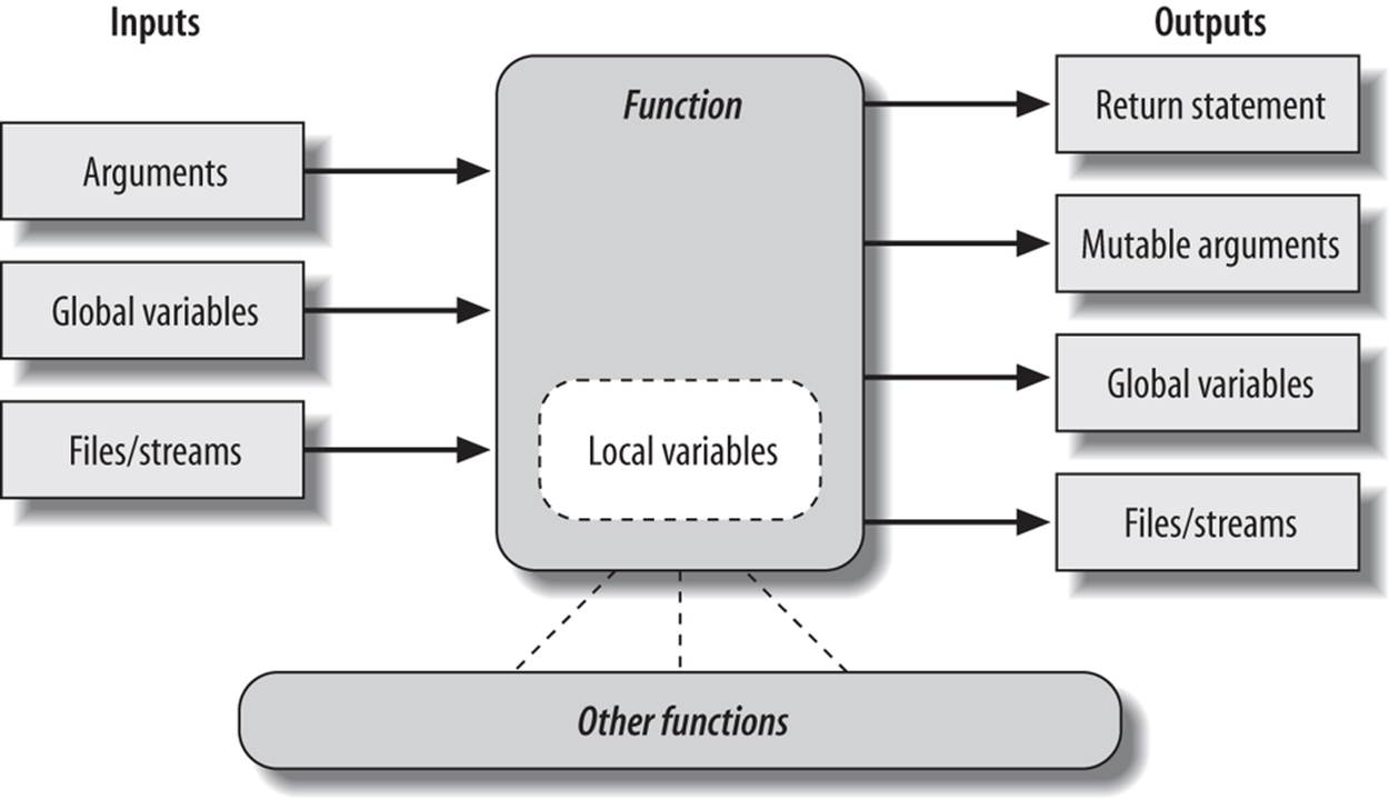
Figure 19-1. Function execution environment. Functions may obtain input and produce output in a variety of ways, though functions are usually easier to understand and maintain if you use arguments for input and return statements and anticipated mutable argument changes for output. In Python 3.X only, outputs may also take the form of declared nonlocal names that exist in an enclosing function scope.

Of course, there are plenty of exceptions to the preceding design rules, including some related to Python’s OOP support. As you’ll see in Part VI, Python classes depend on changing a passed-in mutable object—class functions set attributes of an automatically passed-in argument called selfto change per-object state information (e.g., self.name='bob'). Moreover, if classes are not used, global variables are often the most straightforward way for functions in modules to retain single-copy state between calls. Side effects are usually dangerous only if they’re unexpected.

In general though, you should strive to minimize external dependencies in functions and other program components. The more self-contained a function is, the easier it will be to understand, reuse, and modify.

Recursive Functions

We mentioned recursion in relation to comparisons of core types in Chapter 9. While discussing scope rules near the start of Chapter 17, we also briefly noted that Python supports recursive functions—functions that call themselves either directly or indirectly in order to loop. In this section, we’ll explore what this looks like in our functions’ code.

Recursion is a somewhat advanced topic, and it’s relatively rare to see in Python, partly because Python’s procedural statements include simpler looping structures. Still, it’s a useful technique to know about, as it allows programs to traverse structures that have arbitrary and unpredictable shapes and depths—planning travel routes, analyzing language, and crawling links on the Web, for example. Recursion is even an alternative to simple loops and iterations, though not necessarily the simplest or most efficient one.

Summation with Recursion

Let’s look at some examples. To sum a list (or other sequence) of numbers, we can either use the built-in sum function or write a more custom version of our own. Here’s what a custom summing function might look like when coded with recursion:

>>> def mysum(L):

if not L:

return 0

else:

return L[0] + mysum(L[1:]) # Call myself recursively

>>> mysum([1, 2, 3, 4, 5])

15

At each level, this function calls itself recursively to compute the sum of the rest of the list, which is later added to the item at the front. The recursive loop ends and zero is returned when the list becomes empty. When using recursion like this, each open level of call to the function has its own copy of the function’s local scope on the runtime call stack—here, that means L is different in each level.

If this is difficult to understand (and it often is for new programmers), try adding a print of L to the function and run it again, to trace the current list at each call level:

>>> def mysum(L):

print(L) # Trace recursive levels

if not L: # L shorter at each level

return 0

else:

return L[0] + mysum(L[1:])

>>> mysum([1, 2, 3, 4, 5])

[1, 2, 3, 4, 5]

[2, 3, 4, 5]

[3, 4, 5]

[4, 5]

[5]

[]

15

As you can see, the list to be summed grows smaller at each recursive level, until it becomes empty—the termination of the recursive loop. The sum is computed as the recursive calls unwind on returns.

Coding Alternatives

Interestingly, we can use Python’s if/else ternary expression (described in Chapter 12) to save some code real estate here. We can also generalize for any summable type (which is easier if we assume at least one item in the input, as we did in Chapter 18’s minimum value example) and use Python 3.X’s extended sequence assignment to make the first/rest unpacking simpler (as covered in Chapter 11):

def mysum(L):

return 0 if not L else L[0] + mysum(L[1:]) # Use ternary expression

def mysum(L):

return L[0] if len(L) == 1 else L[0] + mysum(L[1:]) # Any type, assume one

def mysum(L):

first, *rest = L

return first if not rest else first + mysum(rest) # Use 3.X ext seq assign

The latter two of these fail for empty lists but allow for sequences of any object type that supports +, not just numbers:

>>> mysum([1]) # mysum([]) fails in last 2

1

>>> mysum([1, 2, 3, 4, 5])

15

>>> mysum(('s', 'p', 'a', 'm')) # But various types now work

'spam'

>>> mysum(['spam', 'ham', 'eggs'])

'spamhameggs'

Run these on your own for more insight. If you study these three variants, you’ll find that:

§ The latter two also work on a single string argument (e.g., mysum('spam')), because strings are sequences of one-character strings.

§ The third variant works on arbitrary iterables, including open input files (mysum(open(name))), but the others do not because they index (Chapter 14 illustrates extended sequence assignment on files).

§ The function header def mysum(first, *rest), although similar to the third variant, wouldn’t work at all, because it expects individual arguments, not a single iterable.

Keep in mind that recursion can be direct, as in the examples so far, or indirect, as in the following (a function that calls another function, which calls back to its caller). The net effect is the same, though there are two function calls at each level instead of one:

>>> def mysum(L):

if not L: return 0

return nonempty(L) # Call a function that calls me

>>> def nonempty(L):

return L[0] + mysum(L[1:]) # Indirectly recursive

>>> mysum([1.1, 2.2, 3.3, 4.4])

11.0

Loop Statements Versus Recursion

Though recursion works for summing in the prior sections’ examples, it’s probably overkill in this context. In fact, recursion is not used nearly as often in Python as in more esoteric languages like Prolog or Lisp, because Python emphasizes simpler procedural statements like loops, which are usually more natural. The while, for example, often makes things a bit more concrete, and it doesn’t require that a function be defined to allow recursive calls:

>>> L = [1, 2, 3, 4, 5]

>>> sum = 0

>>> while L:

sum += L[0]

L = L[1:]

>>> sum

15

Better yet, for loops iterate for us automatically, making recursion largely extraneous in many cases (and, in all likelihood, less efficient in terms of memory space and execution time):

>>> L = [1, 2, 3, 4, 5]

>>> sum = 0

>>> for x in L: sum += x

>>> sum

15

With looping statements, we don’t require a fresh copy of a local scope on the call stack for each iteration, and we avoid the speed costs associated with function calls in general. (Stay tuned for Chapter 21’s timer case study for ways to compare the execution times of alternatives like these.)

Handling Arbitrary Structures

On the other hand, recursion—or equivalent explicit stack-based algorithms we’ll meet shortly—can be required to traverse arbitrarily shaped structures. As a simple example of recursion’s role in this context, consider the task of computing the sum of all the numbers in a nested sublists structure like this:

[1, [2, [3, 4], 5], 6, [7, 8]] # Arbitrarily nested sublists

Simple looping statements won’t work here because this is not a linear iteration. Nested looping statements do not suffice either, because the sublists may be nested to arbitrary depth and in an arbitrary shape—there’s no way to know how many nested loops to code to handle all cases. Instead, the following code accommodates such general nesting by using recursion to visit sublists along the way:

# file sumtree.py

def sumtree(L):

tot = 0

for x in L: # For each item at this level

if not isinstance(x, list):

tot += x # Add numbers directly

else:

tot += sumtree(x) # Recur for sublists

return tot

L = [1, [2, [3, 4], 5], 6, [7, 8]] # Arbitrary nesting

print(sumtree(L)) # Prints 36

# Pathological cases

print(sumtree([1, [2, [3, [4, [5]]]]])) # Prints 15 (right-heavy)

print(sumtree([[[[[1], 2], 3], 4], 5])) # Prints 15 (left-heavy)

Trace through the test cases at the bottom of this script to see how recursion traverses their nested lists.

Recursion versus queues and stacks

It sometimes helps to understand that internally, Python implements recursion by pushing information on a call stack at each recursive call, so it remembers where it must return and continue later. In fact, it’s generally possible to implement recursive-style procedures without recursive calls, by using an explicit stack or queue of your own to keep track of remaining steps.

For instance, the following computes the same sums as the prior example, but uses an explicit list to schedule when it will visit items in the subject, instead of issuing recursive calls; the item at the front of the list is always the next to be processed and summed:

def sumtree(L): # Breadth-first, explicit queue

tot = 0

items = list(L) # Start with copy of top level

while items:

front = items.pop(0) # Fetch/delete front item

if not isinstance(front, list):

tot += front # Add numbers directly

else:

items.extend(front) # <== Append all in nested list

return tot

Technically, this code traverses the list in breadth-first fashion by levels, because it adds nested lists’ contents to the end of the list, forming a first-in-first-out queue. To emulate the traversal of the recursive call version more closely, we can change it to perform depth-first traversal simply by adding the content of nested lists to the front of the list, forming a last-in-first-out stack:

def sumtree(L): # Depth-first, explicit stack

tot = 0

items = list(L) # Start with copy of top level

while items:

front = items.pop(0) # Fetch/delete front item

if not isinstance(front, list):

tot += front # Add numbers directly

else:

items[:0] = front # <== Prepend all in nested list

return tot

For more on the last two examples (and another variant), see file sumtree2.py in the book’s examples. It adds items list tracing so you can watch it grow in both schemes, and can show numbers as they are visited so you see the search order. For instance, the breadth-first and depth-first variants visit items in the same three test lists used for the recursive version in the following orders, respectively (sums are shown last):

c:\code> sumtree2.py

1, 6, 2, 5, 7, 8, 3, 4, 36

1, 2, 3, 4, 5, 15

5, 4, 3, 2, 1, 15

----------------------------------------

1, 2, 3, 4, 5, 6, 7, 8, 36

1, 2, 3, 4, 5, 15

1, 2, 3, 4, 5, 15

----------------------------------------

In general, though, once you get the hang of recursive calls, they are more natural than the explicit scheduling lists they automate, and are generally preferred unless you need to traverse structure in specialized ways. Some programs, for example, perform a best-first search that requires an explicit search queue ordered by relevance or other criteria. If you think of a web crawler that scores pages visited by content, the applications may start to become clearer.

Cycles, paths, and stack limits

As is, these programs suffice for our example, but larger recursive applications can sometimes require a bit more infrastructure than shown here: they may need to avoid cycles or repeats, record paths taken for later use, and expand stack space when using recursive calls instead of explicit queues or stacks.

For instance, neither the recursive call nor the explicit queue/stack examples in this section do anything about avoiding cycles—visiting a location already visited. That’s not required here, because we’re traversing strictly hierarchical list object trees. If data can be a cyclic graph, though, both these schemes will fail: the recursive call version will fall into an infinite recursive loop (and may run out of call-stack space), and the others will fall into simple infinite loops, re-adding the same items to their lists (and may or may not run out of general memory). Some programs also need to avoid repeated processing for a state reached more than once, even if that wouldn’t lead to a loop.

To do better, the recursive call version could simply keep and pass a set, dictionary, or list of states visited so far and check for repeats as it goes. We will use this scheme in later recursive examples in this book:

if state not in visited:

visited.add(state) # x.add(state), x[state]=True, or x.append(state)

...proceed...

The nonrecursive alternatives could similarly avoid adding states already visited with code like the following. Note that checking for duplicates already on the items list would avoid scheduling a state twice, but would not prevent revisiting a state traversed earlier and hence removed from that list:

visited.add(front)

...proceed...

items.extend([x for x in front if x not in visited])

This model doesn’t quite apply to this section’s use case that simply adds numbers in lists, but larger applications will be able to identify repeated states—a URL of a previously visited web page, for instance. In fact, we’ll use such techniques to avoid cycles and repeats in later examples listed in the next section.

Some programs may also need to record complete paths for each state followed so they can report solutions when finished. In such cases, each item in the nonrecursive scheme’s stack or queue may be a full path list that suffices for a record of states visited, and contains the next item to explore at either end.

Also note that standard Python limits the depth of its runtime call stack—crucial to recursive call programs—to trap infinite recursion errors. To expand it, use the sys module:

>>> sys.getrecursionlimit() # 1000 calls deep default

1000

>>> sys.setrecursionlimit(10000) # Allow deeper nesting

>>> help(sys.setrecursionlimit) # Read more about it

The maximum allowed setting can vary per platform. This isn’t required for programs that use stacks or queues to avoid recursive calls and gain more control over the traversal process.

More recursion examples

Although this section’s example is artificial, it is representative of a larger class of programs; inheritance trees and module import chains, for example, can exhibit similarly general structures, and computing structures such as permutations can require arbitrarily many nested loops. In fact, we will use recursion again in such roles in more realistic examples later in this book:

§ In Chapter 20’s permute.py, to shuffle arbitrary sequences

§ In Chapter 25’s reloadall.py, to traverse import chains

§ In Chapter 29’s classtree.py, to traverse class inheritance trees

§ In Chapter 31’s lister.py, to traverse class inheritance trees again

§ In Appendix D’s solutions to two exercises at the end of this part of the book: countdowns and factorials

The second and third of these will also detect states already visited to avoid cycles and repeats. Although simple loops should generally be preferred to recursion for linear iterations on the grounds of simplicity and efficiency, we’ll find that recursion is essential in scenarios like those in these later examples.

Moreover, you sometimes need to be aware of the potential of unintended recursion in your programs. As you’ll also see later in the book, some operator overloading methods in classes such as __setattr__ and __getattribute__ and even __repr__ have the potential to recursively loop if used incorrectly. Recursion is a powerful tool, but it tends to be best when both understood and expected!

Function Objects: Attributes and Annotations

Python functions are more flexible than you might think. As we’ve seen in this part of the book, functions in Python are much more than code-generation specifications for a compiler—Python functions are full-blown objects, stored in pieces of memory all their own. As such, they can be freely passed around a program and called indirectly. They also support operations that have little to do with calls at all—attribute storage and annotation.

Indirect Function Calls: “First Class” Objects

Because Python functions are objects, you can write programs that process them generically. Function objects may be assigned to other names, passed to other functions, embedded in data structures, returned from one function to another, and more, as if they were simple numbers or strings. Function objects also happen to support a special operation: they can be called by listing arguments in parentheses after a function expression. Still, functions belong to the same general category as other objects.

This is usually called a first-class object model; it’s ubiquitous in Python, and a necessary part of functional programming. We’ll explore this programming mode more fully in this and the next chapter; because its motif is founded on the notion of applying functions, functions must be treated as data.

We’ve seen some of these generic use cases for functions in earlier examples, but a quick review helps to underscore the object model. For example, there’s really nothing special about the name used in a def statement: it’s just a variable assigned in the current scope, as if it had appeared on the left of an = sign. After a def runs, the function name is simply a reference to an object—you can reassign that object to other names freely and call it through any reference:

>>> def echo(message): # Name echo assigned to function object

print(message)

>>> echo('Direct call') # Call object through original name

Direct call

>>> x = echo # Now x references the function too

>>> x('Indirect call!') # Call object through name by adding ()

Indirect call!

Because arguments are passed by assigning objects, it’s just as easy to pass functions to other functions as arguments. The callee may then call the passed-in function just by adding arguments in parentheses:

>>> def indirect(func, arg):

func(arg) # Call the passed-in object by adding ()

>>> indirect(echo, 'Argument call!') # Pass the function to another function

Argument call!

You can even stuff function objects into data structures, as though they were integers or strings. The following, for example, embeds the function twice in a list of tuples, as a sort of actions table. Because Python compound types like these can contain any sort of object, there’s no special case here, either:

>>> schedule = [ (echo, 'Spam!'), (echo, 'Ham!') ]

>>> for (func, arg) in schedule:

func(arg) # Call functions embedded in containers

Spam!

Ham!

This code simply steps through the schedule list, calling the echo function with one argument each time through (notice the tuple-unpacking assignment in the for loop header, introduced in Chapter 13). As we saw in Chapter 17’s examples, functions can also be created and returned for use elsewhere—the closure created in this mode also retains state from the enclosing scope:

>>> def make(label): # Make a function but don't call it

def echo(message):

print(label + ':' + message)

return echo

>>> F = make('Spam') # Label in enclosing scope is retained

>>> F('Ham!') # Call the function that make returned

Spam:Ham!

>>> F('Eggs!')

Spam:Eggs!

Python’s universal first-class object model and lack of type declarations make for an incredibly flexible programming language.

Function Introspection

Because they are objects, we can also process functions with normal object tools. In fact, functions are more flexible than you might expect. For instance, once we make a function, we can call it as usual:

>>> def func(a):

b = 'spam'

return b * a

>>> func(8)

'spamspamspamspamspamspamspamspam'

But the call expression is just one operation defined to work on function objects. We can also inspect their attributes generically (the following is run in Python 3.3, but 2.X results are similar):

>>> func.__name__

'func'

>>> dir(func)

['__annotations__', '__call__', '__class__', '__closure__', '__code__',

...more omitted: 34 total...

'__repr__', '__setattr__', '__sizeof__', '__str__', '__subclasshook__']

Introspection tools allow us to explore implementation details too—functions have attached code objects, for example, which provide details on aspects such as the functions’ local variables and arguments:

>>> func.__code__

<code object func at 0x00000000021A6030, file "<stdin>", line 1>

>>> dir(func.__code__)

['__class__', '__delattr__', '__dir__', '__doc__', '__eq__', '__format__', '__ge__',

...more omitted: 37 total...

'co_argcount', 'co_cellvars', 'co_code', 'co_consts', 'co_filename',

'co_firstlineno', 'co_flags', 'co_freevars', 'co_kwonlyargcount', 'co_lnotab',

'co_name', 'co_names', 'co_nlocals', 'co_stacksize', 'co_varnames']

>>> func.__code__.co_varnames

('a', 'b')

>>> func.__code__.co_argcount

1

Tool writers can make use of such information to manage functions (in fact, we will too in Chapter 39, to implement validation of function arguments in decorators).

Function Attributes

Function objects are not limited to the system-defined attributes listed in the prior section, though. As we learned in Chapter 17, it’s been possible to attach arbitrary user-defined attributes to them as well since Python 2.1:

>>> func

<function func at 0x000000000296A1E0>

>>> func.count = 0

>>> func.count += 1

>>> func.count

1

>>> func.handles = 'Button-Press'

>>> func.handles

'Button-Press'

>>> dir(func)

['__annotations__', '__call__', '__class__', '__closure__', '__code__',

...and more: in 3.X all others have double underscores so your names won't clash...

__str__', '__subclasshook__', 'count', 'handles']

Python’s own implementation-related data stored on functions follows naming conventions that prevent them from clashing with the more arbitrary attribute names you might assign yourself. In 3.X, all function internals’ names have leading and trailing double underscores (“__X__”); 2.X follows the same scheme, but also assigns some names that begin with “func_X”:

c:\code> py −3

>>> def f(): pass

>>> dir(f)

...run on your own to see...

>>> len(dir(f))

34

>>> [x for x in dir(f) if not x.startswith('__')]

[]

c:\code> py −2

>>> def f(): pass

>>> dir(f)

...run on your own to see...

>>> len(dir(f))

31

>>> [x for x in dir(f) if not x.startswith('__')]

['func_closure', 'func_code', 'func_defaults', 'func_dict', 'func_doc',

'func_globals', 'func_name']

If you’re careful not to name attributes the same way, you can safely use the function’s namespace as though it were your own namespace or scope.

As we saw in that chapter, such attributes can be used to attach state information to function objects directly, instead of using other techniques such as globals, nonlocals, and classes. Unlike nonlocals, such attributes are accessible anywhere the function itself is, even from outside its code.

In a sense, this is also a way to emulate “static locals” in other languages—variables whose names are local to a function, but whose values are retained after a function exits. Attributes are related to objects instead of scopes (and must be referenced through the function name within its code), but the net effect is similar.

Moreover, as we learned in Chapter 17, when attributes are attached to functions generated by other factory functions, they also support multiple copy, per-call, and writeable state retention, much like nonlocal closures and class instance attributes.

Function Annotations in 3.X

In Python 3.X (but not 2.X), it’s also possible to attach annotation information—arbitrary user-defined data about a function’s arguments and result—to a function object. Python provides special syntax for specifying annotations, but it doesn’t do anything with them itself; annotations are completely optional, and when present are simply attached to the function object’s __annotations__ attribute for use by other tools. For instance, such a tool might use annotations in the context of error testing.

We met Python 3.X’s keyword-only arguments in the preceding chapter; annotations generalize function header syntax further. Consider the following nonannotated function, which is coded with three arguments and returns a result:

>>> def func(a, b, c):

return a + b + c

>>> func(1, 2, 3)

6

Syntactically, function annotations are coded in def header lines, as arbitrary expressions associated with arguments and return values. For arguments, they appear after a colon immediately following the argument’s name; for return values, they are written after a -> following the arguments list. This code, for example, annotates all three of the prior function’s arguments, as well as its return value:

>>> def func(a: 'spam', b: (1, 10), c: float) -> int:

return a + b + c

>>> func(1, 2, 3)

6

Calls to an annotated function work as usual, but when annotations are present Python collects them in a dictionary and attaches it to the function object itself. Argument names become keys, the return value annotation is stored under key “return” if coded (which suffices because this reserved word can’t be used as an argument name), and the values of annotation keys are assigned to the results of the annotation expressions:

>>> func.__annotations__

{'c': <class 'float'>, 'b': (1, 10), 'a': 'spam', 'return': <class 'int'>}

Because they are just Python objects attached to a Python object, annotations are straightforward to process. The following annotates just two of three arguments and steps through the attached annotations generically:

>>> def func(a: 'spam', b, c: 99):

return a + b + c

>>> func(1, 2, 3)

6

>>> func.__annotations__

{'c': 99, 'a': 'spam'}

>>> for arg in func.__annotations__:

print(arg, '=>', func.__annotations__[arg])

c => 99

a => spam

There are two fine points to note here. First, you can still use defaults for arguments if you code annotations—the annotation (and its : character) appear before the default (and its = character). In the following, for example, a: 'spam' = 4 means that argument a defaults to 4 and is annotated with the string 'spam':

>>> def func(a: 'spam' = 4, b: (1, 10) = 5, c: float = 6) -> int:

return a + b + c

>>> func(1, 2, 3)

6

>>> func() # 4 + 5 + 6 (all defaults)

15

>>> func(1, c=10) # 1 + 5 + 10 (keywords work normally)

16

>>> func.__annotations__

{'c': <class 'float'>, 'b': (1, 10), 'a': 'spam', 'return': <class 'int'>}

Second, note that the blank spaces in the prior example are all optional—you can use spaces between components in function headers or not, but omitting them might degrade your code’s readability to some observers (and probably improve it to others!):

>>> def func(a:'spam'=4, b:(1,10)=5, c:float=6)->int:

return a + b + c

>>> func(1, 2) # 1 + 2 + 6

9

>>> func.__annotations__

{'c': <class 'float'>, 'b': (1, 10), 'a': 'spam', 'return': <class 'int'>}

Annotations are a new feature in 3.X, and some of their potential uses remain to be uncovered. It’s easy to imagine annotations being used to specify constraints for argument types or values, though, and larger APIs might use this feature as a way to register function interface information.

In fact, we’ll see a potential application in Chapter 39, where we’ll look at annotations as an alternative to function decorator arguments—a more general concept in which information is coded outside the function header and so is not limited to a single role. Like Python itself, annotation is a tool whose roles are shaped by your imagination.

Finally, note that annotations work only in def statements, not lambda expressions, because lambda’s syntax already limits the utility of the functions it defines. Coincidentally, this brings us to our next topic.

Anonymous Functions: lambda

Besides the def statement, Python also provides an expression form that generates function objects. Because of its similarity to a tool in the Lisp language, it’s called lambda.^[39^] Like def, this expression creates a function to be called later, but it returns the function instead of assigning it to a name. This is why lambdas are sometimes known as anonymous (i.e., unnamed) functions. In practice, they are often used as a way to inline a function definition, or to defer execution of a piece of code.

lambda Basics

The lambda’s general form is the keyword lambda, followed by one or more arguments (exactly like the arguments list you enclose in parentheses in a def header), followed by an expression after a colon:

lambda argument1, argument2,... argumentN : expression using arguments

Function objects returned by running lambda expressions work exactly the same as those created and assigned by defs, but there are a few differences that make lambdas useful in specialized roles:

§ lambda is an expression, not a statement. Because of this, a lambda can appear in places a def is not allowed by Python’s syntax—inside a list literal or a function call’s arguments, for example. With def, functions can be referenced by name but must be created elsewhere. As an expression, lambda returns a value (a new function) that can optionally be assigned a name. In contrast, the def statement always assigns the new function to the name in the header, instead of returning it as a result.

§ lambda’s body is a single expression, not a block of statements. The lambda’s body is similar to what you’d put in a def body’s return statement; you simply type the result as a naked expression, instead of explicitly returning it. Because it is limited to an expression, a lambda is less general than a def—you can only squeeze so much logic into a lambda body without using statements such as if. This is by design, to limit program nesting: lambda is designed for coding simple functions, and def handles larger tasks.

Apart from those distinctions, defs and lambdas do the same sort of work. For instance, we’ve seen how to make a function with a def statement:

>>> def func(x, y, z): return x + y + z

>>> func(2, 3, 4)

9

But you can achieve the same effect with a lambda expression by explicitly assigning its result to a name through which you can later call the function:

>>> f = lambda x, y, z: x + y + z

>>> f(2, 3, 4)

9

Here, f is assigned the function object the lambda expression creates; this is how def works, too, but its assignment is automatic.

Defaults work on lambda arguments, just like in a def:

>>> x = (lambda a="fee", b="fie", c="foe": a + b + c)

>>> x("wee")

'weefiefoe'

The code in a lambda body also follows the same scope lookup rules as code inside a def. lambda expressions introduce a local scope much like a nested def, which automatically sees names in enclosing functions, the module, and the built-in scope (via the LEGB rule, and perChapter 17):

>>> def knights():

title = 'Sir'

action = (lambda x: title + ' ' + x) # Title in enclosing def scope

return action # Return a function object

>>> act = knights()

>>> msg = act('robin') # 'robin' passed to x

>>> msg

'Sir robin'

>>> act # act: a function, not its result

<function knights.<locals>.<lambda> at 0x00000000029CA488>

In this example, prior to Release 2.2, the value for the name title would typically have been passed in as a default argument value instead; flip back to the scopes coverage in Chapter 17 if you’ve forgotten why.

Why Use lambda?

Generally speaking, lambda comes in handy as a sort of function shorthand that allows you to embed a function’s definition within the code that uses it. They are entirely optional—you can always use def instead, and should if your function requires the power of full statements that thelambda’s expression cannot easily provide—but they tend to be simpler coding constructs in scenarios where you just need to embed small bits of executable code inline at the place it is to be used.

For instance, we’ll see later that callback handlers are frequently coded as inline lambda expressions embedded directly in a registration call’s arguments list, instead of being defined with a def elsewhere in a file and referenced by name (see the sidebar Why You Will Care: lambda Callbacks for an example).

lambda is also commonly used to code jump tables, which are lists or dictionaries of actions to be performed on demand. For example:

L = [lambda x: x ** 2, # Inline function definition

lambda x: x ** 3,

lambda x: x ** 4] # A list of three callable functions

for f in L:

print(f(2)) # Prints 4, 8, 16

print(L[0](3)) # Prints 9

The lambda expression is most useful as a shorthand for def, when you need to stuff small pieces of executable code into places where statements are illegal syntactically. The preceding code snippet, for example, builds up a list of three functions by embedding lambda expressions inside a list literal; a def won’t work inside a list literal like this because it is a statement, not an expression. The equivalent def coding would require temporary function names (which might clash with others) and function definitions outside the context of intended use (which might be hundreds of lines away):

def f1(x): return x ** 2

def f2(x): return x ** 3 # Define named functions

def f3(x): return x ** 4

L = [f1, f2, f3] # Reference by name

for f in L:

print(f(2)) # Prints 4, 8, 16

print(L[0](3)) # Prints 9

Multiway branch switches: The finale

In fact, you can do the same sort of thing with dictionaries and other data structures in Python to build up more general sorts of action tables. Here’s another example to illustrate, at the interactive prompt:

>>> key = 'got'

>>> {'already': (lambda: 2 + 2),

'got': (lambda: 2 * 4),

'one': (lambda: 2 ** 6)}[key]()

8

Here, when Python makes the temporary dictionary, each of the nested lambdas generates and leaves behind a function to be called later. Indexing by key fetches one of those functions, and parentheses force the fetched function to be called. When coded this way, a dictionary becomes a more general multiway branching tool than what I could fully show you in Chapter 12’s coverage of if statements.

To make this work without lambda, you’d need to instead code three def statements somewhere else in your file, outside the dictionary in which the functions are to be used, and reference the functions by name:

>>> def f1(): return 2 + 2

>>> def f2(): return 2 * 4

>>> def f3(): return 2 ** 6

>>> key = 'one'

>>> {'already': f1, 'got': f2, 'one': f3}[key]()

64

This works, too, but your defs may be arbitrarily far away in your file, even if they are just little bits of code. The code proximity that lambdas provide is especially useful for functions that will only be used in a single context—if the three functions here are not useful anywhere else, it makes sense to embed their definitions within the dictionary as lambdas. Moreover, the def form requires you to make up names for these little functions that may clash with other names in this file (perhaps unlikely, but always possible).^[40^]

lambdas also come in handy in function-call argument lists as a way to inline temporary function definitions not used anywhere else in your program; we’ll see some examples of such other uses later in this chapter, when we study map.

How (Not) to Obfuscate Your Python Code

The fact that the body of a lambda has to be a single expression (not a series of statements) would seem to place severe limits on how much logic you can pack into a lambda. If you know what you’re doing, though, you can code most statements in Python as expression-based equivalents.

For example, if you want to print from the body of a lambda function, simply say print(X) in Python 3.X where this becomes a call expression instead of a statement, or say sys.stdout.write(str(X)+'\n') in either Python 2.X or 3.X to make sure it’s an expression portably (recall from Chapter 11 that this is what print really does). Similarly, to nest selection logic in a lambda, you can use the if/else ternary expression introduced in Chapter 12, or the equivalent but trickier and/or combination also described there. As you learned earlier, the following statement:

if a:

b

else:

c

can be emulated by either of these roughly equivalent expressions:

b if a else c

((a and b) or c)

Because expressions like these can be placed inside a lambda, they may be used to implement selection logic within a lambda function:

>>> lower = (lambda x, y: x if x < y else y)

>>> lower('bb', 'aa')

'aa'

>>> lower('aa', 'bb')

'aa'

Furthermore, if you need to perform loops within a lambda, you can also embed things like map calls and list comprehension expressions—tools we met in earlier chapters and will revisit in this and the next chapter:

>>> import sys

>>> showall = lambda x: list(map(sys.stdout.write, x)) # 3.X: must use list

>>> t = showall(['spam\n', 'toast\n', 'eggs\n']) # 3.X: can use print

spam

toast

eggs

>>> showall = lambda x: [sys.stdout.write(line) for line in x]

>>> t = showall(('bright\n', 'side\n', 'of\n', 'life\n'))

bright

side

of

life

>>> showall = lambda x: [print(line, end='') for line in x] # Same: 3.X only

>>> showall = lambda x: print(*x, sep='', end='') # Same: 3.X only

There is a limit to emulating statements with expressions: you can’t directly achieve an assignment statement’s effect, for instance, though tools like the setattr built-in, the __dict__ of namespaces, and methods that change mutable objects in place can sometimes stand in, and functional programming techniques can take you deep into the dark realm of convoluted expression.

Now that I’ve shown you these tricks, I am required to ask you to please only use them as a last resort. Without due care, they can lead to unreadable (a.k.a. obfuscated) Python code. In general, simple is better than complex, explicit is better than implicit, and full statements are better than arcane expressions. That’s why lambda is limited to expressions. If you have larger logic to code, use def; lambda is for small pieces of inline code. On the other hand, you may find these techniques useful in moderation.

Scopes: lambdas Can Be Nested Too

lambdas are the main beneficiaries of nested function scope lookup (the E in the LEGB scope rule we studied in Chapter 17). As a review, in the following the lambda appears inside a def—the typical case—and so can access the value that the name x had in the enclosing function’s scope at the time that the enclosing function was called:

>>> def action(x):

return (lambda y: x + y) # Make and return function, remember x

>>> act = action(99)

>>> act

<function action.<locals>.<lambda> at 0x00000000029CA2F0>

>>> act(2) # Call what action returned

101

What wasn’t illustrated in the prior discussion of nested function scopes is that a lambda also has access to the names in any enclosing lambda. This case is somewhat obscure, but imagine if we recoded the prior def with a lambda:

>>> action = (lambda x: (lambda y: x + y))

>>> act = action(99)

>>> act(3)

102

>>> ((lambda x: (lambda y: x + y))(99))(4)

103

Here, the nested lambda structure makes a function that makes a function when called. In both cases, the nested lambda’s code has access to the variable x in the enclosing lambda. This works, but it seems fairly convoluted code; in the interest of readability, nested lambdas are generallybest avoided.

WHY YOU WILL CARE: LAMBDA CALLBACKS

Another very common application of lambda is to define inline callback functions for Python’s tkinter GUI API (this module is named Tkinter in Python 2.X). For example, the following creates a button that prints a message on the console when pressed, assuming tkinter is available on your computer (it is by default on Windows, Mac, Linux, and other OSs):

import sys

from tkinter import Button, mainloop # Tkinter in 2.X

x = Button(

text='Press me',

command=(lambda:sys.stdout.write('Spam\n'))) # 3.X: print()

x.pack()

mainloop() # This may be optional in console mode

Here, we register the callback handler by passing a function generated with a lambda to the command keyword argument. The advantage of lambda over def here is that the code that handles a button press is right here, embedded in the button-creation call.

In effect, the lambda defers execution of the handler until the event occurs: the write call happens on button presses, not when the button is created, and effectively “knows” the string it should write when the event occurs.

Because the nested function scope rules apply to lambdas as well, they are also easier to use as callback handlers, as of Python 2.2—they automatically see names in the functions in which they are coded and no longer require passed-in defaults in most cases. This is especially handy for accessing the special self instance argument that is a local variable in enclosing class method functions (more on classes in Part VI):

class MyGui:

def makewidgets(self):

Button(command=(lambda: self.onPress("spam")))

def onPress(self, message):

...use message...

In early versions of Python, even self had to be passed in to a lambda with defaults. As we’ll see later, class objects with __call__ and bound methods often serve in callback roles too—watch for coverage of these in Chapter 30 and Chapter 31.