Neural Networks - Data Science from Scratch: First Principles with Python (2015)

Data Science from Scratch: First Principles with Python (2015)

Chapter 18. Neural Networks

I like nonsense; it wakes up the brain cells.

Dr. Seuss

An artificial neural network (or neural network for short) is a predictive model motivated by the way the brain operates. Think of the brain as a collection of neurons wired together. Each neuron looks at the outputs of the other neurons that feed into it, does a calculation, and then either fires (if the calculation exceeds some threshhold) or doesn’t (if it doesn’t).

Accordingly, artificial neural networks consist of artificial neurons, which perform similar calculations over their inputs. Neural networks can solve a wide variety of problems like handwriting recognition and face detection, and they are used heavily in deep learning, one of the trendiest subfields of data science. However, most neural networks are “black boxes” — inspecting their details doesn’t give you much understanding of how they’re solving a problem. And large neural networks can be difficult to train. For most problems you’ll encounter as a budding data scientist, they’re probably not the right choice. Someday, when you’re trying to build an artificial intelligence to bring about the Singularity, they very well might be.

Perceptrons

Pretty much the simplest neural network is the perceptron, which approximates a single neuron with n binary inputs. It computes a weighted sum of its inputs and “fires” if that weighted sum is zero or greater:

def step_function(x):
    return 1 if x >= 0 else 0
 
def perceptron_output(weights, bias, x):
    """returns 1 if the perceptron 'fires', 0 if not"""
    calculation = dot(weights, x) + bias
    return step_function(calculation)

The perceptron is simply distinguishing between the half spaces separated by the hyperplane of points x for which:

dot(weights,x) + bias == 0

With properly chosen weights, perceptrons can solve a number of simple problems (Figure 18-1). For example, we can create an AND gate (which returns 1 if both its inputs are 1 but returns 0 if one of its inputs is 0) with:

weights = [2, 2]
bias = -3

If both inputs are 1, the calculation equals 2 + 2 - 3 = 1, and the output is 1. If only one of the inputs is 1, the calculation equals 2 + 0 - 3 = -1, and the output is 0. And if both of the inputs are 0, the calculation equals -3, and the output is 0.

Similarly, we could build an OR gate with:

weights = [2, 2]
bias = -1

Perceptron.

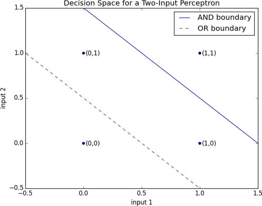
Figure 18-1. Decision space for a two-input perceptron

And we could build a NOT gate (which has one input and converts 1 to 0 and 0 to 1) with:

weights = [-2]
bias = 1

However, there are some problems that simply can’t be solved by a single perceptron. For example, no matter how hard you try, you cannot use a perceptron to build an XOR gate that outputs 1 if exactly one of its inputs is 1 and 0 otherwise. This is where we start needing more-complicated neural networks.

Of course, you don’t need to approximate a neuron in order to build a logic gate:

and_gate = min
or_gate = max
xor_gate = lambda x, y: 0 if x == y else 1

Like real neurons, artificial neurons start getting more interesting when you start connecting them together.

Feed-Forward Neural Networks

The topology of the brain is enormously complicated, so it’s common to approximate it with an idealized feed-forward neural network that consists of discrete layers of neurons, each connected to the next. This typically entails an input layer (which receives inputs and feeds them forward unchanged), one or more “hidden layers” (each of which consists of neurons that take the outputs of the previous layer, performs some calculation, and passes the result to the next layer), and an output layer (which produces the final outputs).

Just like the perceptron, each (noninput) neuron has a weight corresponding to each of its inputs and a bias. To make our representation simpler, we’ll add the bias to the end of our weights vector and give each neuron a bias input that always equals 1.

As with the perceptron, for each neuron we’ll sum up the products of its inputs and its weights. But here, rather than outputting the step_function applied to that product, we’ll output a smooth approximation of the step function. In particular, we’ll use the sigmoid function (Figure 18-2):

def sigmoid(t):
    return 1 / (1 + math.exp(-t))

Sigmoid.

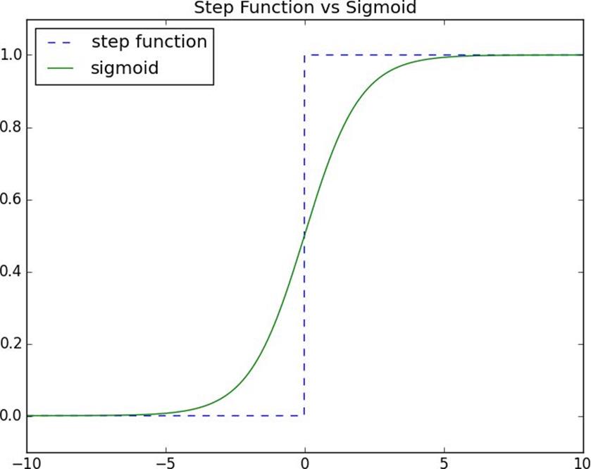
Figure 18-2. The sigmoid function

Why use sigmoid instead of the simpler step_function? In order to train a neural network, we’ll need to use calculus, and in order to use calculus, we need smooth functions. The step function isn’t even continuous, and sigmoid is a good smooth approximation of it.

NOTE

You may remember sigmoid from Chapter 16, where it was called logistic. Technically “sigmoid” refers to the shape of the function, “logistic” to this particular function although people often use the terms interchangeably.

We then calculate the output as:

def neuron_output(weights, inputs):
    return sigmoid(dot(weights, inputs))

Given this function, we can represent a neuron simply as a list of weights whose length is one more than the number of inputs to that neuron (because of the bias weight). Then we can represent a neural network as a list of (noninput) layers, where each layer is just a list of the neurons in that layer.

That is, we’ll represent a neural network as a list (layers) of lists (neurons) of lists (weights).

Given such a representation, using the neural network is quite simple:

def feed_forward(neural_network, input_vector):
    """takes in a neural network
    (represented as a list of lists of lists of weights)
    and returns the output from forward-propagating the input"""
 
    outputs = []
 
    # process one layer at a time
    for layer in neural_network:
        input_with_bias = input_vector + [1]              # add a bias input
        output = [neuron_output(neuron, input_with_bias)  # compute the output
                  for neuron in layer]                    # for each neuron
        outputs.append(output)                            # and remember it
 
        # then the input to the next layer is the output of this one
        input_vector = output
 
    return outputs

Now it’s easy to build the XOR gate that we couldn’t build with a single perceptron. We just need to scale the weights up so that the neuron_outputs are either really close to 0 or really close to 1:

xor_network = [# hidden layer
               [[20, 20, -30],      # 'and' neuron
                [20, 20, -10]],     # 'or'  neuron
               # output layer
               [[-60, 60, -30]]]    # '2nd input but not 1st input' neuron
 
for x in [0, 1]:
    for y in [0, 1]:
        # feed_forward produces the outputs of every neuron
        # feed_forward[-1] is the outputs of the output-layer neurons
        print x, y, feed_forward(xor_network,[x, y])[-1]
 
# 0 0 [9.38314668300676e-14]
# 0 1 [0.9999999999999059]
# 1 0 [0.9999999999999059]
# 1 1 [9.383146683006828e-14]

By using a hidden layer, we are able to feed the output of an “and” neuron and the output of an “or” neuron into a “second input but not first input” neuron. The result is a network that performs “or, but not and,” which is precisely XOR (Figure 18-3).

Neural Network.

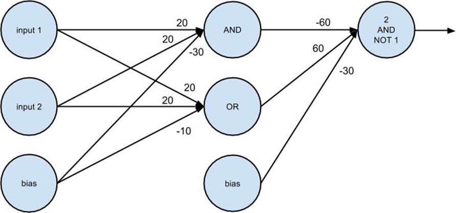
Figure 18-3. A neural network for XOR

Backpropagation

Usually we don’t build neural networks by hand. This is in part because we use them to solve much bigger problems — an image recognition problem might involve hundreds or thousands of neurons. And it’s in part because we usually won’t be able to “reason out” what the neurons should be.

Instead (as usual) we use data to train neural networks. One popular approach is an algorithm called backpropagation that has similarities to the gradient descent algorithm we looked at earlier.

Imagine we have a training set that consists of input vectors and corresponding target output vectors. For example, in our previous xor_network example, the input vector [1, 0] corresponded to the target output [1]. And imagine that our network has some set of weights. We then adjust the weights using the following algorithm:

1. Run feed_forward on an input vector to produce the outputs of all the neurons in the network.

2. This results in an error for each output neuron — the difference between its output and its target.

3. Compute the gradient of this error as a function of the neuron’s weights, and adjust its weights in the direction that most decreases the error.

4. “Propagate” these output errors backward to infer errors for the hidden layer.

5. Compute the gradients of these errors and adjust the hidden layer’s weights in the same manner.

Typically we run this algorithm many times for our entire training set until the network converges:

def backpropagate(network, input_vector, targets):
 
    hidden_outputs, outputs = feed_forward(network, input_vector)
 
    # the output * (1 - output) is from the derivative of sigmoid
    output_deltas = [output * (1 - output) * (output - target)
                     for output, target in zip(outputs, targets)]
 
    # adjust weights for output layer, one neuron at a time
    for i, output_neuron in enumerate(network[-1]):
        # focus on the ith output layer neuron
        for j, hidden_output in enumerate(hidden_outputs + [1]):
            # adjust the jth weight based on both
            # this neuron's delta and its jth input
            output_neuron[j] -= output_deltas[i] * hidden_output
 
    # back-propagate errors to hidden layer
    hidden_deltas = [hidden_output * (1 - hidden_output) *
                      dot(output_deltas, [n[i] for n in output_layer])
                     for i, hidden_output in enumerate(hidden_outputs)]
 
    # adjust weights for hidden layer, one neuron at a time
    for i, hidden_neuron in enumerate(network[0]):
        for j, input in enumerate(input_vector + [1]):
            hidden_neuron[j] -= hidden_deltas[i] * input

This is pretty much doing the same thing as if you explicitly wrote the squared error as a function of the weights and used the minimize_stochastic function we built in Chapter 8.

In this case, explicitly writing out the gradient function turns out to be kind of a pain. If you know calculus and the chain rule, the mathematical details are relatively straightforward, but keeping the notation straight (“the partial derivative of the error function with respect to the weight that neuron i assigns to the input coming from neuron j”) is not much fun.

Example: Defeating a CAPTCHA

To make sure that people registering for your site are actually people, the VP of Product Management wants to implement a CAPTCHA as part of the registration process. In particular, he’d like to show users a picture of a digit and require them to input that digit to prove they’re human.

He doesn’t believe you that computers can easily solve this problem, so you decide to convince him by creating a program that can easily solve the problem.

We’ll represent each digit as a 5 × 5 image:

@@@@@  ..@..  @@@@@  @@@@@  @...@  @@@@@  @@@@@  @@@@@  @@@@@  @@@@@
@...@  ..@..  ....@  ....@  @...@  @....  @....  ....@  @...@  @...@
@...@  ..@..  @@@@@  @@@@@  @@@@@  @@@@@  @@@@@  ....@  @@@@@  @@@@@
@...@  ..@..  @....  ....@  ....@  ....@  @...@  ....@  @...@  ....@
@@@@@  ..@..  @@@@@  @@@@@  ....@  @@@@@  @@@@@  ....@  @@@@@  @@@@@

Our neural network wants an input to be a vector of numbers. So we’ll transform each image to a vector of length 25, whose elements are either 1 (“this pixel is in the image”) or 0 (“this pixel is not in the image”).

For instance, the zero digit would be represented as:

zero_digit = [1,1,1,1,1,
              1,0,0,0,1,
              1,0,0,0,1,
              1,0,0,0,1,
              1,1,1,1,1]

We’ll want our output to indicate which digit the neural network thinks it is, so we’ll need 10 outputs. The correct output for digit 4, for instance, will be:

[0, 0, 0, 0, 1, 0, 0, 0, 0, 0]

Then, assuming our inputs are correctly ordered from 0 to 9, our targets will be:

targets = [[1 if i == j else 0 for i in range(10)]
           for j in range(10)]

so that (for example) targets[4] is the correct output for digit 4.

At which point we’re ready to build our neural network:

random.seed(0)      # to get repeatable results
input_size = 25     # each input is a vector of length 25
num_hidden = 5      # we'll have 5 neurons in the hidden layer
output_size = 10    # we need 10 outputs for each input
 
# each hidden neuron has one weight per input, plus a bias weight
hidden_layer = [[random.random() for __ in range(input_size + 1)]
                for __ in range(num_hidden)]
 
# each output neuron has one weight per hidden neuron, plus a bias weight
output_layer = [[random.random() for __ in range(num_hidden + 1)]
                for __ in range(output_size)]
 
# the network starts out with random weights
network = [hidden_layer, output_layer]

And we can train it using the backpropagation algorithm:

# 10,000 iterations seems enough to converge
for __ in range(10000):
    for input_vector, target_vector in zip(inputs, targets):
        backpropagate(network, input_vector, target_vector)

It works well on the training set, obviously:

def predict(input):
    return feed_forward(network, input)[-1]
 
predict(inputs[7])
# [0.026, 0.0, 0.0, 0.018, 0.001, 0.0, 0.0, 0.967, 0.0, 0.0]

Which indicates that the digit 7 output neuron produces 0.97, while all the other output neurons produce very small numbers.

But we can also apply it to differently drawn digits, like my stylized 3:

predict([0,1,1,1,0,  # .@@@.
         0,0,0,1,1,  # ...@@
         0,0,1,1,0,  # ..@@.
         0,0,0,1,1,  # ...@@
         0,1,1,1,0]) # .@@@.
 
# [0.0, 0.0, 0.0, 0.92, 0.0, 0.0, 0.0, 0.01, 0.0, 0.12]

The network still thinks it looks like a 3, whereas my stylized 8 gets votes for being a 5, an 8, and a 9:

predict([0,1,1,1,0,  # .@@@.
         1,0,0,1,1,  # @..@@
         0,1,1,1,0,  # .@@@.
         1,0,0,1,1,  # @..@@
         0,1,1,1,0]) # .@@@.
 
# [0.0, 0.0, 0.0, 0.0, 0.0, 0.55, 0.0, 0.0, 0.93, 1.0]

Having a larger training set would probably help.

Although the network’s operation is not exactly transparent, we can inspect the weights of the hidden layer to get a sense of what they’re recognizing. In particular, we can plot the weights of each neuron as a 5 × 5 grid corresponding to the 5 × 5 inputs.

In real life you’d probably want to plot zero weights as white, with larger positive weights more and more (say) green and larger negative weights more and more (say) red. Unfortunately, that’s hard to do in a black-and-white book.

Instead, we’ll plot zero weights as white, with far-away-from-zero weights darker and darker. And we’ll use crosshatching to indicate negative weights.

To do this we’ll use pyplot.imshow, which we haven’t seen before. With it we can plot images pixel by pixel. Normally this isn’t all that useful for data science, but here it’s a good choice:

import matplotlib
weights = network[0][0]               # first neuron in hidden layer
abs_weights = map(abs, weights)       # darkness only depends on absolute value
 
 
grid = [abs_weights[row:(row+5)]      # turn the weights into a 5x5 grid
        for row in range(0,25,5)]     # [weights[0:5], ..., weights[20:25]]
 
ax = plt.gca()                        # to use hatching, we'll need the axis
 
ax.imshow(grid,                       # here same as plt.imshow
          cmap=matplotlib.cm.binary,  # use white-black color scale
          interpolation='none')       # plot blocks as blocks
 
def patch(x, y, hatch, color):
    """return a matplotlib 'patch' object with the specified
    location, crosshatch pattern, and color"""
    return matplotlib.patches.Rectangle((x - 0.5, y - 0.5), 1, 1,
                                        hatch=hatch, fill=False, color=color)
 
# cross-hatch the negative weights
for i in range(5):                    # row
    for j in range(5):                # column
        if weights[5*i + j] < 0:      # row i, column j = weights[5*i + j]
            # add black and white hatches, so visible whether dark or light
            ax.add_patch(patch(j, i, '/',  "white"))
            ax.add_patch(patch(j, i, '\\', "black"))
 
plt.show()

Hidden Layer.

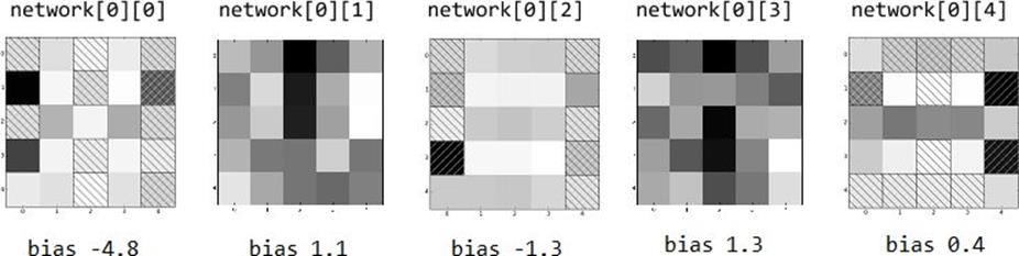
Figure 18-4. Weights for the hidden layer

In Figure 18-4 we see that the first hidden neuron has large positive weights in the left column and in the center of the middle row, while it has large negative weights in the right column. (And you can see that it has a pretty large negative bias, which means that it won’t fire strongly unless it gets precisely the positive inputs it’s “looking for.”)

Indeed, on those inputs, it does what you’d expect:

left_column_only = [1, 0, 0, 0, 0] * 5
print feed_forward(network, left_column_only)[0][0]  # 1.0
 
center_middle_row = [0, 0, 0, 0, 0] * 2 + [0, 1, 1, 1, 0] + [0, 0, 0, 0, 0] * 2
print feed_forward(network, center_middle_row)[0][0]  # 0.95
 
right_column_only = [0, 0, 0, 0, 1] * 5
print feed_forward(network, right_column_only)[0][0]  # 0.0

Similarly, the middle hidden neuron seems to “like” horizontal lines but not side vertical lines, and the last hidden neuron seems to “like” the center row but not the right column. (The other two neurons are harder to interpret.)

What happens when we run my stylized 3 through the network?

my_three =  [0,1,1,1,0,  # .@@@.
             0,0,0,1,1,  # ...@@
             0,0,1,1,0,  # ..@@.
             0,0,0,1,1,  # ...@@
             0,1,1,1,0]  # .@@@.
 
hidden, output = feed_forward(network, my_three)

The hidden outputs are:

0.121080  # from network[0][0], probably dinged by (1, 4)
0.999979  # from network[0][1], big contributions from (0, 2) and (2, 2)
0.999999  # from network[0][2], positive everywhere except (3, 4)
0.999992  # from network[0][3], again big contributions from (0, 2) and (2, 2)
0.000000  # from network[0][4], negative or zero everywhere except center row

which enter into the “three” output neuron with weights network[-1][3]:

-11.61  # weight for hidden[0]
 -2.17  # weight for hidden[1]
  9.31  # weight for hidden[2]
 -1.38  # weight for hidden[3]
-11.47  # weight for hidden[4]
- 1.92  # weight for bias input

So that the neuron computes:

sigmoid(.121 * -11.61 + 1 * -2.17 + 1 * 9.31 - 1.38 * 1 - 0 * 11.47 - 1.92)

which is 0.92, as we saw. In essence, the hidden layer is computing five different partitions of 25-dimensional space, mapping each 25-dimensional input down to five numbers. And then each output neuron looks only at the results of those five partitions.

As we saw, my_three falls slightly on the “low” side of partition 0 (i.e., only slightly activates hidden neuron 0), far on the “high” side of partitions 1, 2, and 3, (i.e., strongly activates those hidden neurons), and far on the low side of partition 4 (i.e., doesn’t active that neuron at all).

And then each of the 10 output neurons uses only those five activations to decide whether my_three is their digit or not.

For Further Exploration

§ Coursera has a free course on Neural Networks for Machine Learning. As I write this it was last run in 2012, but the course materials are still available.

§ Michael Nielsen is writing a free online book on Neural Networks and Deep Learning. By the time you read this it might be finished.

§ PyBrain is a pretty simple Python neural network library.

§ Pylearn2 is a much more advanced (and much harder to use) neural network library.