Data Science from Scratch: First Principles with Python (2015)
Chapter 19. Clustering
Where we such clusters had
As made us nobly wild, not mad
Robert Herrick
The Idea
The Model
One of the simplest clustering methods is k-means, in which the number of clusters k is chosen in advance, after which the goal is to partition the inputs into sets ![]() in a way that minimizes the total sum of squared distances from each point to the mean of its assigned cluster.
in a way that minimizes the total sum of squared distances from each point to the mean of its assigned cluster.
1. Start with a set of k-means, which are points in d-dimensional space.
2. Assign each point to the mean to which it is closest.
3. If no point’s assignment has changed, stop and keep the clusters.
4. If some point’s assignment has changed, recompute the means and return to step 2.
classKMeans:
"""performs k-means clustering"""
def__init__(self,k):
self.k=k# number of clusters
self.means=None# means of clusters
defclassify(self,input):
"""return the index of the cluster closest to the input"""
returnmin(range(self.k),
key=lambdai:squared_distance(input,self.means[i]))
deftrain(self,inputs):
# choose k random points as the initial means
self.means=random.sample(inputs,self.k)
assignments=None
whileTrue:
# Find new assignments
new_assignments=map(self.classify,inputs)
# If no assignments have changed, we're done.
ifassignments==new_assignments:
return
# Otherwise keep the new assignments,
assignments=new_assignments
# And compute new means based on the new assignments
foriinrange(self.k):
# find all the points assigned to cluster i
i_points=[pforp,ainzip(inputs,assignments)ifa==i]
# make sure i_points is not empty so don't divide by 0
ifi_points:
self.means[i]=vector_mean(i_points)
Example: Meetups
random.seed(0)# so you get the same results as me
clusterer=KMeans(3)
clusterer.train(inputs)clusterer.means
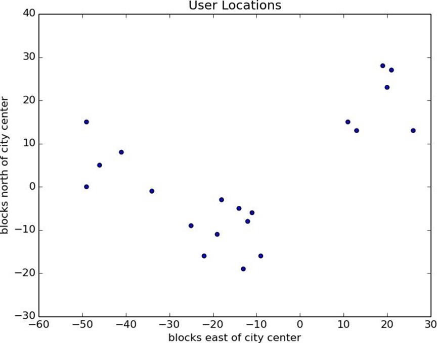
Figure 19-1. The locations of your hometown users
random.seed(0)clusterer=KMeans(2)
clusterer.train(inputs)clusterer.means
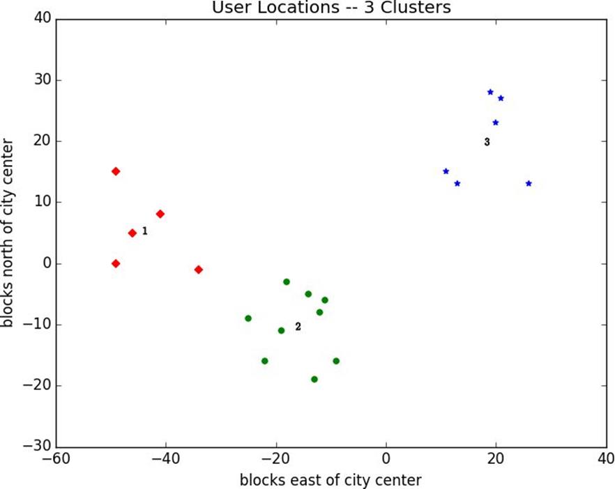
Figure 19-2. User locations grouped into three clusters
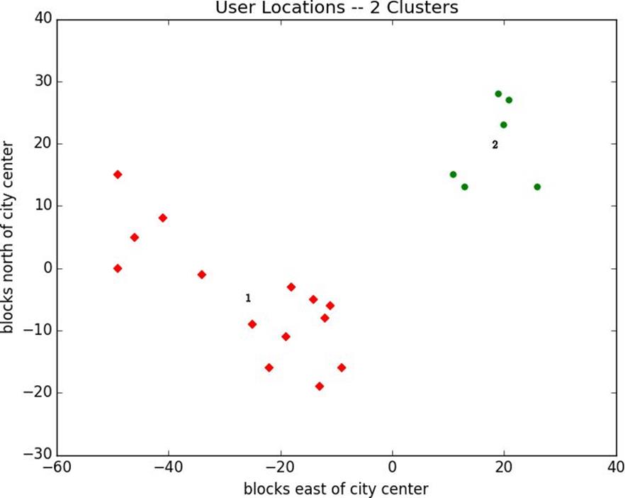
Figure 19-3. User locations grouped into two clusters
defsquared_clustering_errors(inputs,k):
"""finds the total squared error from k-means clustering the inputs"""
clusterer=KMeans(k)
clusterer.train(inputs)
means=clusterer.means
assignments=map(clusterer.classify,inputs)
returnsum(squared_distance(input,means[cluster])
forinput,clusterinzip(inputs,assignments))
# now plot from 1 up to len(inputs) clustersks=range(1,len(inputs)+1)
errors=[squared_clustering_errors(inputs,k)forkinks]
plt.plot(ks,errors)
plt.xticks(ks)plt.xlabel("k")plt.ylabel("total squared error")plt.title("Total Error vs. # of Clusters")plt.show()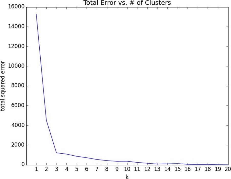
Figure 19-4. Choosing a k
Example: Clustering Colors
1. Choosing five colors
2. Assigning one of those colors to each pixel
path_to_png_file=r"C:\images\image.png"# wherever your image is
importmatplotlib.imageasmpimg
img=mpimg.imread(path_to_png_file)
top_row=img[0]
top_left_pixel=top_row[0]
red,green,blue=top_left_pixel
pixels=[pixelforrowinimgforpixelinrow]
clusterer=KMeans(5)
clusterer.train(pixels)# this might take a while
defrecolor(pixel):
cluster=clusterer.classify(pixel)# index of the closest cluster
returnclusterer.means[cluster]# mean of the closest cluster
new_img=[[recolor(pixel)forpixelinrow]# recolor this row of pixels
forrowinimg]# for each row in the image
plt.imshow(new_img)plt.axis('off')plt.show()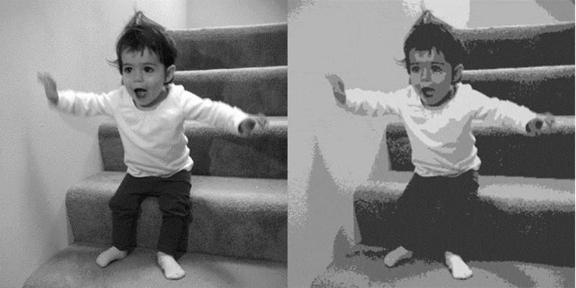
Figure 19-5. Original picture and its 5-means decoloring
1. Make each input its own cluster of one.
2. As long as there are multiple clusters remaining, find the two closest clusters and merge them.
leaf1=([10,20],)# to make a 1-tuple you need the trailing comma
leaf2=([30,-15],)# otherwise Python treats the parentheses as parentheses
merged=(1,[leaf1,leaf2])
defis_leaf(cluster):
"""a cluster is a leaf if it has length 1"""
returnlen(cluster)==1
defget_children(cluster):
"""returns the two children of this cluster if it's a merged cluster;
raises an exception if this is a leaf cluster"""ifis_leaf(cluster):
raiseTypeError("a leaf cluster has no children")
else:
returncluster[1]
defget_values(cluster):
"""returns the value in this cluster (if it's a leaf cluster)
or all the values in the leaf clusters below it (if it's not)"""ifis_leaf(cluster):
returncluster# is already a 1-tuple containing value
else:
return[value
forchildinget_children(cluster)
forvalueinget_values(child)]
defcluster_distance(cluster1,cluster2,distance_agg=min):
"""compute all the pairwise distances between cluster1 and cluster2
and apply _distance_agg_ to the resulting list"""returndistance_agg([distance(input1,input2)
forinput1inget_values(cluster1)
forinput2inget_values(cluster2)])
defget_merge_order(cluster):
ifis_leaf(cluster):
returnfloat('inf')
else:
returncluster[0]# merge_order is first element of 2-tuple
defbottom_up_cluster(inputs,distance_agg=min):
# start with every input a leaf cluster / 1-tuple
clusters=[(input,)forinputininputs]
# as long as we have more than one cluster left...
whilelen(clusters)>1:
# find the two closest clusters
c1,c2=min([(cluster1,cluster2)
fori,cluster1inenumerate(clusters)
forcluster2inclusters[:i]],
key=lambda(x,y):cluster_distance(x,y,distance_agg))
# remove them from the list of clusters
clusters=[cforcinclustersifc!=c1andc!=c2]
# merge them, using merge_order = # of clusters left
merged_cluster=(len(clusters),[c1,c2])
# and add their merge
clusters.append(merged_cluster)
# when there's only one cluster left, return it
returnclusters[0]
base_cluster=bottom_up_cluster(inputs)
(0, [(1, [(3, [(14, [(18, [([19, 28],),
([21, 27],)]),
([20, 23],)]),
([26, 13],)]),
(16, [([11, 15],),
([13, 13],)])]),
(2, [(4, [(5, [(9, [(11, [([-49, 0],),
([-46, 5],)]),
([-41, 8],)]),
([-49, 15],)]),
([-34, -1],)]),
(6, [(7, [(8, [(10, [([-22, -16],),
([-19, -11],)]),
([-25, -9],)]),
(13, [(15, [(17, [([-11, -6],),
([-12, -8],)]),
([-14, -5],)]),
([-18, -3],)])]),
(12, [([-13, -19],),
([-9, -16],)])])])])
§ Cluster 0 is the merger of cluster 1 and cluster 2.
§ Cluster 1 is the merger of cluster 3 and cluster 16.
§ Cluster 16 is the merger of the leaf [11, 15] and the leaf [13, 13].
§ And so on…
defgenerate_clusters(base_cluster,num_clusters):
# start with a list with just the base cluster
clusters=[base_cluster]
# as long as we don't have enough clusters yet...
whilelen(clusters)<num_clusters:
# choose the last-merged of our clusters
next_cluster=min(clusters,key=get_merge_order)
# remove it from the list
clusters=[cforcinclustersifc!=next_cluster]
# and add its children to the list (i.e., unmerge it)
clusters.extend(get_children(next_cluster))
# once we have enough clusters...
returnclusters
three_clusters=[get_values(cluster)
forclusteringenerate_clusters(base_cluster,3)]
fori,cluster,marker,colorinzip([1,2,3],
three_clusters,
['D','o','*'],
['r','g','b']):
xs,ys=zip(*cluster)# magic unzipping trick
plt.scatter(xs,ys,color=color,marker=marker)
# put a number at the mean of the cluster
x,y=vector_mean(cluster)
plt.plot(x,y,marker='$'+str(i)+'$',color='black')
plt.title("User Locations -- 3 Bottom-Up Clusters, Min")plt.xlabel("blocks east of city center")plt.ylabel("blocks north of city center")plt.show()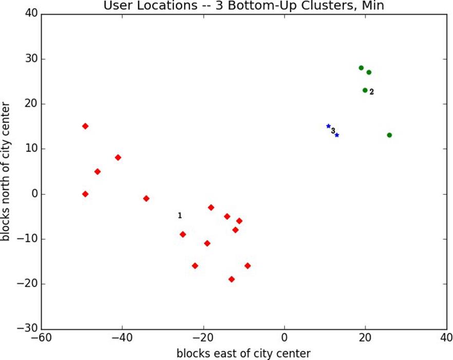
Figure 19-6. Three bottom-up clusters using min distance
NOTE
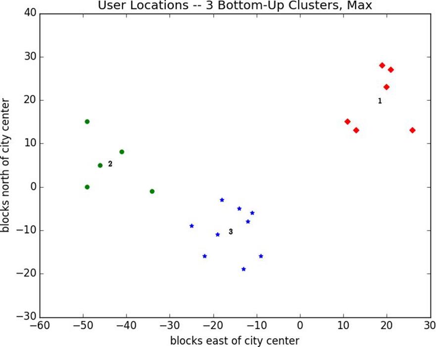
Figure 19-7. Three bottom-up clusters using max distance
§ scikit-learn has an entire module sklearn.cluster that contains several clustering algorithms including KMeans and the Ward hierarchical clustering algorithm (which uses a different criterion for merging clusters than ours did).
§ SciPy has two clustering models scipy.cluster.vq (which does k-means) and scipy.cluster.hierarchy (which has a variety of hierarchical clustering algorithms).