Network Analysis - Data Science from Scratch: First Principles with Python (2015)
Data Science from Scratch: First Principles with Python (2015)
Chapter 21.Network Analysis
Your connections to all the things around you literally define who you are.
Aaron O’Connell
Many interesting dataproblems can be fruitfully thought of interms ofnetworks, consisting ofnodesof some type and theedgesthat join them.
For instance, your Facebook friends form the nodes of a network whose edges are friendship relations. A less obvious example is the World Wide Web itself, with each web page a node, and each hyperlink from one page to another an edge.
Facebook friendship is mutual — if I am Facebook friends with you than necessarily you are friends with me. In this case, we say that the edges areundirected. Hyperlinks are not — my website links to whitehouse.gov, but (for reasons inexplicable to me) whitehouse.gov refuses to link to my website. We call these types of edgesdirected. We’ll look at both kinds of networks.
Betweenness Centrality
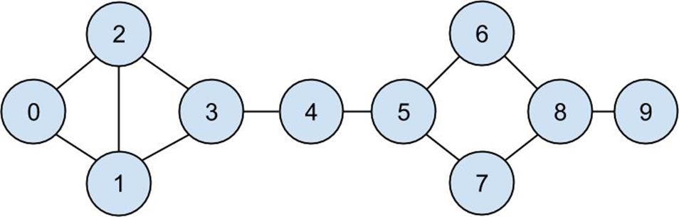
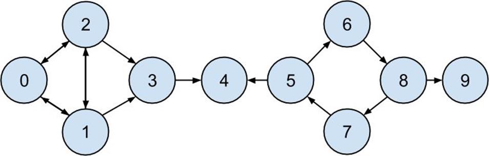
InChapter 1, we computed the key connectors in the DataSciencester network by counting the number of friends each user had.Now we have enough machinery to look at other approaches. Recall that the network (Figure 21-1) comprised users:
users=[
{"id":0,"name":"Hero"},
{"id":1,"name":"Dunn"},
{"id":2,"name":"Sue"},
{"id":3,"name":"Chi"},
{"id":4,"name":"Thor"},
{"id":5,"name":"Clive"},
{"id":6,"name":"Hicks"},
{"id":7,"name":"Devin"},
{"id":8,"name":"Kate"},
{"id":9,"name":"Klein"}
]
and friendships:
friendships=[(0,1),(0,2),(1,2),(1,3),(2,3),(3,4),
(4,5),(5,6),(5,7),(6,8),(7,8),(8,9)]
Figure 21-1.The DataSciencester network
We also added friend lists to each userdict:
foruserinusers:
user["friends"]=[]
fori,jinfriendships:
# this works because users[i] is the user whose id is i
users[i]["friends"].append(users[j])# add i as a friend of j
users[j]["friends"].append(users[i])# add j as a friend of i
When we left off we were dissatisfiedwith our notion ofdegree centrality, which didn’t really agree with our intuition about who were the key connectors of the network.
An alternative metric isbetweenness centrality, whichidentifies people who frequently are on the shortest paths between pairs of other people. In particular, the betweenness centrality of nodeiis computed by adding up, for every other pair of nodesjandk, the proportion of shortest paths between nodejand nodekthat pass throughi.
That is, to figure out Thor’s betweenness centrality, we’ll need to compute all the shortest paths between all pairs of people who aren’t Thor. And then we’ll need to count how many of those shortest paths pass through Thor. For instance, the only shortest path between Chi (id3) and Clive (id5) passes through Thor, while neither of the two shortest paths between Hero (id0) and Chi (id3) does.
So, as a first step, we’ll need to figure out the shortest paths between all pairs of people. There are some pretty sophisticated algorithms for doing so efficiently, but (as is almost always the case) we will use a less efficient, easier-to-understand algorithm.
This algorithm (an implementation of breadth-first search) is one of the more complicated ones in the book, so let’s talk through it carefully:
1. Our goal is a function that takes afrom_userand findsallshortest paths to every other user.
2. We’ll represent a path aslistof user IDs. Since every path starts atfrom_user, we won’t include her ID in the list. This means that the length of the list representing the path will be the length of the path itself.
3. We’ll maintain a dictionaryshortest_paths_towhere the keys are user IDs and the values are lists of paths that end at the user with the specified ID. If there is a unique shortest path, the list will just contain that one path. If there are multiple shortest paths, the list will contain all of them.
4. We’ll also maintain a queuefrontierthat contains the users we want to explore in the order we want to explore them. We’ll store them as pairs(prev_user, user)so that we know how we got to each one. We initialize the queue with all the neighbors offrom_user. (We haven’t ever talked about queues, which are data structures optimized for “add to the end” and “remove from the front” operations. In Python, they are implemented ascollections.dequewhich is actually a double-ended queue.)
5. As we explore the graph, whenever we find new neighbors that we don’t already know shortest paths to, we add them to the end of the queue to explore later, with the current user asprev_user.
6. When we take a user off the queue, and we’ve never encountered that user before, we’ve definitely found one or more shortest paths to him — each of the shortest paths toprev_userwith one extra step added.
7. When we take a user off the queue and wehaveencountered that user before, then either we’ve found another shortest path (in which case we should add it) or we’ve found a longer path (in which case we shouldn’t).
8. When no more users are left on the queue, we’ve explored the whole graph (or, at least, the parts of it that are reachable from the starting user) and we’re done.
We can put this all together into a (large) function:
fromcollectionsimportdeque
defshortest_paths_from(from_user):
# a dictionary from "user_id" to *all* shortest paths to that user
shortest_paths_to={from_user["id"]:[[]]}
# a queue of (previous user, next user) that we need to check.
# starts out with all pairs (from_user, friend_of_from_user)
frontier=deque((from_user,friend)
forfriendinfrom_user["friends"])
# keep going until we empty the queue
whilefrontier:
prev_user,user=frontier.popleft()# remove the user who's
user_id=user["id"]# first in the queue
# because of the way we're adding to the queue,
# necessarily we already know some shortest paths to prev_user
And we’re finally ready to compute betweenness centrality. For every pair of nodesiandj, we know thenshortest paths fromitoj. Then, for each of those paths, we just add1/nto the centrality of each node on that path:
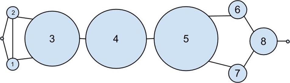
Figure 21-2.The DataSciencester network sized by betweenness centrality
As shown inFigure 21-2, users 0 and 9 have centrality 0 (as neither is on any shortest path between other users), whereas 3, 4, and 5 all have high centralities (as all three lie on many shortest paths).
NOTE
Generally the centrality numbers aren’t that meaningful themselves. What we care about is how the numbers for each node compare to the numbers for other nodes.
Another measure we can look at iscloseness centrality.First, for each user we compute herfarness, which is the sum of the lengths of her shortest paths to each other user. Since we’ve already computed the shortest paths between each pair of nodes, it’s easy to add their lengths. (If there are multiple shortest paths, they all have the same length, so we can just look at the first one.)
deffarness(user):
"""the sum of the lengths of the shortest paths to each other user"""
returnsum(len(paths[0])
forpathsinuser["shortest_paths"].values())
after which it’s very little work to compute closeness centrality (Figure 21-3):
foruserinusers:
user["closeness_centrality"]=1/farness(user)
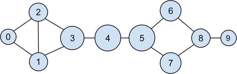
Figure 21-3.The DataSciencester network sized by closeness centrality
There is much less variation here — even the very central nodes are still pretty far from the nodes out on the periphery.
As we saw, computing shortest paths is kind of a pain. For this reason, betweenness and closeness centrality aren’t often used on large networks. The less intuitive (but generally easier to compute)eigenvector centralityis more frequently used.
Eigenvector Centrality
In order totalk about eigenvector centrality, we have to talk about eigenvectors, and in order to talk about eigenvectors, we have to talk about matrix multiplication.
Matrix Multiplication
IfAisamatrix andBis amatrix, and if, then their productABis thematrix whose (i,j)th entry is:
Which isjust thedotproduct of theith row ofA(thought of as a vector) with thejth column ofB(also thought of as a vector):
Notice that ifAis amatrix andBis amatrix, thenABis amatrix. If we treat a vector as a one-column matrix, we can think ofAas a function that mapsk-dimensional vectors ton-dimensional vectors, where the function is just matrix multiplication.
Previously we represented vectors simply as lists, which isn’t quite the same:
v=[1,2,3]
v_as_matrix=[[1],
[2],
[3]]
So we’ll need some helper functions to convert back and forth between the two representations:
defvector_as_matrix(v):
"""returns the vector v (represented as a list) as a n x 1 matrix"""
return[[v_i]forv_iinv]
defvector_from_matrix(v_as_matrix):
"""returns the n x 1 matrix as a list of values"""
return[row[0]forrowinv_as_matrix]
after which we can define the matrix operation usingmatrix_multiply:
defmatrix_operate(A,v):
v_as_matrix=vector_as_matrix(v)
product=matrix_multiply(A,v_as_matrix)
returnvector_from_matrix(product)
WhenAis asquarematrix, this operation mapsn-dimensional vectors to othern-dimensional vectors. It’s possible that, for some matrixAand vectorv, whenAoperates onvwe get back a scalar multiple ofv. That is, that the result is a vector that points in the same direction asv. When this happens (and when, in addition,vis not a vector of all zeroes), we callvaneigenvectorofA. And we call the multiplier aneigenvalue.
One possible way to find an eigenvector ofAis by picking a starting vectorv, applyingmatrix_operate, rescaling the result to have magnitude 1, and repeating until the process converges:
deffind_eigenvector(A,tolerance=0.00001):
guess=[random.random()for__inA]
whileTrue:
result=matrix_operate(A,guess)
length=magnitude(result)
next_guess=scalar_multiply(1/length,result)
ifdistance(guess,next_guess)<tolerance:
returnnext_guess,length# eigenvector, eigenvalue
guess=next_guess
By construction, the returnedguessis a vector such that, when you applymatrix_operateto it and rescale it to have length 1, you get back (a vector very close to) itself. Which means it’s an eigenvector.
Not all matrices of real numbers have eigenvectors and eigenvalues. For example the matrix:
rotate=[[0,1],
[-1,0]]
rotates vectors 90 degrees clockwise, which means that the only vector it maps to a scalar multiple of itself is a vector of zeroes. If you triedfind_eigenvector(rotate)it would run forever. Even matrices that have eigenvectors can sometimes get stuck in cycles. Consider the matrix:
flip=[[0,1],
[1,0]]
This matrix maps any vector[x, y]to[y, x]. This means that, for example,[1, 1]is an eigenvector with eigenvalue 1. However, if you start with a random vector with unequal coordinates,find_eigenvectorwill just repeatedly swap the coordinates forever. (Not-from-scratch libraries like NumPy use different methods that would work in this case.) Nonetheless, whenfind_eigenvectordoes return a result, that result is indeed an eigenvector.
Centrality
How does this help us understand the DataSciencester network?
To start with, we’ll need to represent the connections in our network as anadjacency_matrix, whose (i,j)th entry is either 1 (if useriand userjare friends) or 0 (if they’re not):
The eigenvector centrality for each user is then the entry corresponding to that user in the eigenvector returned byfind_eigenvector(Figure 21-4):
NOTE
For technical reasons that are way beyond the scope of this book, any nonzero adjacency matrix necessarily has an eigenvector all of whose values are non-negative. And fortunately for us, for thisadjacency_matrixourfind_eigenvectorfunction finds it.
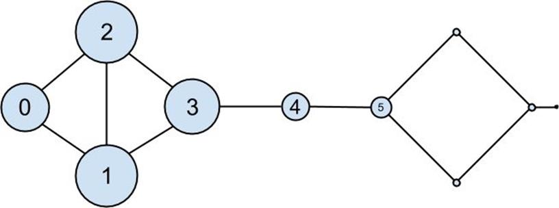
Figure 21-4.The DataSciencester network sized by eigenvector centrality
Users with high eigenvector centrality should be those who have a lot of connections and connections to people who themselves have high centrality.
Here users 1 and 2 are the most central, as they both have three connections to people who are themselves highly central. As we move away from them, people’s centralities steadily drop off.
On a network this small, eigenvector centrality behaves somewhat erratically. If you try adding or subtracting links, you’ll find that small changes in the network can dramatically change the centrality numbers. In a much larger network this would not particularly be the case.
We still haven’t motivated why an eigenvector might lead to a reasonable notion of centrality. Being an eigenvector means that if you compute:
which is precisely the sum of the eigenvector centralities of the users connected to useri.
In other words, eigenvector centralities are numbers, one per user, such that each user’s value is a constant multiple of the sum of his neighbors’ values. In this case centrality means being connected to people who themselves are central. The more centrality you are directly connected to, the more central you are. This is of course a circular definition — eigenvectors are the way of breaking out of the circularity.
Another way of understanding this is by thinking about whatfind_eigenvectoris doing here. It starts by assigning each node a random centrality. It then repeats the following two steps until the process converges:
1. Give each node a new centrality score that equals the sum of its neighbors’ (old) centrality scores.
2. Rescale the vector of centralities to have magnitude 1.
Although the mathematics behind it may seem somewhat opaque at first, the calculation itself is relatively straightforward (unlike, say, betweenness centrality) and is pretty easy to perform on even very large graphs.
Directed Graphs and PageRank
DataSciencester isn’t getting much traction, sothe VP of Revenue considers pivoting from a friendship model to an endorsement model. It turns out that no one particularly cares which data scientists arefriendswith one another, but tech recruiters care very much which data scientists are respected by other data scientists.
In this new model, we’ll track endorsements(source, target)that no longer represent a reciprocal relationship, but rather thatsourceendorsestargetas an awesome data scientist (Figure 21-5). We’ll need to account for this asymmetry:
endorsements=[(0,1),(1,0),(0,2),(2,0),(1,2),
(2,1),(1,3),(2,3),(3,4),(5,4),
(5,6),(7,5),(6,8),(8,7),(8,9)]
foruserinusers:
user["endorses"]=[]# add one list to track outgoing endorsements
user["endorsed_by"]=[]# and another to track endorsements
However, “number of endorsements” is an easy metric to game. All you need to do is create phony accounts and have them endorse you. Or arrange with your friends to endorse each other. (As users 0, 1, and 2 seem to have done.)
A better metric would take into accountwhoendorses you. Endorsements from people who have a lot of endorsements should somehow count more than endorsements from people with few endorsements.This is the essence of the PageRank algorithm, used by Google to rank websites based on which other websites link to them, which other websites link to those, and so on.
(If this sort of reminds you of the idea behind eigenvector centrality, it should.)
A simplified version looks like this:
1. There is a total of 1.0 (or 100%) PageRank in the network.
2. Initially this PageRank is equally distributed among nodes.
3. At each step, a large fraction of each node’s PageRank is distributed evenly among its outgoing links.
4. At each step, the remainder of each node’s PageRank is distributed evenly among all nodes.
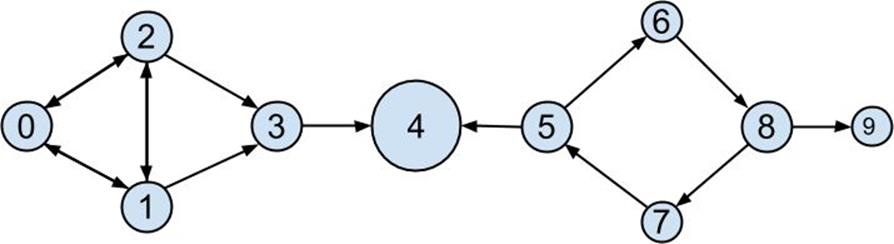
PageRank (Figure 21-6) identifies user 4 (Thor) as the highest ranked data scientist.
Figure 21-6.The DataSciencester network sized by PageRank
Even though he has fewer endorsements (2) than users 0, 1, and 2, his endorsements carry with them rank from their endorsements. Additionally, both of his endorsers endorsed only him, which means that he doesn’t have to divide their rank with anyone else.
For Further Exploration
§ There aremany other notions of centralitybesides the ones we used (although the ones we used are pretty much the most popular ones).
§ NetworkXis a Python library for network analysis. It has functions for computing centralities and for visualizing graphs.
§ Gephiis a love-it/hate-it GUI-based network-visualization tool.