Data Science from Scratch: First Principles with Python (2015)

Chapter 20. Natural Language Processing

They have been at a great feast of languages, and stolen the scraps.

William Shakespeare

Natural language processing (NLP) refers to computational techniques involving language. It’s a broad field, but we’ll look at a few techniques both simple and not simple.

In Chapter 1, we computed word counts of users’ interests. One approach to visualizing words and counts is word clouds, which artistically lay out the words with sizes proportional to their counts.

Generally, though, data scientists don’t think much of word clouds, in large part because the placement of the words doesn’t mean anything other than “here’s some space where I was able to fit a word.”

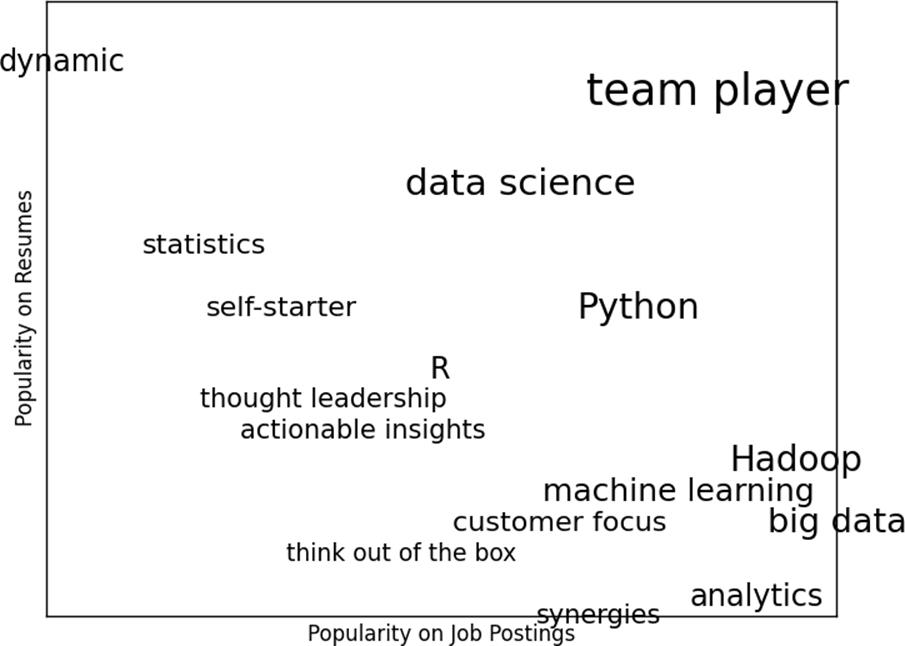
If you ever are forced to create a word cloud, think about whether you can make the axes convey something. For example, imagine that, for each of some collection of data science-related buzzwords, you have two numbers between 0 and 100 — the first representing how frequently it appears in job postings, the second how frequently it appears on resumes:

data = [ ("big data", 100, 15), ("Hadoop", 95, 25), ("Python", 75, 50),

         ("R", 50, 40), ("machine learning", 80, 20), ("statistics", 20, 60),

         ("data science", 60, 70), ("analytics", 90, 3),

         ("team player", 85, 85), ("dynamic", 2, 90), ("synergies", 70, 0),

         ("actionable insights", 40, 30), ("think out of the box", 45, 10),

         ("self-starter", 30, 50), ("customer focus", 65, 15),

         ("thought leadership", 35, 35)]

The word cloud approach is just to arrange the words on a page in a cool-looking font (Figure 20-1).

This looks neat but doesn’t really tell us anything. A more interesting approach might be to scatter them so that horizontal position indicates posting popularity and vertical position indicates resume popularity, which produces a visualization that conveys a few insights (Figure 20-2):

def text_size(total):

    """equals 8 if total is 0, 28 if total is 200"""

    return 8 + total / 200 * 20

for word, job_popularity, resume_popularity in data:

    plt.text(job_popularity, resume_popularity, word,

             ha='center', va='center',

             size=text_size(job_popularity + resume_popularity))

plt.xlabel("Popularity on Job Postings")

plt.ylabel("Popularity on Resumes")

plt.axis([0, 100, 0, 100])

plt.xticks([])

plt.yticks([])

plt.show()

The DataSciencester VP of Search Engine Marketing wants to create thousands of web pages about data science so that your site will rank higher in search results for data science-related terms. (You attempt to explain to her that search engine algorithms are clever enough that this won’t actually work, but she refuses to listen.)

Of course, she doesn’t want to write thousands of web pages, nor does she want to pay a horde of “content strategists” to do so. Instead she asks you whether you can somehow programatically generate these web pages. To do this, we’ll need some way of modeling language.

One approach is to start with a corpus of documents and learn a statistical model of language. In our case, we’ll start with Mike Loukides’s essay “What is data science?”

As in Chapter 9, we’ll use requests and BeautifulSoup to retrieve the data. There are a couple of issues worth calling attention to.

The first is that the apostrophes in the text are actually the Unicode character u"\u2019". We’ll create a helper function to replace them with normal apostrophes:

def fix_unicode(text):

    return text.replace(u"\u2019", "'")

The second issue is that once we get the text of the web page, we’ll want to split it into a sequence of words and periods (so that we can tell where sentences end). We can do this using re.findall():

from bs4 import BeautifulSoup

import requests

url = "http://radar.oreilly.com/2010/06/what-is-data-science.html"

html = requests.get(url).text

soup = BeautifulSoup(html, 'html5lib')

content = soup.find("div", "entry-content")   # find entry-content div

regex = r"[\w']+|[\.]"                        # matches a word or a period

document = []

for paragraph in content("p"):

    words = re.findall(regex, fix_unicode(paragraph.text))

    document.extend(words)

We certainly could (and likely should) clean this data further. There is still some amount of extraneous text in the document (for example, the first word is “Section”), and we’ve split on midsentence periods (for example, in “Web 2.0”), and there are a handful of captions and lists sprinkled throughout. Having said that, we’ll work with the document as it is.

Now that we have the text as a sequence of words, we can model language in the following way: given some starting word (say “book”) we look at all the words that follow it in the source documents (here “isn’t,” “a,” “shows,” “demonstrates,” and “teaches”). We randomly choose one of these to be the next word, and we repeat the process until we get to a period, which signifies the end of the sentence. We call this a bigram model, as it is determined completely by the frequencies of the bigrams (word pairs) in the original data.

What about a starting word? We can just pick randomly from words that follow a period. To start, let’s precompute the possible word transitions. Recall that zip stops when any of its inputs is done, so that zip(document, document[1:]) gives us precisely the pairs of consecutive elements ofdocument:

bigrams = zip(document, document[1:])

transitions = defaultdict(list)

for prev, current in bigrams:

    transitions[prev].append(current)

Now we’re ready to generate sentences:

def generate_using_bigrams():

    current = "."   # this means the next word will start a sentence

    result = []

    while True:

        next_word_candidates = transitions[current]    # bigrams (current, _)

        current = random.choice(next_word_candidates)  # choose one at random

        result.append(current)                         # append it to results

        if current == ".": return " ".join(result)     # if "." we're done

The sentences it produces are gibberish, but they’re the kind of gibberish you might put on your website if you were trying to sound data-sciencey. For example:

If you may know which are you want to data sort the data feeds web friend someone on trending topics as the data in Hadoop is the data science requires a book demonstrates why visualizations are but we do massive correlations across many commercial disk drives in Python language and creates more tractable form making connections then use and uses it to solve a data.

Bigram Model

We can make the sentences less gibberishy by looking at trigrams, triplets of consecutive words. (More generally, you might look at n-grams consisting of n consecutive words, but three will be plenty for us.) Now the transitions will depend on the previous two words:

trigrams = zip(document, document[1:], document[2:])

trigram_transitions = defaultdict(list)

starts = []

for prev, current, next in trigrams:

    if prev == ".":              # if the previous "word" was a period

        starts.append(current)   # then this is a start word

    trigram_transitions[(prev, current)].append(next)

Notice that now we have to track the starting words separately. We can generate sentences in pretty much the same way:

def generate_using_trigrams():

    current = random.choice(starts)   # choose a random starting word

    prev = "."                        # and precede it with a '.'

    result = [current]

    while True:

        next_word_candidates = trigram_transitions[(prev, current)]

        next_word = random.choice(next_word_candidates)

        prev, current = current, next_word

        result.append(current)

        if current == ".":

            return " ".join(result)

This produces better sentences like:

In hindsight MapReduce seems like an epidemic and if so does that give us new insights into how economies work That’s not a question we could even have asked a few years there has been instrumented.

Trigram Model

Of course, they sound better because at each step the generation process has fewer choices, and at many steps only a single choice. This means that you frequently generate sentences (or at least long phrases) that were seen verbatim in the original data. Having more data would help; it would also work better if you collected n-grams from multiple essays about data science.

A different approach to modeling language is with grammars, rules for generating acceptable sentences. In elementary school, you probably learned about parts of speech and how to combine them. For example, if you had a really bad English teacher, you might say that a sentence necessarily consists of a noun followed by a verb. If you then have a list of nouns and verbs, you can generate sentences according to the rule.

We’ll define a slightly more complicated grammar:

grammar = {

    "_S"  : ["_NP _VP"],

    "_NP" : ["_N",

             "_A _NP _P _A _N"],

    "_VP" : ["_V",

             "_V _NP"],

    "_N"  : ["data science", "Python", "regression"],

    "_A"  : ["big", "linear", "logistic"],

    "_P"  : ["about", "near"],

    "_V"  : ["learns", "trains", "tests", "is"]

}

I made up the convention that names starting with underscores refer to rules that need further expanding, and that other names are terminals that don’t need further processing.

So, for example, "_S" is the “sentence” rule, which produces a "_NP" (“noun phrase”) rule followed by a "_VP" (“verb phrase”) rule.

The verb phrase rule can produce either the "_V" (“verb”) rule, or the verb rule followed by the noun phrase rule.

Notice that the "_NP" rule contains itself in one of its productions. Grammars can be recursive, which allows even finite grammars like this to generate infinitely many different sentences.

How do we generate sentences from this grammar? We’ll start with a list containing the sentence rule ["_S"]. And then we’ll repeatedly expand each rule by replacing it with a randomly chosen one of its productions. We stop when we have a list consisting solely of terminals.

For example, one such progression might look like:

['_S']

['_NP','_VP']

['_N','_VP']

['Python','_VP']

['Python','_V','_NP']

['Python','trains','_NP']

['Python','trains','_A','_NP','_P','_A','_N']

['Python','trains','logistic','_NP','_P','_A','_N']

['Python','trains','logistic','_N','_P','_A','_N']

['Python','trains','logistic','data science','_P','_A','_N']

['Python','trains','logistic','data science','about','_A', '_N']

['Python','trains','logistic','data science','about','logistic','_N']

['Python','trains','logistic','data science','about','logistic','Python']

How do we implement this? Well, to start, we’ll create a simple helper function to identify terminals:

def is_terminal(token):

    return token[0] != "_"

Next we need to write a function to turn a list of tokens into a sentence. We’ll look for the first nonterminal token. If we can’t find one, that means we have a completed sentence and we’re done.

If we do find a nonterminal, then we randomly choose one of its productions. If that production is a terminal (i.e., a word), we simply replace the token with it. Otherwise it’s a sequence of space-separated nonterminal tokens that we need to split and then splice into the current tokens. Either way, we repeat the process on the new set of tokens.

Putting it all together we get:

def expand(grammar, tokens):

    for i, token in enumerate(tokens):

        # skip over terminals

        if is_terminal(token): continue

        # if we get here, we found a non-terminal token

        # so we need to choose a replacement at random

        replacement = random.choice(grammar[token])

        if is_terminal(replacement):

            tokens[i] = replacement

        else:

            tokens = tokens[:i] + replacement.split() + tokens[(i+1):]

        # now call expand on the new list of tokens

        return expand(grammar, tokens)

    # if we get here we had all terminals and are done

    return tokens

And now we can start generating sentences:

def generate_sentence(grammar):

    return expand(grammar, ["_S"])

Try changing the grammar — add more words, add more rules, add your own parts of speech — until you’re ready to generate as many web pages as your company needs.

Grammars are actually more interesting when they’re used in the other direction. Given a sentence we can use a grammar to parse the sentence. This then allows us to identify subjects and verbs and helps us make sense of the sentence.

Using data science to generate text is a neat trick; using it to understand text is more magical. (See “For Further Investigation” for libraries that you could use for this.)

Generating samples from some distributions is easy. We can get uniform random variables with:

random.random()

and normal random variables with:

inverse_normal_cdf(random.random())

But some distributions are harder to sample from. Gibbs sampling is a technique for generating samples from multidimensional distributions when we only know some of the conditional distributions.

For example, imagine rolling two dice. Let x be the value of the first die and y be the sum of the dice, and imagine you wanted to generate lots of (x, y) pairs. In this case it’s easy to generate the samples directly:

def roll_a_die():

    return random.choice([1,2,3,4,5,6])

def direct_sample():

    d1 = roll_a_die()

    d2 = roll_a_die()

    return d1, d1 + d2

But imagine that you only knew the conditional distributions. The distribution of y conditional on x is easy — if you know the value of x, y is equally likely to be x + 1, x + 2, x + 3, x + 4, x + 5, or x + 6:

def random_y_given_x(x):

    """equally likely to be x + 1, x + 2, ... , x + 6"""

    return x + roll_a_die()

The other direction is more complicated. For example, if you know that y is 2, then necessarily x is 1 (since the only way two dice can sum to 2 is if both of them are 1). If you know y is 3, then x is equally likely to be 1 or 2. Similarly, if y is 11, then x has to be either 5 or 6:

def random_x_given_y(y):

    if y <= 7:

        # if the total is 7 or less, the first die is equally likely to be

        # 1, 2, ..., (total - 1)

        return random.randrange(1, y)

    else:

        # if the total is 7 or more, the first die is equally likely to be

        # (total - 6), (total - 5), ..., 6

        return random.randrange(y - 6, 7)

The way Gibbs sampling works is that we start with any (valid) value for x and y and then repeatedly alternate replacing x with a random value picked conditional on y and replacing y with a random value picked conditional on x. After a number of iterations, the resulting values of x and ywill represent a sample from the unconditional joint distribution:

def gibbs_sample(num_iters=100):

    x, y = 1, 2 # doesn't really matter

    for _ in range(num_iters):

        x = random_x_given_y(y)

        y = random_y_given_x(x)

    return x, y

You can check that this gives similar results to the direct sample:

def compare_distributions(num_samples=1000):

    counts = defaultdict(lambda: [0, 0])

    for _ in range(num_samples):

        counts[gibbs_sample()][0] += 1

        counts[direct_sample()][1] += 1

    return counts

We’ll use this technique in the next section.

When we built our Data Scientists You Should Know recommender in Chapter 1, we simply looked for exact matches in people’s stated interests.

A more sophisticated approach to understanding our users’ interests might try to identify the topics that underlie those interests. A technique called Latent Dirichlet Analysis (LDA) is commonly used to identify common topics in a set of documents. We’ll apply it to documents that consist of each user’s interests.

LDA has some similarities to the Naive Bayes Classifier we built in Chapter 13, in that it assumes a probabilistic model for documents. We’ll gloss over the hairier mathematical details, but for our purposes the model assumes that:

§ There is some fixed number K of topics.

§ There is a random variable that assigns each topic an associated probability distribution over words. You should think of this distribution as the probability of seeing word w given topic k.

§ There is another random variable that assigns each document a probability distribution over topics. You should think of this distribution as the mixture of topics in document d.

§ Each word in a document was generated by first randomly picking a topic (from the document’s distribution of topics) and then randomly picking a word (from the topic’s distribution of words).

In particular, we have a collection of documents each of which is a list of words. And we have a corresponding collection of document_topics that assigns a topic (here a number between 0 and K - 1) to each word in each document.

So that the fifth word in the fourth document is:

documents[3][4]

and the topic from which that word was chosen is:

document_topics[3][4]

This very explicitly defines each document’s distribution over topics, and it implicitly defines each topic’s distribution over words.

We can estimate the likelihood that topic 1 produces a certain word by comparing how many times topic 1 produces that word with how many times topic 1 produces any word. (Similarly, when we built a spam filter in Chapter 13, we compared how many times each word appeared in spams with the total number of words appearing in spams.)

Although these topics are just numbers, we can give them descriptive names by looking at the words on which they put the heaviest weight. We just have to somehow generate the document_topics. This is where Gibbs sampling comes into play.

We start by assigning every word in every document a topic completely at random. Now we go through each document one word at a time. For that word and document, we construct weights for each topic that depend on the (current) distribution of topics in that document and the (current) distribution of words for that topic. We then use those weights to sample a new topic for that word. If we iterate this process many times, we will end up with a joint sample from the topic-word distribution and the document-topic distribution.

To start with, we’ll need a function to randomly choose an index based on an arbitrary set of weights:

def sample_from(weights):

    """returns i with probability weights[i] / sum(weights)"""

    total = sum(weights)

    rnd = total * random.random()      # uniform between 0 and total

    for i, w in enumerate(weights):

        rnd -= w                       # return the smallest i such that

        if rnd <= 0: return i          # weights[0] + ... + weights[i] >= rnd

For instance, if you give it weights [1, 1, 3] then one-fifth of the time it will return 0, one-fifth of the time it will return 1, and three-fifths of the time it will return 2.

Our documents are our users’ interests, which look like:

documents = [

    ["Hadoop", "Big Data", "HBase", "Java", "Spark", "Storm", "Cassandra"],

    ["NoSQL", "MongoDB", "Cassandra", "HBase", "Postgres"],

    ["Python", "scikit-learn", "scipy", "numpy", "statsmodels", "pandas"],

    ["R", "Python", "statistics", "regression", "probability"],

    ["machine learning", "regression", "decision trees", "libsvm"],

    ["Python", "R", "Java", "C++", "Haskell", "programming languages"],

    ["statistics", "probability", "mathematics", "theory"],

    ["machine learning", "scikit-learn", "Mahout", "neural networks"],

    ["neural networks", "deep learning", "Big Data", "artificial intelligence"],

    ["Hadoop", "Java", "MapReduce", "Big Data"],

    ["statistics", "R", "statsmodels"],

    ["C++", "deep learning", "artificial intelligence", "probability"],

    ["pandas", "R", "Python"],

    ["databases", "HBase", "Postgres", "MySQL", "MongoDB"],

    ["libsvm", "regression", "support vector machines"]

]

And we’ll try to find K = 4 topics.

In order to calculate the sampling weights, we’ll need to keep track of several counts. Let’s first create the data structures for them.

How many times each topic is assigned to each document:

# a list of Counters, one for each document

document_topic_counts = [Counter() for _ in documents]

How many times each word is assigned to each topic:

# a list of Counters, one for each topic

topic_word_counts = [Counter() for _ in range(K)]

The total number of words assigned to each topic:

# a list of numbers, one for each topic

topic_counts = [0 for _ in range(K)]

The total number of words contained in each document:

# a list of numbers, one for each document

document_lengths = map(len, documents)

The number of distinct words:

distinct_words = set(word for document in documents for word in document)

W = len(distinct_words)

And the number of documents:

D = len(documents)

For example, once we populate these, we can find, for example, the number of words in documents[3] associated with topic 1 as:

document_topic_counts[3][1]

And we can find the number of times nlp is associated with topic 2 as:

topic_word_counts[2]["nlp"]

Now we’re ready to define our conditional probability functions. As in Chapter 13, each has a smoothing term that ensures every topic has a nonzero chance of being chosen in any document and that every word has a nonzero chance of being chosen for any topic:

def p_topic_given_document(topic, d, alpha=0.1):

    """the fraction of words in document _d_

    that are assigned to _topic_ (plus some smoothing)"""

    return ((document_topic_counts[d][topic] + alpha) /

            (document_lengths[d] + K * alpha))

def p_word_given_topic(word, topic, beta=0.1):

    """the fraction of words assigned to _topic_

    that equal _word_ (plus some smoothing)"""

    return ((topic_word_counts[topic][word] + beta) /

            (topic_counts[topic] + W * beta))

We’ll use these to create the weights for updating topics:

def topic_weight(d, word, k):

    """given a document and a word in that document,

    return the weight for the kth topic"""

    return p_word_given_topic(word, k) * p_topic_given_document(k, d)

def choose_new_topic(d, word):

    return sample_from([topic_weight(d, word, k)

                        for k in range(K)])

There are solid mathematical reasons why topic_weight is defined the way it is, but their details would lead us too far afield. Hopefully it makes at least intuitive sense that — given a word and its document — the likelihood of any topic choice depends on both how likely that topic is for the document and how likely that word is for the topic.

This is all the machinery we need. We start by assigning every word to a random topic, and populating our counters appropriately:

random.seed(0)

document_topics = [[random.randrange(K) for word in document]

                   for document in documents]

for d in range(D):

    for word, topic in zip(documents[d], document_topics[d]):

        document_topic_counts[d][topic] += 1

        topic_word_counts[topic][word] += 1

        topic_counts[topic] += 1

Our goal is to get a joint sample of the topics-words distribution and the documents-topics distribution. We do this using a form of Gibbs sampling that uses the conditional probabilities defined previously:

for iter in range(1000):

    for d in range(D):

        for i, (word, topic) in enumerate(zip(documents[d],

                                              document_topics[d])):

            # remove this word / topic from the counts

            # so that it doesn't influence the weights

            document_topic_counts[d][topic] -= 1

            topic_word_counts[topic][word] -= 1

            topic_counts[topic] -= 1

            document_lengths[d] -= 1

            # choose a new topic based on the weights

            new_topic = choose_new_topic(d, word)

            document_topics[d][i] = new_topic

            # and now add it back to the counts

            document_topic_counts[d][new_topic] += 1

            topic_word_counts[new_topic][word] += 1

            topic_counts[new_topic] += 1

            document_lengths[d] += 1

What are the topics? They’re just numbers 0, 1, 2, and 3. If we want names for them we have to do that ourselves. Let’s look at the five most heavily weighted words for each (Table 20-1):

for k, word_counts in enumerate(topic_word_counts):

    for word, count in word_counts.most_common():

        if count > 0: print k, word, count

Based on these I’d probably assign topic names:

topic_names = ["Big Data and programming languages",

               "Python and statistics",

               "databases",

               "machine learning"]

at which point we can see how the model assigns topics to each user’s interests:

for document, topic_counts in zip(documents, document_topic_counts):

    print document

    for topic, count in topic_counts.most_common():

        if count > 0:

            print topic_names[topic], count,

    print

which gives:

['Hadoop', 'Big Data', 'HBase', 'Java', 'Spark', 'Storm', 'Cassandra']

Big Data and programming languages 4 databases 3

['NoSQL', 'MongoDB', 'Cassandra', 'HBase', 'Postgres']

databases 5

['Python', 'scikit-learn', 'scipy', 'numpy', 'statsmodels', 'pandas']

Python and statistics 5 machine learning 1

and so on. Given the “ands” we needed in some of our topic names, it’s possible we should use more topics, although most likely we don’t have enough data to successfully learn them.

§ Natural Language Toolkit is a popular (and pretty comprehensive) library of NLP tools for Python. It has its own entire book, which is available to read online.

§ gensim is a Python library for topic modeling, which is a better bet than our from-scratch model.