Linear Algebra - Data Science from Scratch: First Principles with Python (2015)
Data Science from Scratch: First Principles with Python (2015)
Chapter 4.Linear Algebra
Is there anything more useless or less useful than Algebra?
Billy Connolly
Linear algebra is the branchof mathematics that deals withvector spaces. Although I can’t hope to teach you linear algebra in a brief chapter, it underpins a large number of data science concepts and techniques, which means I owe it to you to at least try. What we learn in this chapter we’ll use heavily throughout the rest of the book.
Vectors
Abstractly,vectorsare objects thatcan be added together (to form new vectors) and that can be multipliedbyscalars(i.e., numbers), also to form new vectors.
Concretely (for us), vectors are points in some finite-dimensional space. Although you might not think of your data as vectors, they are a good way to represent numeric data.
For example, if you have the heights, weights, and ages of a large number of people, you can treat your data as three-dimensional vectors(height, weight, age). If you’re teaching a class with four exams, you can treat student grades as four-dimensional vectors(exam1, exam2, exam3, exam4).
The simplest from-scratch approach is to represent vectors as lists of numbers.A list of three numbers corresponds to a vector in three-dimensional space, and vice versa:
height_weight_age=[70,# inches,
170,# pounds,
40]# years
grades=[95,# exam1
80,# exam2
75,# exam3
62]# exam4
One problem with this approach is that we will want to performarithmeticon vectors.Because Python lists aren’t vectors (and hence provide no facilities for vector arithmetic), we’ll need to build these arithmetic tools ourselves. So let’s start with that.
To begin with, we’ll frequently need to add two vectors. Vectors addcomponentwise.This means that if two vectorsvandware the same length, their sum is just the vector whose first element isv[0] + w[0], whose second element isv[1] + w[1], and so on. (If they’re not the same length, then we’re not allowed to add them.)
For example, adding the vectors[1, 2]and[2, 1]results in[1 + 2, 2 + 1]or[3, 3], as shown inFigure 4-1.
We can easily implement this byzip-ing the vectors together and using a list comprehensionto add the corresponding elements:
defvector_add(v,w):
"""adds corresponding elements"""
return[v_i+w_i
forv_i,w_iinzip(v,w)]
Similarly, to subtract two vectorswe just subtract corresponding elements:
defvector_subtract(v,w):
"""subtracts corresponding elements"""
return[v_i-w_i
forv_i,w_iinzip(v,w)]
We’ll also sometimes want to componentwise sum a list of vectors. That is, create a new vector whose first element is the sum of all the first elements, whose second element is the sum of all the second elements, and so on. The easiest way to do this is by adding one vector at a time:
defvector_sum(vectors):
"""sums all corresponding elements"""
result=vectors[0]# start with the first vector
forvectorinvectors[1:]:# then loop over the others
result=vector_add(result,vector)# and add them to the result
returnresult
If you think aboutit, we are justreduce-ing the list of vectors usingvector_add, which means we can rewrite this more briefly using higher-order functions:
defvector_sum(vectors):
returnreduce(vector_add,vectors)
or even:
vector_sum=partial(reduce,vector_add)
although this last one is probably more clever than helpful.
We’ll also need to be ableto multiply a vector by a scalar, which we do simply by multiplying each element of the vector by that number:
defscalar_multiply(c,v):
"""c is a number, v is a vector"""
return[c*v_iforv_iinv]
This allows us to compute the componentwise means of a list of (same-sized) vectors:
defvector_mean(vectors):
"""compute the vector whose ith element is the mean of the
ith elements of the input vectors"""
n=len(vectors)
returnscalar_multiply(1/n,vector_sum(vectors))
A less obvious tool is thedot product.The dot product of two vectors is the sum of their componentwise products:
defdot(v,w):
"""v_1 * w_1 + ... + v_n * w_n"""
returnsum(v_i*w_i
forv_i,w_iinzip(v,w))
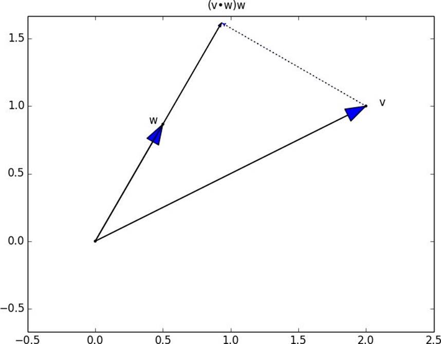
The dot product measures how far the vectorvextends in thewdirection. For example, ifw = [1, 0]thendot(v, w)is just the first component ofv. Another way of saying this is that it’s the length of the vector you’d get if youprojectedvontow(Figure 4-2).
Using this, it’s easy tocompute a vector’ssum of squares:
defsum_of_squares(v):
"""v_1 * v_1 + ... + v_n * v_n"""
returndot(v,v)
Which we can use tocompute itsmagnitude(or length):
importmath
defmagnitude(v):
returnmath.sqrt(sum_of_squares(v))# math.sqrt is square root function
We now have all the pieces we need tocompute the distance between two vectors, defined as:
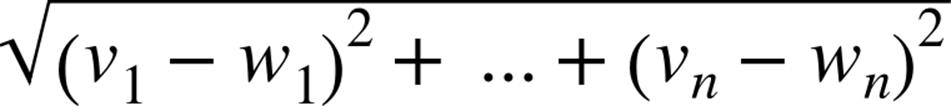
defsquared_distance(v,w):
"""(v_1 - w_1) ** 2 + ... + (v_n - w_n) ** 2"""
returnsum_of_squares(vector_subtract(v,w))
defdistance(v,w):
returnmath.sqrt(squared_distance(v,w))
Which is possibly clearer if we write it as (the equivalent):
defdistance(v,w):
returnmagnitude(vector_subtract(v,w))
That should be plenty to get us started. We’ll be using these functions heavily throughout the book.
NOTE
Using lists as vectors is great for exposition but terrible for performance.
In production code, you would want to use the NumPy library, which includes a high-performance array class with all sorts of arithmetic operations included.
Matrices
Amatrixis a two-dimensional collection of numbers.We will represent matrices aslists oflists, with each inner list having the same size and representing arowof the matrix.IfAis a matrix, thenA[i][j]is the element in theith row and thejth column. Per mathematical convention, we will typically use capital letters to represent matrices. For example:
A=[[1,2,3],# A has 2 rows and 3 columns
[4,5,6]]
B=[[1,2],# B has 3 rows and 2 columns
[3,4],
[5,6]]
NOTE
In mathematics, you would usually name the first row of the matrix “row 1” and the first column “column 1.” Because we’re representing matrices with Pythonlists, which are zero-indexed, we’ll call the first row of a matrix “row 0” and the first column “column 0.”
Given this list-of-lists representation, the matrixAhaslen(A)rows andlen(A[0])columns, which we consider itsshape:
defshape(A):
num_rows=len(A)
num_cols=len(A[0])ifAelse0# number of elements in first row
returnnum_rows,num_cols
If a matrix hasnrows andkcolumns, we will refer to it as amatrix. We can (and sometimes will) think of each row of amatrix as a vector of lengthk, and each column as a vector of lengthn:
defget_row(A,i):
returnA[i]# A[i] is already the ith row
defget_column(A,j):
return[A_i[j]# jth element of row A_i
forA_iinA]# for each row A_i
We’ll also want to be able to create a matrix given its shape and a function for generating its elements. We can do this using a nested list comprehension:
defmake_matrix(num_rows,num_cols,entry_fn):
"""returns a num_rows x num_cols matrix
whose (i,j)th entry is entry_fn(i, j)"""
return[[entry_fn(i,j)# given i, create a list
forjinrange(num_cols)]# [entry_fn(i, 0), ... ]
foriinrange(num_rows)]# create one list for each i
Given this function, you could make a 5 × 5identity matrix(with 1s on the diagonal and 0s elsewhere) with:
defis_diagonal(i,j):
"""1's on the 'diagonal', 0's everywhere else"""
return1ifi==jelse0
identity_matrix=make_matrix(5,5,is_diagonal)
# [[1, 0, 0, 0, 0],
# [0, 1, 0, 0, 0],
# [0, 0, 1, 0, 0],
# [0, 0, 0, 1, 0],
# [0, 0, 0, 0, 1]]
Matrices will be important to us for several reasons.
First, we can use a matrix to represent adata set consisting of multiple vectors, simply by considering each vector as a row of the matrix.For example, if you had the heights, weights, and ages of 1,000 people you could put them in amatrix:
data=[[70,170,40],
[65,120,26],
[77,250,19],
# ....
]
Second, as we’ll see later, we can use anmatrix to represent a linear function that mapsk-dimensional vectors ton-dimensional vectors. Several of our techniques and concepts will involve such functions.
Third, matrices can be used to represent binary relationships.InChapter 1, we represented the edges of a network as a collection of pairs(i, j). An alternative representation would be to create a matrixAsuch thatA[i][j]is 1 if nodesiandjare connected and 0 otherwise.
Recall that before we had:
friendships=[(0,1),(0,2),(1,2),(1,3),(2,3),(3,4),
(4,5),(5,6),(5,7),(6,8),(7,8),(8,9)]
We could also represent this as:
# user 0 1 2 3 4 5 6 7 8 9
#
friendships=[[0,1,1,0,0,0,0,0,0,0],# user 0
[1,0,1,1,0,0,0,0,0,0],# user 1
[1,1,0,1,0,0,0,0,0,0],# user 2
[0,1,1,0,1,0,0,0,0,0],# user 3
[0,0,0,1,0,1,0,0,0,0],# user 4
[0,0,0,0,1,0,1,1,0,0],# user 5
[0,0,0,0,0,1,0,0,1,0],# user 6
[0,0,0,0,0,1,0,0,1,0],# user 7
[0,0,0,0,0,0,1,1,0,1],# user 8
[0,0,0,0,0,0,0,0,1,0]]# user 9
If there are very few connections, this is a much more inefficient representation, since you end up having to store a lot of zeroes. However, with the matrix representation it is much quicker to check whether two nodes are connected — you just have to do a matrix lookup instead of (potentially) inspecting every edge:
friendships[0][2]==1# True, 0 and 2 are friends
friendships[0][8]==1# False, 0 and 8 are not friends
Similarly, to find the connections a node has, you only need to inspect the column (or the row) corresponding to that node:
friends_of_five=[i# only need
fori,is_friendinenumerate(friendships[5])# to look at
ifis_friend]# one row
Previously we added a list of connections to each node object to speed up this process, but for a large, evolving graph that would probably be too expensive and difficult to maintain.
We’ll revisit matrices throughout the book.
For Further Exploration
§ Linear algebra is widely used by data scientists (frequently implicitly, and not infrequently by people who don’t understand it). It wouldn’t be a bad idea to read a textbook. You can find several freely available online:
§ Linear Algebra, from UC Davis
§ Linear Algebra, from Saint Michael’s College
§ If you are feeling adventurous,Linear Algebra Done Wrongis a more advanced introduction
§ All of the machinery we built here you get for free if you useNumPy. (You get a lot more too.)