Data Science from Scratch: First Principles with Python (2015)
Chapter 8. Gradient Descent
Those who boast of their descent, brag on what they owe to others.
Seneca
The Idea Behind Gradient Descent
defsum_of_squares(v):
"""computes the sum of squared elements in v"""
returnsum(v_i**2forv_iinv)
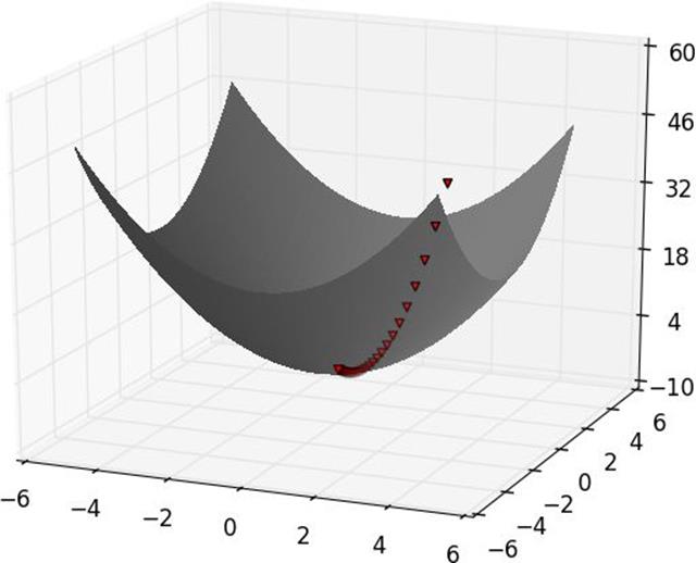
Figure 8-1. Finding a minimum using gradient descent
NOTE
defdifference_quotient(f,x,h):
return(f(x+h)-f(x))/h
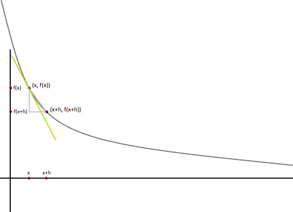
Figure 8-2. Approximating a derivative with a difference quotient
The derivative is the slope of the tangent line at 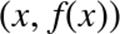 , while the difference quotient is the slope of the not-quite-tangent line that runs through
  . As h gets smaller and smaller, the not-quite-tangent line gets closer and closer to the tangent line (Figure 8-2).
defsquare(x):
returnx*x
defderivative(x):
return2*x
derivative_estimate=partial(difference_quotient,square,h=0.00001)
# plot to show they're basically the sameimportmatplotlib.pyplotasplt
x=range(-10,10)
plt.title("Actual Derivatives vs. Estimates")plt.plot(x,map(derivative,x),'rx',label='Actual')# red x
plt.plot(x,map(derivative_estimate,x),'b+',label='Estimate')# blue +
plt.legend(loc=9)plt.show()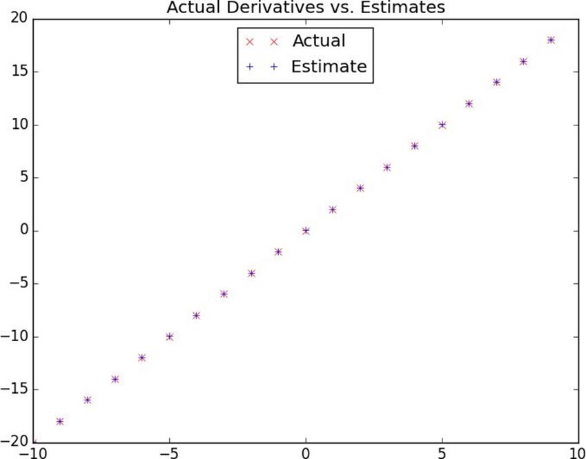
Figure 8-3. Goodness of difference quotient approximation
defpartial_difference_quotient(f,v,i,h):
"""compute the ith partial difference quotient of f at v"""
w=[v_j+(hifj==ielse0)# add h to just the ith element of v
forj,v_jinenumerate(v)]
return(f(w)-f(v))/h
defestimate_gradient(f,v,h=0.00001):
return[partial_difference_quotient(f,v,i,h)
fori,_inenumerate(v)]
NOTE
defstep(v,direction,step_size):
"""move step_size in the direction from v"""
return[v_i+step_size*direction_i
forv_i,direction_iinzip(v,direction)]
defsum_of_squares_gradient(v):
return[2*v_iforv_iinv]
# pick a random starting pointv=[random.randint(-10,10)foriinrange(3)]
tolerance=0.0000001
whileTrue:
gradient=sum_of_squares_gradient(v)# compute the gradient at v
next_v=step(v,gradient,-0.01)# take a negative gradient step
ifdistance(next_v,v)<tolerance:# stop if we're converging
break
v=next_v# continue if we're not
Choosing the Right Step Size
§ Using a fixed step size
§ Gradually shrinking the step size over time
§ At each step, choosing the step size that minimizes the value of the objective function
step_sizes=[100,10,1,0.1,0.01,0.001,0.0001,0.00001]
defsafe(f):
"""return a new function that's the same as f,
except that it outputs infinity whenever f produces an error"""defsafe_f(*args,**kwargs):
try:
returnf(*args,**kwargs)
except:
returnfloat('inf')# this means "infinity" in Python
returnsafe_f
Putting It All Together
defminimize_batch(target_fn,gradient_fn,theta_0,tolerance=0.000001):
"""use gradient descent to find theta that minimizes target function"""
step_sizes=[100,10,1,0.1,0.01,0.001,0.0001,0.00001]
theta=theta_0# set theta to initial value
target_fn=safe(target_fn)# safe version of target_fn
value=target_fn(theta)# value we're minimizing
whileTrue:
gradient=gradient_fn(theta)
next_thetas=[step(theta,gradient,-step_size)
forstep_sizeinstep_sizes]
# choose the one that minimizes the error function
next_theta=min(next_thetas,key=target_fn)
next_value=target_fn(next_theta)
# stop if we're "converging"
ifabs(value-next_value)<tolerance:
returntheta
else:
theta,value=next_theta,next_value
defnegate(f):
"""return a function that for any input x returns -f(x)"""
returnlambda*args,**kwargs:-f(*args,**kwargs)
defnegate_all(f):
"""the same when f returns a list of numbers"""
returnlambda*args,**kwargs:[-yforyinf(*args,**kwargs)]
defmaximize_batch(target_fn,gradient_fn,theta_0,tolerance=0.000001):
returnminimize_batch(negate(target_fn),
negate_all(gradient_fn),
theta_0,
tolerance)
Stochastic Gradient Descent
defin_random_order(data):
"""generator that returns the elements of data in random order"""
indexes=[ifori,_inenumerate(data)]# create a list of indexes
random.shuffle(indexes)# shuffle them
foriinindexes:# return the data in that order
yielddata[i]
defminimize_stochastic(target_fn,gradient_fn,x,y,theta_0,alpha_0=0.01):
data=zip(x,y)
theta=theta_0# initial guess
alpha=alpha_0# initial step size
min_theta,min_value=None,float("inf")# the minimum so far
iterations_with_no_improvement=0
# if we ever go 100 iterations with no improvement, stop
whileiterations_with_no_improvement<100:
value=sum(target_fn(x_i,y_i,theta)forx_i,y_iindata)
ifvalue<min_value:
# if we've found a new minimum, remember it
# and go back to the original step size
min_theta,min_value=theta,value
iterations_with_no_improvement=0
alpha=alpha_0
else:
# otherwise we're not improving, so try shrinking the step size
iterations_with_no_improvement+=1
alpha*=0.9
# and take a gradient step for each of the data points
forx_i,y_iinin_random_order(data):
gradient_i=gradient_fn(x_i,y_i,theta)
theta=vector_subtract(theta,scalar_multiply(alpha,gradient_i))
returnmin_theta
defmaximize_stochastic(target_fn,gradient_fn,x,y,theta_0,alpha_0=0.01):
returnminimize_stochastic(negate(target_fn),
negate_all(gradient_fn),
x,y,theta_0,alpha_0)
For Further Exploration
§ Keep reading! We’ll be using gradient descent to solve problems throughout the rest of the book.
§ At this point, you’re undoubtedly sick of me recommending that you read textbooks. If it’s any consolation, Active Calculus seems nicer than the calculus textbooks I learned from.
§ scikit-learn has a Stochastic Gradient Descent module that is not as general as ours in some ways and more general in other ways. Really, though, in most real-world situations you’ll be using libraries in which the optimization is already taken care of behind the scenes, and you won’t have to worry about it yourself (other than when it doesn’t work correctly, which one day, inevitably, it won’t).
All materials on the site are licensed Creative Commons Attribution-Sharealike 3.0 Unported CC BY-SA 3.0 & GNU Free Documentation License (GFDL)
If you are the copyright holder of any material contained on our site and intend to remove it, please contact our site administrator for approval.
© 2016-2026 All site design rights belong to S.Y.A.