Python Unlocked (2015)
Chapter 7. Optimization Techniques
In this chapter, we will learn how to optimize our Python code to get better responsive programs. But, before we dive into this, I would like to stress that do not optimize until it is necessary. A better-readable program has a better life and maintainability than a tersely-optimized program. First, we will take a look at simple optimization tricks to keep a program optimized. We should have knowledge about them so that we can apply easy optimizations from the start. Then, we will look at profiling to find bottlenecks in the current program and apply optimizations where we need them. As a last resort, we can compile in the C language and provide functionality as an extension to Python. Here is the gist of topics that we will cover:
· Writing optimized code
· Profiling to find bottlenecks
· Using fast libraries
· Using C speeds
Writing optimized code
Key 1: Easy optimizations for code.
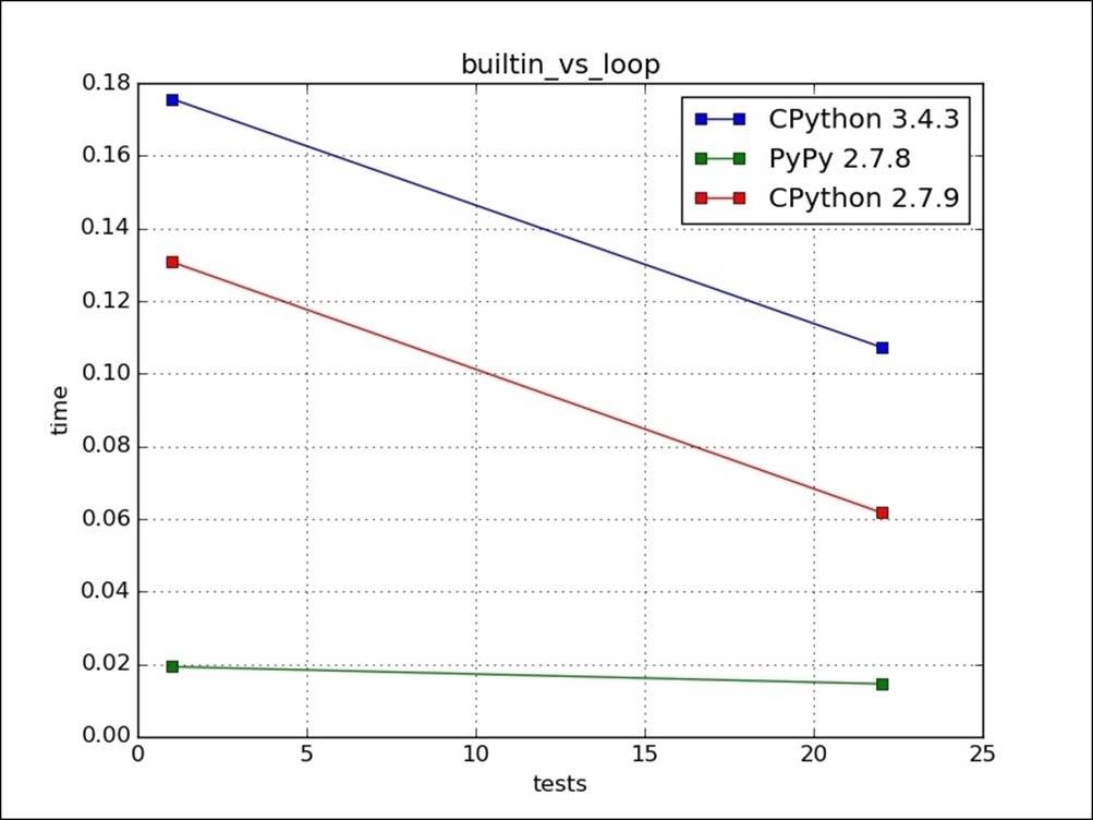
We should pay close attention to not use loops inside loops, giving us quadratic behavior. We can use built-ins, such as map, ZIP, and reduce, instead of using loops if possible. For example, in the following code, the one with map is faster because the looping is implicit and done at C level. By plotting their run times respectively on graph as test 1 and test 2, we see that it is nearly constant for PyPy but reduces a lot for CPython, as follows:
def sqrt_1(ll):
"""simple for loop"""
res = []
for i in ll:
res.append(math.sqrt(i))
return res
def sqrt_2(ll):
"builtin map"
return list(map(math.sqrt,ll))
The test 1 is for sqrt_1(list(range(1000))) and test 22 sqrt_2(list(range(1000))).
The following image is a graphical representation of the preceding code:
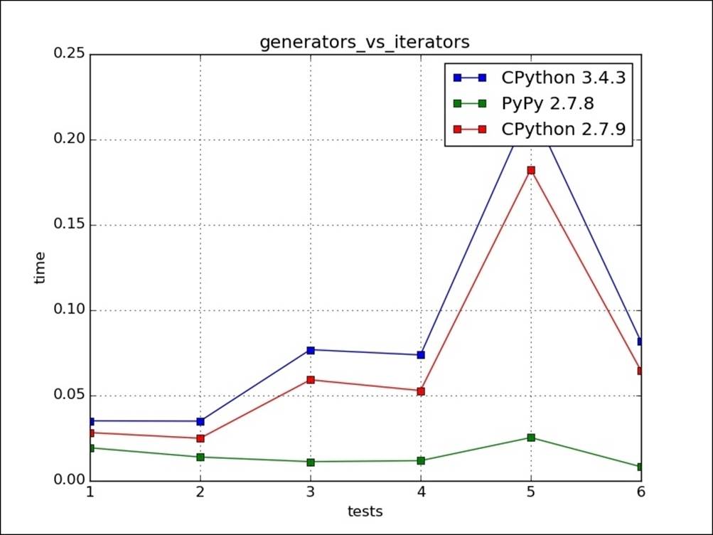
Generators should be used, when the result that is consumed is averagely smaller than the total result consumed. In other words, the result that is generated in the end may not be used. They also serve to conserve memory because no temporary result is stored but generated on demand. In the following example, sqrt_5 creates a generator, while sqrt_6 creates a list. The use_combo instance breaks out of the loop of iteration after a given number of iterations. Test 1 runs use_combo(sqrt_5,range(10),5) and all results are consumed from iterator, whereas test 2 is for the use_combo(sqrt_6,range(10),5) generator. Test 1 should take more time than test 2 as it creates results for all ranges of inputs. Tests 3, and 4 are run with a range of 25, and tests 5, and 6 are run with a range of 100. As it can be seen, the time consumption variation increases with no of elements in the list:
def sqrt_5(ll):
"simple for loop, yield"
for i in ll:
yield i,math.sqrt(i)
def sqrt_6(ll):
"simple for loop"
res = []
for i in ll:
res.append((i,math.sqrt(i)))
return res
def use_combo(combofunc,ll,no):
for i,j in combofunc(ll):
if i>no:
return j
The following image is the graphical representation of the preceding code:
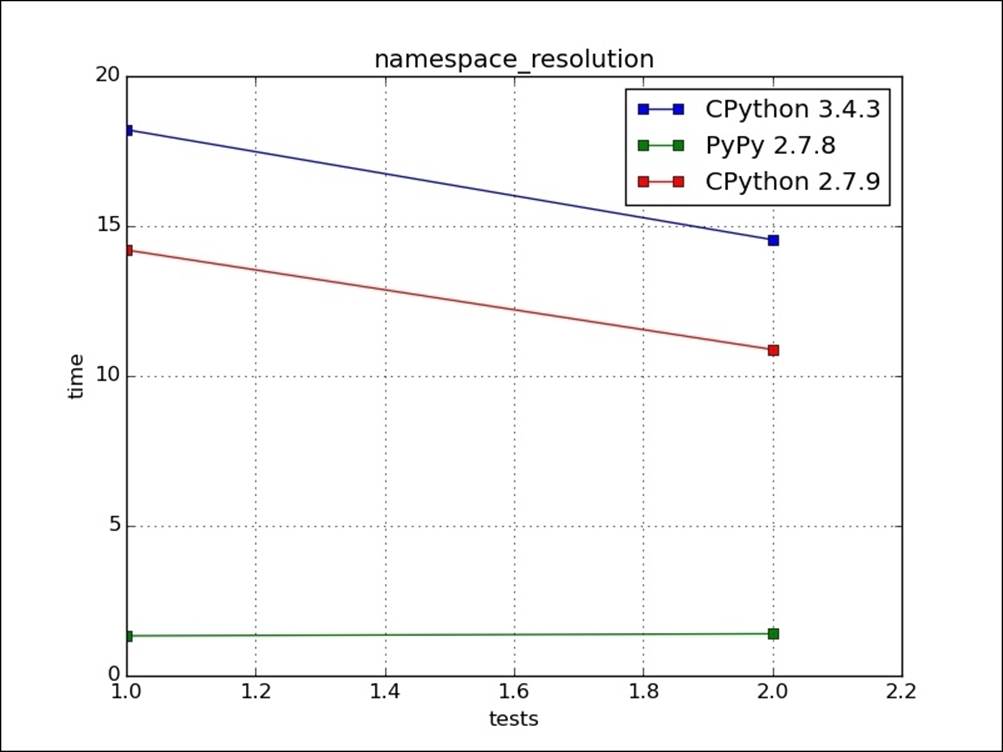
When we are inside a loop and reference an outside namespace variable, it is first searched in local, then nonlocal, followed by global, and then built-in scopes. If the number of repetitions are more, then such overheads add up. We can reduce namespace lookup by making such global/built-in objects available in the local namespace. For example, in the following code snippet, sqrt_7(test2) will be faster than sqrt_1(test1) because of the same reasons:
def sqrt_1(ll):
"""simple for loop"""
res = []
for i in ll:
res.append(math.sqrt(i))
return res
def sqrt_7(ll):
"simple for loop,local"
sqrt = math.sqrt
res = []
for i in ll:
res.append(sqrt(i))
return res
The following image is the graphical representation of the preceding code:
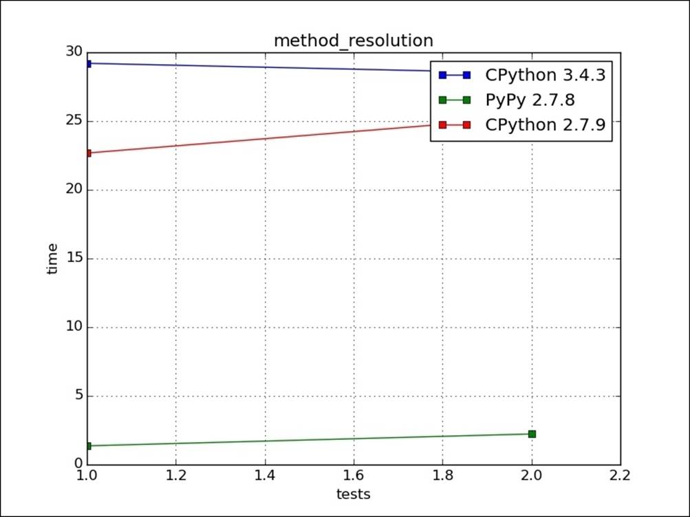
The cost of subclassing is not much and subclassing doesn't make method calls slower even if common sense says that it will take lot of time to look a method up on the inheritance hierarchy. Let's take the following example:
class Super1(object):
def get_sqrt(self,no):
return math.sqrt(no)
class Super2(Super1):
pass
class Super3(Super2):
pass
class Super4(Super3):
pass
class Super5(Super4):
pass
class Super6(Super5):
pass
class Super7(Super6):
pass
class Actual(Super7):
"""method resolution via hierarchy"""
pass
class Actual2(object):
"""method resolution single step"""
def get_sqrt(self,no):
return math.sqrt(no)
def use_sqrt_class(aclass,ll):
cls_instance = aclass()
res = []
for i in ll:
res.append(cls_instance.get_sqrt(i))
return res
Here, if we call get_sqrt on the Actual(case1) class, we need to search it seven levels deep in its base classes, whereas for the Actual2(case2) class it is present on the class itself. The following graph is our plot for both scenarios:
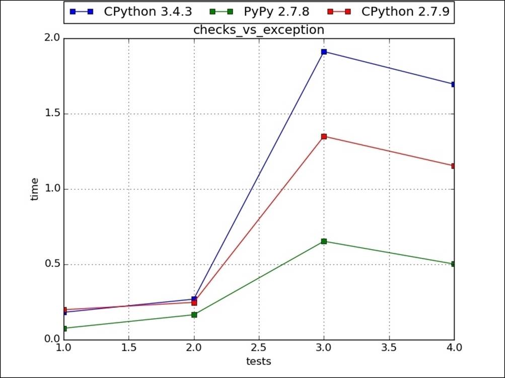
Also, if we are using too many checks in the program logic for return codes or error conditions, we should see how many such checks are really needed. We can write the program logic without using any checks and then get the errors in the exception handling logic. This makes the code easy to understand. As in the following example, the getf_1 function uses checks to filter out error conditions, but too many checks are making code hard to understand. The other get_f2 function is the same application logic or algorithm with exception handling. For test 1 (get_f1) and test 2 (get_f2), no file is present, so all exceptions are raised. In this scenario, the exception handling logic, that is test 2, takes more time. For test 3 (get_f1) and test 4 (get_f2), the file and key are present; hence, no error is raised. In this case, test 4 takes less time, as follows:
def getf_1(ll):
"simple for loop,checks"
res = []
for fname in ll:
curr = []
if os.path.exists(fname):
f = open(fname,"r")
try:
fdict = json.load(f)
except (TypeError, ValueError):
curr = [fname,None,"Unable to read Json"]
finally:
f.close()
if 'name' in fdict:
curr = [fname,fdict["name"],'']
else:
curr = [fname,None,"Key not found in file"]
else:
curr = [fname,None,"file not found"]
res.append(curr)
return res
def getf_2(ll):
"simple for loop, try-except"
res = []
for fname in ll:
try:
f = open(fname,"r")
res.append([fname,json.load(f)['name'],''])
except IOError:
res.append([fname,None,"File Not Found Error"])
except TypeError:
res.append([fname,None,'Unable to read Json'])
except KeyError:
res.append([fname,None,'Key not found in file'])
except Exception as e:
res.append([fname,None,str(e)])
finally:
if 'f' in locals():
f.close()
return res
The following image is the graphical representation of the preceding code:
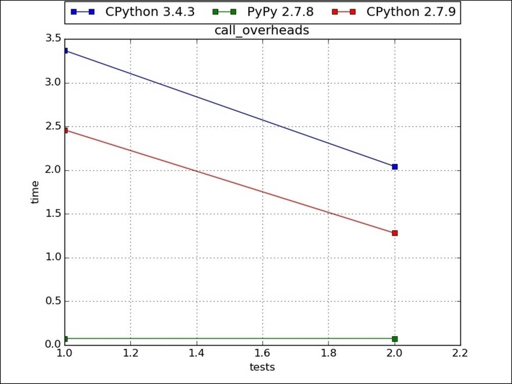
Function calling has overheads and if the performance bottlenecks can be removed by reducing function calls, we should do so. Typically, functions call in loops. In the following example, when we wrote logic inline, it took less time. Also, for PyPy such effects are less in general as most called functions in loops are generally called with the same type of arguments; hence, they get compiled. Any further call to these functions is like calling a C language function:
def please_sqrt(no):
return math.sqrt(no)
def get_sqrt(no):
return please_sqrt(no)
def use_sqrt1(ll,no):
for i in ll:
res = get_sqrt(i)
if res >= no:
return i
def use_sqrt2(ll,no):
for i in ll:
res = math.sqrt(i)
if res >= no:
return i
The following image is the graphical representation of the preceding code:
Profiling to find bottlenecks
Key 2: Identifying application performance bottlenecks.
We should not rely on our intuition on how to optimize application. There are two major ways for logic slowdown; one is CPU time taken, and the second is the wait for results from some other entity. By profiling, we can find out such cases in which we can tweak logic, and language syntax to get better performance on the same hardware. The following code is a showtime decorator that I use to calculate the time taken to call a function. It is simple and effective to get rapid answers:
from datetime import datetime,timedelta
from functools import wraps
import time
def showtime(func):
@wraps(func)
def wrap(*args,**kwargs):
st = time.time() #time clock can be used too
result = func(*args,**kwargs)
et = time.time()
print("%s:%s"%(func.__name__,et-st))
return result
return wrap
@showtime
def func_c():
for i in range(1000):
for j in range(1000):
for k in range(100):
pass
if __name__ == '__main__':
func_c()
This will give us the following output:
(py35) [ ch7 ] $ python code_1_8.py
func_c:1.3181400299072266
When profiling a single large function that does a lot of stuff, we may need to know on what particular line we are spending the most time. This query can be answered using the line_profiler module. You can get it with pip install line_profiler. It shows the time that is spent per line. To get results, we should decorate the function with a special profile decorator that will be used by line_profiler:
from datetime import datetime,timedelta
from functools import wraps
import time
import line_profiler
l = []
def func_a():
global l
for i in range(10000):
l.append(i)
def func_b():
m = list(range(100000))
def func_c():
func_a()
func_b()
k = list(range(100000))
if __name__ == '__main__':
profiler = line_profiler.LineProfiler()
profiler.add_function(func_c)
profiler.run('func_c()')
profiler.print_stats()
This will give us the following output:
Timer unit: 1e-06 s
Total time: 0.007759 s
File: code_1_9.py
Function: func_c at line 15
Line # Hits Time Per Hit % Time Line Contents
==============================================================
15 def func_c():
16 1 2976 2976.0 38.4 func_a()
17 1 2824 2824.0 36.4 func_b()
18 1 1959 1959.0 25.2 k = list(range(100000))
Another way of profiling is using the kernprof program that is supplied with the line_profiler module. We have to decorate the function to be a profiler by the @profile decorator and run the program, as shown in the following code snippet:
from datetime import datetime,timedelta
from functools import wraps
import time
l = []
def func_a():
global l
for i in range(10000):
l.append(i)
def func_b():
m = list(range(100000))
@profile
def func_c():
func_a()
func_b()
k = list(range(100000))
The output for this will be as follows:
(py35) [ ch7 ] $ kernprof -l -v code_1_10.py
Wrote profile results to code_1_10.py.lprof
Timer unit: 1e-06 s
Total time: 0 s
File: code_1_10.py
Function: func_c at line 14
Line # Hits Time Per Hit % Time Line Contents
==============================================================
14 @profile
15 def func_c():
16 func_a()
17 func_b()
18 k = list(range(100000))
Memory profilers are a very good tool to estimate memory consumption in a program. To profile a function, simply decorate it with profile and run the program like this:
from memory_profiler import profile
@profile(precision=4)
def sample():
l1 = [ i for i in range(10000)]
l2 = [ i for i in range(1000)]
l3 = [ i for i in range(100000)]
return 0
if __name__ == '__main__':
sample()
To get details on the command line, use the following code:
(py36)[ ch7 ] $ python ex7_1.py
Filename: ex7_1.py
Line # Mem usage Increment Line Contents
================================================
8 12.6 MiB 0.0 MiB @profile
9 def sample():
10 13.1 MiB 0.5 MiB l1 = [ i for i in range(10000)]
11 13.1 MiB 0.0 MiB l2 = [ i for i in range(1000)]
12 17.0 MiB 3.9 MiB l3 = [ i for i in range(100000)]
13 17.0 MiB 0.0 MiB return 0
Filename: ex7_1.py
Line # Mem usage Increment Line Contents
================================================
10 13.1 MiB 0.0 MiB l1 = [ i for i in range(10000)]
Filename: ex7_1.py
Line # Mem usage Increment Line Contents
================================================
12 17.0 MiB 0.0 MiB l3 = [ i for i in range(100000)]
Filename: ex7_1.py
Line # Mem usage Increment Line Contents
================================================
11 13.1 MiB 0.0 MiB l2 = [ i for i in range(1000)]
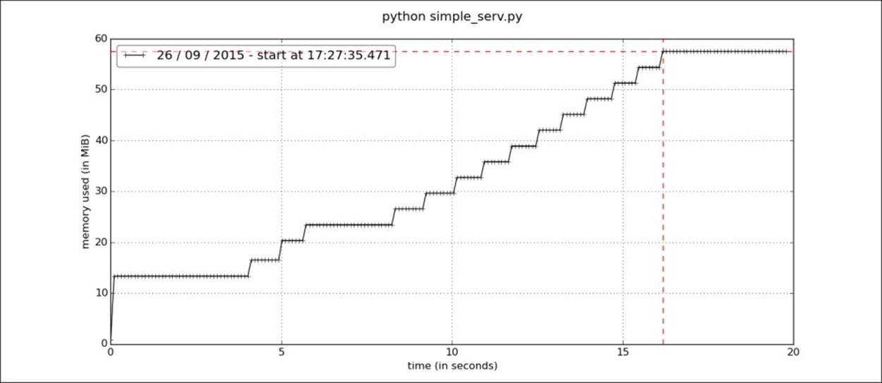
We can also use it to debug long-running programs. The following code is for a simple socket server. It adds lists to the global lists variable, which never gets deleted. Saving contents in simple_serv.py is as follows:
from SocketServer import BaseRequestHandler,TCPServer
lists = []
class Handler(BaseRequestHandler):
def handle(self):
data = self.request.recv(1024).strip()
lists.append(list(range(100000)))
self.request.sendall("server got "+data)
if __name__ == '__main__':
HOST,PORT = "localhost",9999
server = TCPServer((HOST,PORT),Handler)
server.serve_forever()
Now, run the program via profiler as follows:
mprof run simple_serv.py
Put some bogus hits to the server. I used the netcat utility:
[ ch7 ] $ nc localhost 9999 <<END
hello
END
Kill the server after some time and plot the memory consumed over time with the following code:
[ ch7 ] $ mprof plot
We get a good graph showing us memory consumption over time:
Other than getting program memory consumption, we may be interested in objects carrying spaces. Objgraph (https://pypi.python.org/pypi/objgraph) is able to graph object links for your programs. Guppy (https://pypi.python.org/pypi/guppy/) is another package that has heapy, which is a heap analysis tool. It is very helpful to see the number of objects on heap for a running program. As of this writing, it was only available for Python 2. For analysis of a long-running process, Dowser (https://pypi.python.org/pypi/dowser) is also a good choice. We can use Dowser to see the memory consumption to run Celery or a WSGI server. Django-Dowser is good and provides the same functionality as an app, but as the name suggests, it only works with Django.
Using fast libraries
Key 3: Use easy drop-in faster libraries.
There are libraries out there that can help a lot in optimizing code, rather than writing some optimized routines yourself. For example, if we have a list that needs to be fast at FIFO, we may use the blist package. We can use C versions of libraries, such ascStringIO (faster StringIO), ujson (faster JSON handling), numpy (math, and vectors), and lxml (XML handling). Most of the libraries that are listed here are just a Python wrapper over C libraries. You only need to search once for your problem domain. Other than this, we can make a C, or C++ library interface with Python very easily, which is also our next topic.
Using C speeds
Key 4: Running at C speeds.
SWIG
SWIG is an interface compiler that connects programs written in C, and C++ with scripting languages. We can use SWIG to call C, C++ compiled in Python. Let's say that we have a factorial computing library in C, with source code in the fact.c file and the corresponding fact.h header file:
The source code in fact.c is as follows:
#include "fact.h"
long int fact(long int n) {
if (n < 0){
return 0;
}
if (n == 0) {
return 1;
}
else {
return n * fact(n-1);
}
}
The source code in fact.h is as follows:
long int fact(long int n);
Now, we need to write an interface file for SWIG, which tells it what it needs to be exposed to Python:
/* File: fact.i */
%module fact
%{
#define SWIG_FILE_WITH_INIT
#include "fact.h"
%}
long int fact(long int n);
Here, module indicates the module name for the Python library, and SWIG_FILE_WITH_INIT indicates that the resulting C code should be built with a Python extension. The content in {% %} is used in the C wrap code that is generated. We have three files, fact.c, fact.h, and fact.i, in directory. We run SWIG to generate wrapper_code as follows:
swig3.0 -python -O -py3 fact.i
The -O option is used for optimizations and -py3 is for Python 3 specific features.
This generates fact.py and fact_wrap.c. The fact.py is a Python module and fact_wrap.c is the glue code between C and Python:
gcc -fpic -c fact_wrap.c fact.c -I/home/arun/.virtualenvs/py3/include/python3.4m
Here, I have to include my python.h path to compile it. This will generate fact.o and fact_wrap.o. Now, the last part is to create a dynamic linked library, as follows:
gcc -shared fact.o fact_wrap.o -o _fact.so
The _fact.so file is used by the fact.py to run C functions. Now, we can use the fact module in our Python programs:
>>> from fact import fact
>>> fact(10)
3628800
>>> fact(5)
120
>>> fact(20)
2432902008176640000
CFFI
The C Foreign Function Interface (CFFI) for Python is one tool that looks the best to me because of the easy setup and interface. It works on an ABI and API level.
Using our factorial C programs here as well, we first create a shared library for the code:
gcc -shared fact.o -o _fact.so
gcc -fpic -c fact.c -o fact.o
Now, we have a _fact.so shared library object in our current directory. To load this in the Python environment, we can perform this action which is very straightforward. We should have header files for the library so that we can use declarations. Install the CFFI package from distribution or pip that is needed for this, as follows:
>>> from cffi import FFI
>>> ffi = FFI()
>>> ffi.cdef("""
... long int fact(long int num);
... """)
>>> C = ffi.dlopen("./_fact.so")
>>> C.fact(20)
2432902008176640000
We can reduce import times for the module if we do not call cdef in the import modules. We can write another setup_fact_ffi.py module that gives us a fact_ffi.py module with the compiled information. Hence, the load times decrease a lot:
from cffi import FFI
ffi = FFI()
ffi.set_source("fact_ffi", None)
ffi.cdef("""
long int fact(long int n);
""")
if __name__ == "__main__":
ffi.compile()
python setup_fact_ffi.py
We now can use this module to get ffi and load our shared library as follows:
>>> from fact_ffi import ffi
>>> ll = ffi.dlopen("./_fact.so")
>>> ll.fact(20)
2432902008176640000
>>>
Until this point, as we were using a precompiled shared library, we didn't need a compiler. Let's suppose that there is this small C function that you need in Python, and you do not want to write another .c file for it, then this is how it can be done. You can also extend it to shared libraries as well.
First, we define a build_ffi.py file, which will compile and create a module for us:
__author__ = 'arun'
from cffi import FFI
ffi = FFI()
ffi.set_source("_fact_cffi",
"""
long int fact(long int n) {
if (n < 0){
return 0;
}
if (n == 0) {
return 1;
}
else {
return n * fact(n-1);
}
}
""",
libraries=[]
)
ffi.cdef("""
long int fact(long int n);
""")
if __name__ == '__main__':
ffi.compile()
When we run Python fact_build.py, this will create a _fact_cffi.cpython-34m.so module. To use it, we have to import it and use the lib variable to access the module:
>>> from _fact_cffi import ffi,lib
>>> lib.fact(20)
Cython
Cython is like a superset of Python in which we can optionally give static declarations. The source code is compiled to C/C++ extension modules.
We write our old factorial program in fact_cpy.pyx as follows:
cpdef double fact(int num):
cdef double res = 1
if num < 0:
return -1
elif num == 0:
return 1
else:
for i in range(1,num + 1):
res = res*i
return res
Here cpdef is the function declaration for CPython that creates a Python function and conversion logic for arguments, and a C function that actually executes. cpdef is defining the data type for the res variable, which helps in speedup.
We have to create a setup.py file to compile this code into an extension module (we can directly use it by using pyximport but we will leave that for now). The contents for the setup.py file will be as follows:
from distutils.core import setup
from Cython.Build import cythonize
setup(
name = 'factorial library',
ext_modules = cythonize("fact_cpy.pyx"),
)
Now to build the module, all we have to do is type in the following command, and we get a fact_cpy.cpython-34m.so file in the current directory:
python setup.py build_ext --inplace
Using this in Python is as follows:
>>> from fact_cpy import fact
>>> fact(20)
2432902008176640000
Summary
In this chapter, we saw various techniques that are used to optimize and profile code. I will, again, point out that we should always focus on first writing the correct program, then writing test cases for it, and then optimizing it. We should write code with optimizations that we know at that time or without optimization the first time, and we should hunt for them only if we need them from a business perspective. Compiling a C module can give a good speedup for CPU-intensive tasks. Also, we can give up GIL in C modules, which can also help us in increasing performance. But, all of this was on single system. Now, in the next chapter, we will see how we can improve performance when the tricks that were discussed in this chapter are not sufficient for a real-life scenario.
All materials on the site are licensed Creative Commons Attribution-Sharealike 3.0 Unported CC BY-SA 3.0 & GNU Free Documentation License (GFDL)
If you are the copyright holder of any material contained on our site and intend to remove it, please contact our site administrator for approval.
© 2016-2026 All site design rights belong to S.Y.A.