Algorithms (2014)
Three. Searching
3.4 Hash Tables
If keys are small integers, we can use an array to implement an unordered symbol table, by interpreting the key as an array index so that we can store the value associated with key i in array entry i, ready for immediate access. In this section, we consider hashing, an extension of this simple method that handles more complicated types of keys. We reference key-value pairs using arrays by doing arithmetic operations to transform keys into array indices.
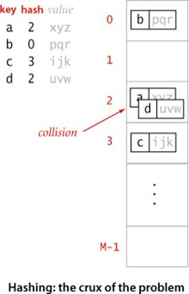
Search algorithms that use hashing consist of two separate parts. The first part is to compute a hash function that transforms the search key into an array index. Ideally, different keys would map to different indices. This ideal is generally beyond our reach, so we have to face the possibility that two or more different keys may hash to the same array index. Thus, the second part of a hashing search is a collision-resolution process that deals with this situation. After describing ways to compute hash functions, we shall consider two different approaches to collision resolution: separate chaining and linear probing.
Hashing is a classic example of a time-space tradeoff. If there were no memory limitation, then we could do any search with only one memory access by simply using the key as an index in a (potentially huge) array. This ideal often cannot be achieved, however, because the amount of memory required is prohibitive when the number of possible key values is huge. On the other hand, if there were no time limitation, then we can get by with only a minimum amount of memory by using sequential search in an unordered array. Hashing provides a way to use a reasonable amount of both memory and time to strike a balance between these two extremes. Indeed, it turns out that we can trade off time and memory in hashing algorithms by adjusting parameters, not by rewriting code. To help choose values of the parameters, we use classical results from probability theory.
Probability theory is a triumph of mathematical analysis that is beyond the scope of this book, but the hashing algorithms we consider that take advantage of the knowledge gained from that theory are quite simple, and widely used. With hashing, you can implement search and insert for symbol tables that require constant (amortized) time per operation in typical applications, making it the method of choice for implementing basic symbol tables in many situations.
Hash functions
The first problem that we face is the computation of the hash function, which transforms keys into array indices. If we have an array that can hold M key-value pairs, then we need a hash function that can transform any given key into an index into that array: an integer in the range [0, M − 1]. We seek a hash function that both is easy to compute and uniformly distributes the keys: for each key, every integer between 0 and M − 1 should be equally likely (independently for every key). This ideal is somewhat mysterious; to understand hashing, we to begin by thinking carefully about how to implement such a function.
In principle, any key can be represented as a sequence of bits, so we might design a generic hash function that maps sequences of bits to integers in the desired range. In practice, programmers implement hash functions based on higher-level representations. For example, if the key involves a number, such as a social security number, we could start with that number; if the key involves a string, such as a person’s name, we need to convert the string into a number; and if the key has multiple parts, such as a mailing address, we need to combine the parts somehow. For many common types of keys, we can make use of default implementations provided by Java. We briefly discuss potential implementations for various types of keys so that you can see what is involved because you do need to provide implementations for key types that you create.
Typical example
Suppose that we have an application where the keys are U.S. social security numbers. A social security number such as 123-45-6789 is a nine-digit number divided into three fields. The first field identifies the geographical area where the number was issued (for example, social security numbers whose first field is 035 are from Rhode Island and numbers whose first field is 214 are from Maryland) and the other two fields identify the individual. There are a billion (109) different social security numbers, but suppose that our application will need to process just a few hundred keys, so that we could use a hash table of size M = 1,000. One possible approach to implementing a hash function is to use three digits from the key. Using three digits from the third field is likely to be preferable to using the three digits in the first field (since customers may not be uniformly dispersed over geographic areas), but a better approach is to use all nine digits to make an int value, then consider hash functions for integers, described next.
Positive integers
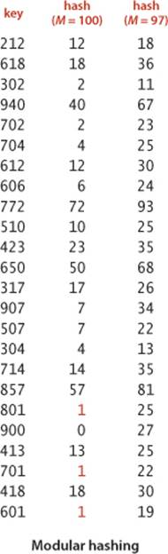
The most commonly used method for hashing integers is called modular hashing: we choose the array size M to be prime and, for any positive integer key k, compute the remainder when dividing k by M. This function is very easy to compute (k % M, in Java) and is effective in dispersing the keys evenly between 0 and M − 1. If M is not prime, it may be the case that not all of the bits of the key play a role, which amounts to missing an opportunity to disperse the values evenly. For example, if the keys are base-10 numbers and M is 10k, then only the k least significant digits are used. As a simple example where such a choice might be problematic, suppose that the keys are telephone area codes and M = 100. For historical reasons, most area codes in the United States have middle digit 0 or 1, so this choice strongly favors the values less than 20, where the use of the prime value 97 better disperses them (a prime value not close to 100 would do even better). Similarly, IP addresses that are used in the internet are binary numbers that are not random for similar historical reasons as for telephone area codes, so we need to use a table size that is a prime (in particular, not a power of 2) if we want to use modular hashing to disperse them.
Floating-point numbers
If the keys are real numbers between 0 and 1, we might just multiply by M and round off to the nearest integer to get an index between 0 and M − 1. Although this approach is intuitive, it is defective because it gives more weight to the most significant bits of the keys; the least significant bits play no role. One way to address this situation is to use modular hashing on the binary representation of the key (this is what Java does).
Strings
Modular hashing works for long keys such as strings, too: we simply treat them as huge integers. For example, the code at left computes a modular hash function for a String s: recall that charAt() returns a char value in Java, which is a 16-bit nonnegative integer. If R is greater than any character value, this computation would be equivalent to treating the String as an N-digit base-R integer, computing the remainder that results when dividing that number by M. A classic algorithm known as Horner’s method gets the job done with N multiplications, additions, and remainder operations. If the value of R is sufficiently small that no overflow occurs, the result is an integer between 0 and M − 1, as desired. The use of a small prime integer such as 31 ensures that the bits of all the characters play a role. Java’s default implementation for String uses a method like this.
Hashing a string key
int hash = 0;
for (int i = 0; i < s.length(); i++)
hash = (R * hash + s.charAt(i)) % M;
Compound keys
If the key type has multiple integer fields, we can typically mix them together in the way just described for String values. For example, suppose that search keys are of type Date, which has three integer fields: day (two-digit day), month (two-digit month), and year (four-digit year). We compute the number
int hash = (((day * R + month) % M ) * R + year) % M;
which, if the value of R is sufficiently small that no overflow occurs, is an integer between 0 and M − 1, as desired. In this case, we could save the cost of the inner % M operation by choosing a moderate prime value such as 31 for R. As with strings, this method generalizes to handle any number of fields.
Java conventions
Java helps us address the basic problem that every type of data needs a hash function by ensuring that every data type inherits a method called hashCode() that returns a 32-bit integer. The implementation of hashCode() for a data type must be consistent with equals. That is, if a.equals(b) is true, thena.hashCode() must have the same numerical value as b.hashCode(). Conversely, if the hashCode() values are different, then we know that the objects are not equal. If the hashCode() values are the same, the objects may or may not be equal, and we must use equals() to decide which condition holds. This convention is a basic requirement for clients to be able to use hashCode() for symbol tables. Note that it implies that you must override both hashCode() and equals() if you need to hash with a user-defined type. The default implementation returns the machine address of the key object, which is seldom what you want. Java provides hashCode() implementations that override the defaults for many common types (including String, Integer, Double, File, and URL).
Converting a hashCode() to an array index
Since our goal is an array index, not a 32-bit integer, we combine hashCode() with modular hashing in our implementations to produce integers between 0 and M − 1, as follows:
private int hash(Key x)
{ return (x.hashCode() & 0x7fffffff) % M; }
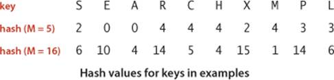
This code masks off the sign bit (to turn the 32-bit number into a 31-bit nonnegative integer) and then computes the remainder when dividing by M, as in modular hashing. Programmers commonly use a prime number for the hash table size M when using code like this, to attempt to make use of all the bits of the hash code. Note: To avoid confusion, we omit all of these calculations in our hashing examples and use instead the hash values in the table at right.
User-defined hashCode()
Client code expects that hashCode() disperses the keys uniformly among the possible 32-bit result values. That is, for any object x, you can write x.hashCode() and, in principle, expect to get any one of the 232 possible 32-bit values with equal likelihood. Java’s hashCode() implementations for String,Integer, Double, File, and URL aspire to this functionality; for your own type, you have to try to do it on your own. The Date example that we considered on page 460 illustrates one way to proceed: make integers from the instance variables and use modular hashing. In Java, the convention that all data types inherit a hashCode() method enables an even simpler approach: use the hashCode() method for the instance variables to convert each to a 32-bit int value and then do the arithmetic, as illustrated at left for Transaction. For primitive-type instance variables, note that a cast to a wrapper type is necessary to access the hashCode() method. Again, the precise values of the multiplier (31 in our example) is not particularly important.
Implementing hashCode() in a user-defined type
public class Transaction
{
...
private final String who;
private final Date when;
private final double amount;
public int hashCode()
{
int hash = 17;
hash = 31 * hash + who.hashCode();
hash = 31 * hash + when.hashCode();
hash = 31 * hash
+ ((Double) amount).hashCode();
return hash;
}
...
}
Software caching
If computing the hash code is expensive, it may be worthwhile to cache the hash for each key. That is, we maintain an instance variable hash in the key type that contains the value of hashCode() for each key object (see EXERCISE 3.4.25). On the first call to hashCode(), we have to compute the full hash code (and set the value of hash), but subsequent calls on hashCode() simply return the value of hash. Java uses this technique to reduce the cost of computing hashCode() for String objects.
IN SUMMARY, WE HAVE THREE PRIMARY REQUIREMENTS in implementing a good hash function for a given data type:
• It should be consistent—equal keys must produce the same hash value.
• It should be efficient to compute.
• It should uniformly distribute the set of keys.
Satisfying these requirements simultaneously in Java is a job for experts. As with many built-in capabilities, Java programmers who use hashing assume that hashCode() does the job, absent any evidence to the contrary.
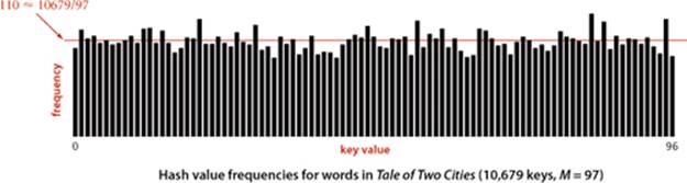
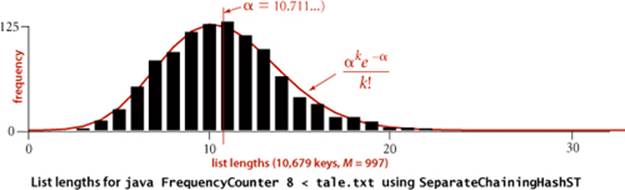
Still, you should be vigilant whenever using hashing in situations where good performance is critical, because a bad hash function is a classic example of a performance bug: everything will work properly, but much more slowly than expected. Perhaps the easiest way to ensure uniformity is to make sure that all the bits of the key play an equal role in computing every hash value; perhaps the most common mistake in implementing hash functions is to ignore significant numbers of the key bits. Whatever the implementation, it is wise to test any hash function that you use, when performance is important. Which takes more time: computing a hash function or comparing two keys? Does your hash function spread a typical set of keys uniformly among the values between 0 and M − 1? Doing simple experiments that answer these questions can protect future clients from unfortunate surprises. For example, the histogram above shows that our hash() implementation using the hashCode() from Java’s String data type produces a reasonable dispersion of the words for our Tale of Two Cities example.
Underlying this discussion is a fundamental assumption that we make when using hashing; it is an idealized model that we do not actually expect to achieve, but it guides our thinking when implementing hashing algorithms and facilitates their analyses:
Assumption J (uniform hashing assumption). The hash functions that we use uniformly and independently distribute keys among the integer values between 0 and M − 1.
Discussion: With all of the arbitrary choices we have made, the Java hash functions that we have considered do not satisfy these conditions; nor can any deterministic hash function. The idea of constructing hash functions that uniformly and independently distribute keys leads to deep issues in theoretical computer science. In 1977, L. Carter and M. Wegman described how to construct auniversal family of hash functions. If a hash function is chosen at random from a universal family, the hash function uniformly distributes the keys, but only with partial independence. Although weaker than full independence, the partial independence is sufficient to establish performance guarantees similar to those stated in Propositions K and M.
ASSUMPTION J is a useful way to think about hashing for two primary reasons. First, it is a worthy goal when designing hash functions that guides us away from making arbitrary decisions that might lead to an excessive number of collisions. Second, we will use it to develop hypotheses about the performance of hashing —even when hash functions are not known to satisfy ASSUMPTION J, we can perform computational experiments and validate that they achieve the predicted performance.
Hashing with separate chaining
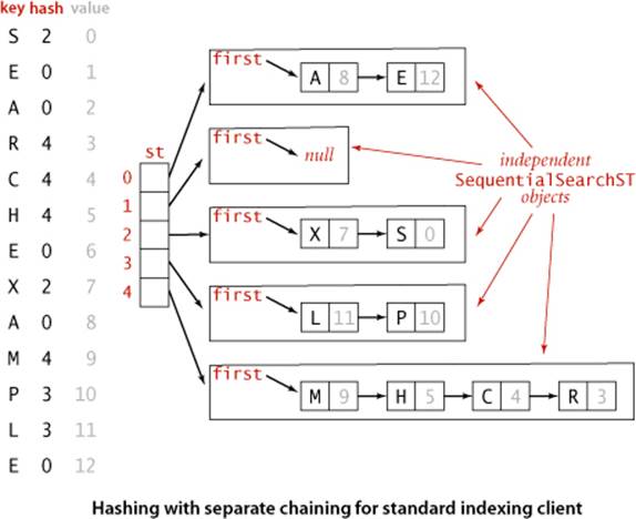
A hash function converts keys into array indices. The second component of a hashing algorithm is collision resolution: a strategy for handling the case when two or more keys to be inserted hash to the same index. A straightforward and general approach to collision resolution is to build, for each of the M array indices, a linked list of the key-value pairs whose keys hash to that index. This method is known as separate chaining because items that collide are chained together in separate linked lists. The basic idea is to choose M to be sufficiently large that the lists are sufficiently short to enable efficient search through a two-step process: hash to find the list that could contain the key, then sequentially search through that list for the key.
One way to proceed is to expand SequentialSearchST (ALGORITHM 3.1) to implement separate chaining using linked-list primitives (see EXERCISE 3.4.2). A simpler (though slightly less efficient) way to proceed is to adopt a more general approach: we build, for each of the M array indices, a symbol table of the keys that hash to that index, thus reusing code that we have already developed. The implementation SeparateChainingHashST in ALGORITHM 3.5 maintains an array of SequentialSearchST objects and implements get() and put() by computing a hash function to choose which SequentialSearchSTobject can contain the key and then using get() and put() (respectively) from SequentialSearchST to complete the job.
Since we have M lists and N keys, the average length of the lists is always N / M, no matter how the keys are distributed among the lists. For example, suppose that all the items fall onto the first list—the average length of the lists is (N + 0 + 0 + 0 + . . . + 0)/M = N / M. However the keys are distributed on the lists, the sum of the list lengths is N and the average is N / M. Separate chaining is useful in practice because each list is extremely likely to have about N / M key-value pairs. In typical situations, we can verify this consequence of ASSUMPTION J and count on fast search and insert.
Algorithm 3.5 Hashing with separate chaining
public class SeparateChainingHashST<Key, Value>
{
private int M; // hash table size
private SequentialSearchST<Key, Value>[] st; // array of ST objects
public SeparateChainingHashST()
{ this(997); }
public SeparateChainingHashST(int M)
{ // Create M linked lists.
this.M = M;
st = (SequentialSearchST<Key, Value>[]) new SequentialSearchST[M];
for (int i = 0; i < M; i++)
st[i] = new SequentialSearchST();
}
private int hash(Key key)
{ return (key.hashCode() & 0x7fffffff) % M; }
public Value get(Key key)
{ return (Value) st[hash(key)].get(key); }
public void put(Key key, Value val)
{ st[hash(key)].put(key, val); }
public Iterable<Key> keys()
// See Exercise 3.4.19.
}
This basic symbol-table implementation maintains an array of linked lists, using a hash function to choose a list for each key. For simplicity, we use SequentialSearchST methods. We need a cast when creating st[] because Java prohibits arrays with generics. The default constructor specifies 997 lists, so that for large tables, this code is about a factor of 1,000 faster thanSequentialSearchST. This quick solution is an easy way to get good performance when you have some idea of the number of key-value pairs to be put() by a client. A more robust solution is to use array resizing to make sure that the lists are short no matter how many key-value pairs are in the table (see page 474 and EXERCISE 3.4.18).
Proposition K. In a separate-chaining hash table with M lists and N keys, the probability (under ASSUMPTION J) that the number of keys in a list is within a small constant factor of N/M is extremely close to 1.
Proof sketch: ASSUMPTION J makes this an application of classical probability theory. We sketch the proof, for readers who are familiar with basic probabilistic analysis. The probability that a given list will contain exactly k keys is given by the binomial distribution
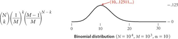
by the following argument: Choose k out of the N keys. Those k keys hash to the given list with probability 1 / M, and the other N − k keys do not hash to the given list with probability 1 − (1 / M). In terms of α = N / M, we can rewrite this expression as
![]()
which (for small α) is closely approximated by the classical Poisson distribution
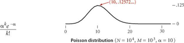
It follows that the probability that a list has more than t α keys on it is bounded by the quantity (α e/t)t e−α. This probability is extremely small for practical ranges of the parameters. For example, if the average length of the lists is 10, the probability that we will hash to some list with more than 20 keys on it is less than (10 e/2)2e−10 ≈ 0.0084, and if the average length of the lists is 20, the probability that we will hash to some list with more than 40 keys on it is less than (20 e/2)2e−20 ≈ 0.0000016. This concentration result does not guarantee that every list will be short. Indeed it is known that, if α is a constant, the average length of the longest list grows with log N/log log N.
This classical mathematical analysis is compelling, but it is important to note that it completely depends on ASSUMPTION J. If the hash function is not uniform and independent, the search and insert cost could be proportional to N, no better than with sequential search. ASSUMPTION J is much stronger than the corresponding assumption for other probabilistic algorithms that we have seen, and much more difficult to verify. With hashing, we are assuming that each and every key, no matter how complex, is equally likely to be hashed to one of M indices. We cannot afford to run experiments to test every possible key, so we would have to do more sophisticated experiments involving random sampling from the set of possible keys used in an application, followed by statistical analysis. Better still, we can use the algorithm itself as part of the test, to validate bothASSUMPTION J and the mathematical results that we derive from it.
Property L. In a separate-chaining hash table with M lists and N keys, the number of compares (equality tests) for search miss and insert is ~N/M.
Evidence: Countless programmers since the 1950s have seen the speedups for separate-chaining hash tables predicted by Proposition K, even for hash functions that clearly do not satisfy Assumption J. For example, the diagram on page 468 shows that list length distribution for our FrequencyCounter example (using our FrequencyCounter example (using our hash() implementation based on the hashCode() from Java’s String data type) precisely matches the theoretical model. One exception that has been documented on numerous occasions is poor performance due to hash functions not taking all of the bits of the keys into account. Otherwise, the preponderance of the evidence from the experience of practical programmers puts us on solid ground in stating that hashing with separate chaining using an array of size M speeds up search and insert in a symbol table by a factor of M.
Table size
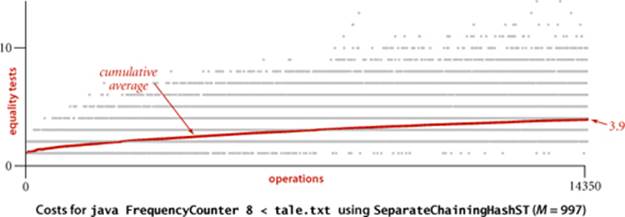
In a separate-chaining implementation, our goal is to choose the table size M to be sufficiently small that we do not waste a huge area of contiguous memory with empty chains but sufficiently large that we do not waste time searching through long chains. One of the virtues of separate chaining is that this decision is not critical: if more keys arrive than expected, then searches will take a little longer than if we had chosen a bigger table size ahead of time; if fewer keys are in the table, then we have extra-fast search with some wasted space. When space is not a critical resource, M can be chosen sufficiently large that search time is constant; when space is a critical resource, we still can get a factor of M improvement in performance by choosing M to be as large as we can afford. For our example FrequencyCounter study, we see in the figure below a reduction in the average cost from thousands of compares per operation for SequentialSearchST to a small constant for SeparateChainingHashST, as expected. Another option is to use array resizing to keep the lists short (see EXERCISE 3.4.18).
Deletion
To delete a key-value pair, simply hash to find the SequentialSearchST containing the key, then invoke the delete() method for that table (see EXERCISE 3.1.5). Reusing code in this way is preferable to reimplementing this basic operation on linked lists.
Ordered operations
The whole point of hashing is to uniformly disperse the keys, so any order in the keys is lost when hashing. If you need to quickly find the maximum or minimum key, find keys in a given range, or implement any of the other operations in the ordered symbol-table API on page 366, then hashing is not appropriate, since these operations will all take linear time.
HASHING WITH SEPARATE CHAINING is easy to implement and probably the fastest (and most widely used) symbol-table implementation for applications where key order is not important. When your keys are built-in Java types or your own type with well-tested implementations of hashCode(),ALGORITHM 3.5 provides a quick and easy path to fast search and insert. Next, we consider an alternative scheme for collision resolution that is also effective.
Hashing with linear probing
Another approach to implementing hashing is to store N key-value pairs in a hash table of size M > N, relying on empty entries in the table to help with collision resolution. Such methods are called open-addressing hashing methods.
The simplest open-addressing method is called linear probing: when there is a collision (when we hash to a table index that is already occupied with a key different from the search key), then we just check the next entry in the table (by incrementing the index). Linear probing is characterized by identifying three possible outcomes:
• Key equal to search key: search hit
• Empty position (null key at indexed position): search miss
• Key not equal to search key: try next entry
We hash the key to a table index, check whether the search key matches the key there, and continue (incrementing the index, wrapping back to the beginning of the table if we reach the end) until finding either the search key or an empty table entry. It is customary to refer to the operation of determining whether or not a given table entry holds an item whose key is equal to the search key as a probe. We use the term interchangeably with the term compare that we have been using, even though some probes are tests for null.
Algorithm 3.6 Hashing with linear probing
public class LinearProbingHashST<Key, Value>
{
private int N; // number of key-value pairs in the table
private int M = 16; // size of linear-probing table
private Key[] keys; // the keys
private Value[] vals; // the values
public LinearProbingHashST()
{
keys = (Key[]) new Object[M];
vals = (Value[]) new Object[M];
}
private int hash(Key key)
{ return (key.hashCode() & 0x7fffffff) % M; }
private void resize() // See page 474.
public void put(Key key, Value val)
{
if (N >= M/2) resize(2*M); // double M (see text)
int i;
for (i = hash(key); keys[i] != null; i = (i + 1) % M)
if (keys[i].equals(key)) { vals[i] = val; return; }
keys[i] = key;
vals[i] = val;
N++;
}
public Value get(Key key)
{
for (int i = hash(key); keys[i] != null; i = (i + 1) % M)
if (keys[i].equals(key))
return vals[i];
return null;
}
}
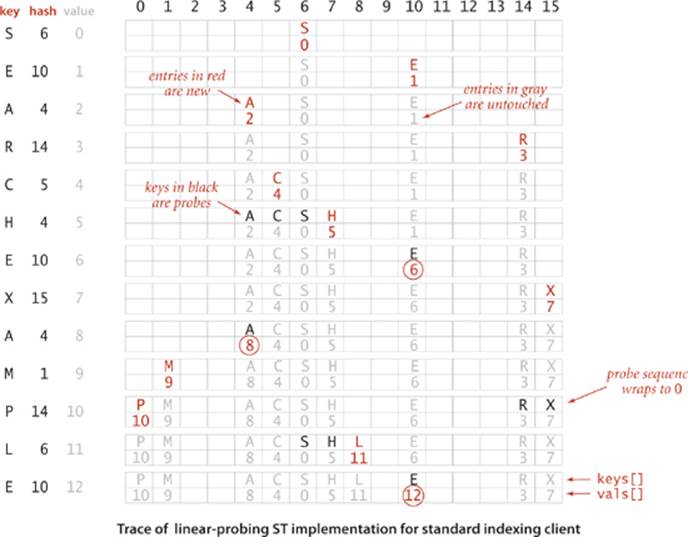
This symbol-table implementation keeps keys and values in parallel arrays (as in BinarySearchST) but uses empty spaces (marked by null) to terminate clusters of keys. If a new key hashes to an empty entry, it is stored there; if not, we scan sequentially to find an empty position. To search for a key, we scan sequentially starting at its hash index until finding null (search miss) or the key (search hit). Implementation of keys() is left as EXERCISE 3.4.19.
The essential idea behind hashing with open addressing is this: rather than using memory space for references in linked lists, we use it for the empty entries in the hash table, which mark the ends of probe sequences. As you can see from LinearProbingHashST (ALGORITHM 3.6), applying this idea to implement the symbol-table API is quite straightforward. We implement the table with parallel arrays, one for the keys and one for the values, and use the hash function as an index to access the data as just discussed.
Deletion
How do we delete a key-value pair from a linear-probing table? If you think about the situation for a moment, you will see that setting the key’s table position to null will not work, because that might prematurely terminate the search for a key that was inserted into the table later. As an example, suppose that we try to delete C in this way in our trace example, then search for H. The hash value for H is 4, but it sits at the end of the cluster, in position 7. If we set position 5 to null, then get() will not find H. As a consequence, we need to reinsert into the table all of the keys in the cluster to the right of the deleted key. This process is trickier than it might seem, so you are encouraged to trace through the code at right (see EXERCISE 3.4.17).
Deletion for linear probing
public void delete(Key key)
{
if (!contains(key)) return;
int i = hash(key);
while (!key.equals(keys[i]))
i = (i + 1) % M;
keys[i] = null;
vals[i] = null;
i = (i + 1) % M;
while (keys[i] != null)
{
Key keyToRedo = keys[i];
Value valToRedo = vals[i];
keys[i] = null;
vals[i] = null;
N--;
put(keyToRedo, valToRedo);
i = (i + 1) % M;
}
N--;
if (N > 0 && N == M/8)
resize(M/2);
}
AS WITH SEPARATE CHAINING, the performance of hashing with open addressing depends on the ratio α = N / M, but we interpret it differently. We refer to α as the load factor of a hash table. For separate chaining, α is the average number of keys per list and is often larger than 1; for linear probing, α is the percentage of table entries that are occupied; it cannot be greater than 1. In fact, we cannot let the load factor reach 1 (completely full table) in LinearProbingHashST because a search miss would go into an infinite loop in a full table. Indeed, for the sake of good performance, we use array resizing to guarantee that the load factor is between one-eighth and one-half. This strategy is validated by mathematical analysis, which we consider before we discuss implementation details.
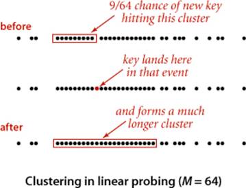
Clustering
The average cost of linear probing depends on the way in which the entries clump together into contiguous groups of occupied table entries, called clusters, when they are inserted. For example, when the key C is inserted in our example, the result is a cluster (A C S) of length 3, which means that four probes are needed to insert H because H hashes to the first position in the cluster. Short clusters are certainly a requirement for efficient performance. This requirement can be problematic as the table fills, because long clusters are common. Moreover, since all table positions are equally likely to be the hash value of the next key to be inserted (under the uniform hashing assumption), long clusters are more likely to increase in length than short ones, because a new key hashing to any entry in the cluster will cause the cluster to increase in length by 1 (and possibly much more, if there is just one table entry separating the cluster from the next one). Next, we turn to the challenge of quantifying the effect of clustering to predict performance in linear probing, and using that knowledge to set design parameters in our implementations.
Analysis of linear probing
Despite the relatively simple form of the results, precise analysis of linear probing is a very challenging task. Knuth’s derivation of the following formulas in 1962 was a landmark in the analysis of algorithms:
Proposition M. In a linear-probing hash table of size M lists and N = α M keys, the average number of probes (under ASSUMPTION J) required is
![]()
for search hits and search misses (or inserts), respectively. In particular, when α is about 1/2, the average number of probes for a search hit is about 3/2 and for a search miss is about 5/2. These estimates lose a bit of precision as α approaches 1, but we do not need them for that case, because we will only use linear probing for α less than one-half.
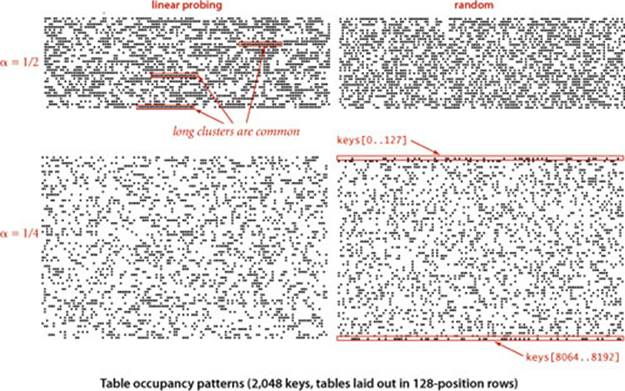
Discussion: We compute the average by computing the cost of a search miss starting at each position in the table, then dividing the total by M. All search misses take at least 1 probe, so we count the number of probes after the first. Consider the following two extremes in a linear-probing table that is half full (M = 2N): In the best case, table positions with even indices could be empty, and table positions with odd indices could be occupied. In the worst case, the first half of the table positions could be empty, and the second half occupied. The average length of the clusters in both cases is N/(2N) = 1/2, but the average number of probes for a search miss is 1 (all searches take at least 1 probe) plus (0 + 1 + 0 + 1 + . . .)/(2N) = 1/2 in the best case, and is 1 plus (N + (N − 1) + . . .) / (2N) ~ N/4 in the worst case. This argument generalizes to show that the average number of probes for a search miss is proportional to the squares of the lengths of the clusters: If a cluster is of length t, then the expression (t + (t − 1) + . . . + 2 + 1) / M = t(t + 1)/(2M) counts the contribution of that cluster to the grand total. The sum of the cluster lengths is N, so, adding this cost for all entries in the table, we find that the total average cost for a search miss is 1 + N / (2M) plus the sum of the squares of the lengths of the clusters, divided by 2M. Thus, given a table, we can quickly compute the average cost of a search miss in that table (see EXERCISE 3.4.21). In general, the clusters are formed by a complicated dynamic process (the linear-probing algorithm) that is difficult to characterize analytically, and quite beyond the scope of this book.
PROPOSITION M tells us (under our usual ASSUMPTION J) that we can expect a search to require a huge number of probes in a nearly full table (as α approaches 1 the values of the formulas describing the number of probes grow very large) but that the expected number of probes is between 1.5 and 2.5 if we can ensure that the load factor α is less than 1/2. Next, we consider the use of array resizing for this purpose.
Array resizing
We can use our standard array-resizing technique from CHAPTER 1 to ensure that the load factor never exceeds one-half. First, we need a new constructor for LinearProbingHashST that takes a fixed capacity as argument (add a line to the constructor in ALGORITHM 3.6 that sets M to the given value before creating the arrays). Next, we need the resize() method given at left, which creates a new LinearProbingHashST of the given size and, puts all the key-value pairs from the old table into the new one by rehashing all the keys These additions allow us to implement array doubling. The call toresize() in the first statement in put() ensures that the table is at most one-half full. This code builds a hash table twice the size with the same keys, thus halving the value of α. As in other applications of array resizing, we also need to add
if (N > 0 && N <= M/8) resize(M/2);
Resizing a linear-probing hash table
private void resize(int cap)
{
LinearProbingHashST<Key, Value> t;
t = new LinearProbingHashST<Key, Value>(cap);
for (int i = 0; i < M; i++)
if (keys[i] != null)
t.put(keys[i], vals[i]);
keys = t.keys;
vals = t.vals;
M = t.M;
}
as the last statement in delete() to ensure that the table is at least one-eighth full. This ensures that the amount of memory used is always within a constant factor of the number of key-value pairs in the table. With array resizing, we are assured that α ≤ 1/2.
Separate chaining
The same method works to keep lists short (of average length between 2 and 8) in separate chaining: replace LinearProbingHashST by SeparateChainingHashST in resize(), call resize(2*M) when (N >= M/2) in put(), and call resize(M/2) when (N > 0 && N <= M/8) in delete(). For separate chaining, array resizing isoptional and not worth your trouble if you have a decent estimate of the client’s N: just pick a table size M based on the knowledge that search times are proportional to 1+ N/M. For linear probing, array resizing is necessary. A client that inserts more key-value pairs than you expect will encounter not just excessively long search times, but an infinite loop when the table fills.
Amortized analysis
From a theoretical standpoint, when we use array resizing, we must settle for an amortized bound, since we know that those insertions that cause the table to double will require a large number of probes.
Proposition N. Suppose a hash table is built with array resizing, starting with an empty table. Under ASSUMPTION J, any sequence of t search, insert, and delete symbol-table operations is executed in expected time proportional to t and with memory usage always within a constant factor of the number of keys in the table.
Proof.: For both separate chaining and linear probing, this fact follows from a simple restatement of the amortized analysis for array growth that we first discussed in CHAPTER 1, coupled with PROPOSITION K and PROPOSITION M.
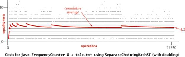
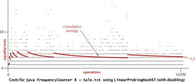
The plots of the cumulative averages for our FrequencyCounter example (shown at the bottom of the previous page) nicely illustrate the dynamic behavior of array resizing in hashing. Each time the array doubles, the cumulative average increases by about 1, because each key in the table needs to be rehashed; then it decreases because about half as many keys hash to each table position, with the rate of decrease slowing as the table fills again.
Memory
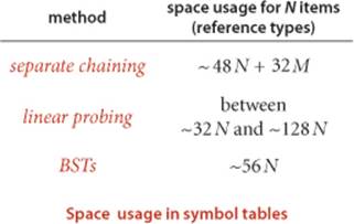
As we have indicated, understanding memory usage is an important factor if we want to tune hashing algorithms for optimum performance. While such tuning is for experts, it is a worthwhile exercise to calculate a rough estimate of the amount of memory required, by estimating the number of references used, as follows: Not counting the memory for keys and values, our implementation SeparateChainingHashST uses memory for M references to SequentialSearchST objects plus M SequentialSearchST objects. Each SequentialSearchST object has the usual 16 bytes of object overhead plus one 8-byte reference (first), and there are a total of N Node objects, each with 24 bytes of object overhead plus 3 references (key, value, and next). This compares with an extra reference per node for binary search trees. With array resizing to ensure that the table is between one-eighth and one-half full, linear probing uses between 4N and 16N references. Thus, choosing hashing on the basis of memory usage is not normally justified. The calculation is a bit different for primitive types (see EXERCISE 3.4.24)
SINCE THE EARLIEST DAYS OF COMPUTING, researchers have studied (and are studying) hashing and have found many ways to improve the basic algorithms that we have discussed. You can find a huge literature on the subject. Most of the improvements push down the space-time curve: you can get the same running time for searches using less space or get faster searches using the same amount of space. Other improvements involve better guarantees, on the expected worst-case cost of a search. Others involve improved hash-function designs. Some of these methods are addressed in the exercises.
Detailed comparison of separate chaining and linear probing depends on myriad implementation details and on client space and time requirements. It is not normally justified to choose separate chaining over linear probing on the basis of performance (see EXERCISE 3.5.31). In practice, the primary performance difference between the two methods has to do with the fact that separate chaining uses a small block of memory for each key-value pair, while linear probing uses two large arrays for the whole table. For huge tables, these needs place quite different burdens on the memory management system. In modern systems, this sort of tradeoff is best addressed by experts in extreme performance-critical situations.
With hashing, under generous assumptions, it is not unreasonable to expect to support the search and insert symbol-table operations in constant time, independent of the size of the table. This expectation is the theoretical optimum performance for any symbol-table implementation. Still, hashing is not a panacea, for several reasons, including:
• A good hash function for each type of key is required.
• The performance guarantee depends on the quality of the hash function.
• Hash functions can be difficult and expensive to compute.
• Ordered symbol-table operations are not easily supported.
Beyond these basic considerations, we defer the comparison of hashing with the other symbol-table methods that we have studied to the beginning of SECTION 3.5.
Q&A
Q. How does Java implement hashCode() for Integer, Double, and Long?
A. For Integer it just returns the 32-bit value. For Double and Long it returns the exclusive or of the first 32 bits with the second 32 bits of the standard machine representation of the number. These choices may not seem to be very random, but they do serve the purpose of spreading out the values.
Q. When using array resizing, the size of the table is always a power of 2. Isn’t that a potential problem, because it only uses the least significant bits of hashCode()?
A. Yes, particularly with the default implementations. One way to address this problem is to first distribute the key values using a prime larger than M, as in the following example:
private int hash(Key x)
{
int t = x.hashCode() & 0x7fffffff;
if (lgM < 26) t = t % primes[lgM+5];
return t % M;
}
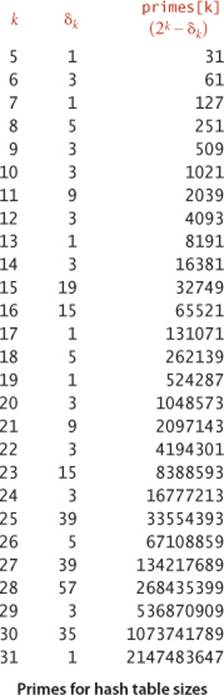
This code assumes that we maintain an instance variable lgM that is equal to lg M (by initializing to the appropriate value, incrementing when doubling, and decrementing when halving) and an array primes[] of the largest prime less than each power of 2 (see the table at right). The constant 5 is an arbitrary choice—we expect the first % to distribute the values equally among the values less than the prime and the second to map about 25 of those values to each value less than M. Note that the point is moot for large M.
Q. I’ve forgotten. Why don’t we implement hash(x) by returning x.hashCode() % M?
A. We need a result between 0 and M-1, but in Java, the % function may be negative.
Q. So, why not implement hash(x) by returning Math.abs(x.hashcode()) % M?
A. Nice try. Unfortunately, Math.abs() returns a negative result for the largest negative number. For many typical calculations, this overflow presents no real problem, but for hashing it would leave you with a program that is likely to crash after a few billion inserts, an unsettling possibility. For example, s.hashCode() is −231 for the Java String value "polygenelubricants". Finding other strings that hash to this value (and to 0) has turned into an amusing algorithm-puzzle pastime.
Q. Do Java library hash functions satisfy ASSUMPTION J?
A. No. For example, the hashCode() implementation in the String data type is not only deterministic but it is specified in the API.
Q. Why not use BinarySearchST or RedBlackBST instead of SequentialSearchST in ALGORITHM 3.5?
A. Generally, we set parameters so as to make the number of keys hashing to each value small, and elementary symbol tables are generally better for the small tables. In certain situations, slight performance gains may be achieved with such hybrid methods, but such tuning is best left for experts.
Q. Is hashing faster than searching in red-black BSTs?
A. It depends on the type of the key, which determines the cost of computing hashCode() versus the cost of compareTo(). For typical key types and for Java default implementations, these costs are similar, so hashing will be significantly faster, since it uses only a constant number of operations. But it is important to remember that this question is moot if you need ordered operations, which are not efficiently supported in hash tables. See SECTION 3.5 for further discussion.
Q. Why not let the linear probing table get, say, three-quarters full?
A. No particular reason. You can choose any value of α, using PROPOSITION M to estimate search costs. For α = 3/4, the average cost of search hits is 2.5 and search misses is 8.5, but if you let α grow to 7/8, the average cost of a search miss is 32.5, perhaps more than you want to pay. As α gets close to 1, the estimate in PROPOSITION M becomes invalid, but you don’t want your table to get that close to being full.
Exercises
3.4.1 Insert the keys E A S Y Q U T I O N in that order into an initially empty table of M = 5 lists, using separate chaining. Use the hash function 11 k % M to transform the kth letter of the alphabet into a table index.
3.4.2 Develop an alternate implementation of SeparateChainingHashST that directly uses the linked-list code from SequentialSearchST.
3.4.3 Modify your implementation of the previous exercise to include an integer field for each key-value pair that is set to the number of entries in the table at the time that pair is inserted. Then implement a method that deletes all keys (and associated values) for which the field is greater than a given integer k. Note: This extra functionality is useful in implementing the symbol table for a compiler.
3.4.4 Write a program to find values of a and M, with M as small as possible, such that the hash function (a * k) % M for transforming the kth letter of the alphabet into a table index produces distinct values (no collisions) for the keys S E A R C H X M P L. The result is known as a perfect hash function.
3.4.5 Is the following implementation of hashCode() legal?
public int hashCode()
{ return 17; }
If so, describe the effect of using it. If not, explain why.
3.4.6 Suppose that keys are t-bit integers. For a modular hash function with prime M, prove that each key bit has the property that there exist two keys differing only in that bit that have different hash values.
3.4.7 Consider the idea of implementing modular hashing for integer keys with the code (a * k) % M, where a is an arbitrary fixed prime. Does this change mix up the bits sufficiently well that you can use nonprime M?
3.4.8 How many empty lists do you expect to see when you insert N keys into a hash table with SeparateChainingHashST, for N=10, 102, 103, 104, 105, and 106? Hint: See EXERCISE 2.5.31.
3.4.9 Implement an eager delete() method for SeparateChainingHashST.
3.4.10 Insert the keys E A S Y Q U T I O N in that order into an initially empty table of size M =16 using linear probing. Use the hash function 11 k % M to transform the kth letter of the alphabet into a table index. Redo this exercise for M = 10.
3.4.11 Give the contents of a linear-probing hash table that results when you insert the keys E A S Y Q U T I O N in that order into an initially empty table of initial size M = 4 that is expanded with doubling whenever half full. Use the hash function 11 k % M to transform the kth letter of the alphabet into a table index.
3.4.12 Suppose that the keys A through G, with the hash values given below, are inserted in some order into an initially empty table of size 7 using a linear-probing table (with no resizing for this problem).
key A B C D E F G
hash (M = 7) 2 0 0 4 4 4 2
Which of the following could not possibly result from inserting these keys?
a. E F G A C B D
b. C E B G F D A
c. B D F A C E G
d. C G B A D E F
e. F G B D A C E
f. G E C A D B F
Give the minimum and the maximum number of probes that could be required to build a table of size 7 with these keys, and an insertion order that justifies your answer.
3.4.13 Which of the following scenarios leads to expected linear running time for a random search hit in a linear-probing hash table?
a. All keys hash to the same index.
b. All keys hash to different indices.
c. All keys hash to an even-numbered index.
d. All keys hash to different even-numbered indices.
3.4.14 Answer the previous question for search miss, assuming the search key is equally likely to hash to each table position.
3.4.15 How many compares could it take, in the worst case, to insert N keys into an initially empty table, using linear probing with array resizing?
3.4.16 Suppose that a linear-probing table of size 106 is half full, with occupied positions chosen at random. Estimate the probability that all positions with indices divisible by 100 are occupied.
3.4.17 Show the result of using the delete() method on page 471 to delete C from the table resulting from using LinearProbingHashST with our standard indexing client (shown on page 469).
3.4.18 Add a constructor to SeparateChainingHashST that gives the client the ability to specify the average number of probes to be tolerated for searches. Use array resizing to keep the average list size less than the specified value, and use the technique described on page 478 to ensure that the modulus for hash() is prime.
3.4.19 Implement keys() for SeparateChainingHashST and LinearProbingHashST.
3.4.20 Add a method to LinearProbingHashST that computes the average cost of a search hit in the table, assuming that each key in the table is equally likely to be sought.
3.4.21 Add a method to LinearProbingHashST that computes the average cost of a search miss in the table, assuming a random hash function. Note: You do not have to compute any hash functions to solve this problem.
3.4.22 Implement hashCode() for various types: Point2D, Interval, Interval2D, and Date.
3.4.23 Consider modular hashing for string keys with R = 256 and M = 255. Show that this is a bad choice because any permutation of letters within a string hashes to the same value.
3.4.24 Analyze the space usage of separate chaining, linear probing, and BSTs for double keys. Present your results in a table like the one on page 476.
Creative Problems
3.4.25 Hash cache. Modify Transaction on page 462 to maintain an instance variable hash, so that hashCode() can save the hash value the first time it is called for each object and does not have to recompute it on subsequent calls. Note: This idea works only for immutable types.
3.4.26 Lazy delete for linear probing. Add to LinearProbingHashST a delete() method that deletes a key-value pair by setting the value to null (but not removing the key) and later removing the pair from the table in resize(). Your primary challenge is to decide when to call resize(). Note: You should overwrite the null value if a subsequent put() operation associates a new value with the key. Make sure that your program takes into account the number of such tombstone items, as well as the number of empty positions, in making the decision whether to expand or contract the table.
3.4.27 Double probing. Modify SeparateChainingHashST to use a second hash function and pick the shorter of the two lists. Give a trace of the process of inserting the keys E A S Y Q U T I O N in that order into an initially empty table of size M =3 using the function 11 k % M (for the kth letter) as the first hash function and the function 17 k % M (for the kth letter) as the second hash function. Give the average number of probes for random search hit and search miss in this table.
3.4.28 Double hashing. Modify LinearProbingHashST to use a second hash function to define the probe sequence. Specifically, replace (i + 1) % M (both occurrences) by (i + k) % M where k is a nonzero key-dependent integer that is relatively prime to M. Note: You may meet the last condition by assuming that M is prime. Give a trace of the process of inserting the keys E A S Y Q U T I O N in that order into an initially empty table of size M =11, using the hash functions described in the previous exercise. Give the average number of probes for random search hit and search miss in this table.
3.4.29 Deletion. Implement an eager delete() method for the methods described in each of the previous two exercises.
3.4.30 Chi-square statistic. Add a method to SeparateChainingHashST to compute the χ2 statistic for the hash table. With N keys and table size M, this number is defined by the equation
χ2 = (M/N) ( (f0 − N/M)2 + (f1 − N/M)2 + . . . + (fM −1 − N/M)2 )
where fi is the number of keys with hash value i. This statistic is one way of checking our assumption that the hash function produces random values. If so, this statistic, for N > cM, should be between ![]() and
and ![]() with probability 1 − 1/c.
with probability 1 − 1/c.
3.4.31 Cuckoo hashing. Develop a symbol-table implementation that maintains two hash tables and two hash functions. Any given key is in one of the tables, but not both. When inserting a new key, hash to one of the tables; if the table position is occupied, replace that key with the new key and hash the old key into the other table (again kicking out a key that might reside there). If this process cycles, restart. Keep the tables less than half full. This method uses a constant number of equality tests in the worst case for search (trivial) and amortized constant time for insert.
3.4.32 Hash attack. Find 2N strings, each of length 2N, that have the same hashCode() value, supposing that the hashCode() implementation for String is the following:
public int hashCode()
{
int hash = 0;
for (int i = 0; i < length(); i ++)
hash = (hash * 31) + charAt(i);
return hash;
}
Strong hint: Aa and BB have the same value.
3.4.33 Bad hash function. Consider the following hashCode() implementation for String, which was used in early versions of Java:
public int hashCode()
{
int hash = 0;
int skip = Math.max(1, length()/8);
for (int i = 0; i < length(); i += skip)
hash = (hash * 37) + charAt(i);
return hash;
}
Explain why you think the designers chose this implementation and then why you think it was abandoned in favor of the one in the previous exercise.
Experiments
3.4.34 Hash cost. Determine empirically the ratio of the time required for hash() to the time required for compareTo(), for as many commonly-used types of keys for which you can get meaningful results.
3.4.35 Chi-square test. Use your solution from EXERCISE 3.4.30 to check the assumption that the hash functions for commonly-used key types produce random values.
3.4.36 List length range. Write a program that inserts N random int keys into a table of size N / 100 using separate chaining, then finds the length of the shortest and longest lists, for N = 103, 104, 105, 106.
3.4.37 Hybrid. Run experimental studies to determine the effect of using RedBlackBST instead of SequentialSearchST to handle collisions in SeparateChainingHashST. This solution carries the advantage of guaranteeing logarithmic performance even for a bad hash function and the disadvantage of necessitating maintenance of two different symbol-table implementations. What are the practical effects?
3.4.38 Separate-chaining distribution. Write a program that inserts 105 random nonnegative integers less than 106 into a table of size 105 using lseparate chaining, and that plots the total cost for each 103 consecutive insertions. Discuss the extent to which your results validate PROPOSITION K.
3.4.39 Linear-probing distribution. Write a program that inserts N/2 random int keys into a table of size N using linear probing, then computes the average cost of a search miss in the resulting table from the cluster lengths, for N = 103, 104, 105, 106. Discuss the extent to which your results validate PROPOSITION M.
3.4.40 Plots. Instrument LinearProbingHashST and SeparateChainingHashST to produce plots like the ones shown in the text.
3.4.41 Double probing. Run experimental studies to evaluate the effectiveness of double probing (see EXERCISE 3.4.27).
3.4.42 Double hashing. Run experimental studies to evaluate the effectiveness of double hashing (see EXERCISE 3.4.28).
3.4.43 Parking problem. (D. Knuth) Run experimental studies to validate the hypothesis that the number of compares needed to insert M random keys into a linear-probing hash table of size M is ~cM3/2, where ![]() .
.
All materials on the site are licensed Creative Commons Attribution-Sharealike 3.0 Unported CC BY-SA 3.0 & GNU Free Documentation License (GFDL)
If you are the copyright holder of any material contained on our site and intend to remove it, please contact our site administrator for approval.
© 2016-2026 All site design rights belong to S.Y.A.