Algorithms in a Nutshell: A Practical Guide (2016)

Chapter 11. Emerging Algorithm Categories

Earlier chapters described algorithms that solve common problems. Obviously, you will encounter challenges in your programming career that do not fit into any common category, so this chapter presents four algorithmic approaches to solving problems.

Another change in this chapter is its focus on randomness and probability. These were used in previous chapters when analyzing the average-case behavior of algorithms. Here the randomness can become an essential part of an algorithm. Indeed, the probabilistic algorithms we describe are interesting alternatives to deterministic algorithms. Running the same algorithm on the same input at two different times may provide very different answers. Sometimes we will tolerate wrong answers or even claims that no solution was found.

Variations on a Theme

The earlier algorithms in this book solve instances of a problem by giving an exact answer on a sequential, deterministic computer. It is interesting to consider relaxing these three assumptions:

Approximation algorithms

Instead of seeking an exact answer for a problem, accept solutions that are close to, but not necessarily as good as, the true answer.

Parallel algorithms

Instead of being restricted to sequential computation, create multiple computational processes to work simultaneously on subproblem instances.

Probabilistic algorithms

Instead of computing the same result for a problem instance, use randomized computations to compute an answer. When run multiple times, the answers often converge on the true answer.

Approximation Algorithms

Approximation algorithms trade off accuracy for more efficient performance. As an example where a “good enough” answer is sufficient, consider the Knapsack Problem, which arises in a variety of computational domains. The goal is to determine the items to add to a backpack that maximize the value of the entire backpack while not exceeding some maximum weight, W. This problem, known as Knapsack 0/1, can be solved using Dynamic Programming. For the Knapsack 0/1 problem, you can only pack one instance of each item. A variation named Knapsack Unbounded allows you to pack as many instances of a particular item that you desire. In both cases, the algorithm must return the maximum value of the items given space constraints.

Consider having the set of four items {4, 8, 9, 10} where each item’s cost in dollars is the same value as its weight in pounds. Thus, the first item weighs 4 pounds and costs $4. Assume the maximum weight you can pack is W = 33 pounds.

As you will recall, Dynamic Programming records the results of smaller subproblems to avoid recomputing them and combines solutions to these smaller problems to solve the original problem. Table 11-1 records the partial results for Knapsack 0/1 and each entry m[i][w] records the maximum value to be achieved by allowing the first i items (the rows below) to be considered with a maximum combined weight of w (the columns below). The maximum value for given weight W using up to four items as shown in the lower-right corner is $31. In this case, one instance of each item is added to the backpack.

For the Knapsack Unbounded variation, Table 11-2 records the entry m[w], which represents the maximum value attained for weight w if you are allowed to pack any number of instances of each item. The maximum value for given weight W as shown in the rightmost entry below is $33. In this case, there are six instances of the four-pound item and one nine-pound item.

KNAPSACK 0/1 SUMMARY

Best, Average, Worst: O(n*W)

Knapsack 0/1 (weights, values, W)

n = number of items

m = empty (n+1) x (W+1) matrix

for i=1 to n do

for j=0 to W do

if weights[i-1] <= j then

remaining = j - weights[i-1]

m[i][j] = max(m[i-1][j], m[i-1][remaining] + values[i-1])

else

m[i][j] = m[i-1][j]

return m[n][W]

end

Knapsack unbounded(weights, values, W)

n = number of items

m = empty (W+1) vector

for j=1 to W+1 do

best = m[j-1]

for i=0 to n-1 do

remaining = j - weights[i]

if remaining >= 0 andm[remaining] + values[i] > best then

best = m[remaining] + values[i]

m[j] = best

return m[W]

m[i][j] records maximum value using first i items without exceeding weight j.

Can we increase value by adding item i – 1 to previous solution with weight (j – that item’s weight)?

Item i – 1 exceeds weight limit and thus can’t improve solution.

Return computed best value.

For unbounded, m[j] records maximum value without exceeding weight j.

Input/Output

You are given a set of items (each with an integer weight and value) and a maximum weight, W. The problem is to determine which items to pack into the knapsack so the total weight is less than or equal to W and the total value of the packed items is as large as possible.

Context

This is a type of resource allocation problem with constraints that is common in computer science, mathematics, and economics. It has been studied extensively for over a century and has numerous variations. Often you need to know the actual selection of items, not just the maximum value, so the solution must also return the items selected to put into the knapsack.

Solution

We use Dynamic Programming, which works by storing the results of simpler subproblems. For Knapsack 0/1, the two-dimensional matrix m[i][j] records the result of the maximum value using the first i items without exceeding weight j. The structure of the solution in Example 11-1matches the expected double loops of Dynamic Programming.

Example 11-1. Python implementation of Knapsack 0/1

class Item:

def __init__(self, value, weight):

"""Create item with given value and weight."""

self.value = value

self.weight = weight

def knapsack_01 (items, W):

"""

Compute 0/1 knapsack solution (just one of each item is available)

for set of items with corresponding weights and values. Return total

weight and selection of items.

"""

n = len(items)

m = [None] * (n+1)

for i inrange(n+1):

m[i] = [0] * (W+1)

for i inrange(1,n+1):

for j inrange(W+1):

if items[i-1].weight <= j:

valueWithItem = m[i-1][j-items[i-1].weight] + items[i-1].value

m[i][j] = max(m[i-1][j], valueWithItem)

else:

m[i][j] = m[i-1][j]

selections = [0] * n

i = n

w = W

while i > 0 andw >= 0:

if m[i][w] != m[i-1][w]:

selections[i-1] = 1

w -= items[i-1].weight

i -= 1

return (m[n][W], selections)

This code follows the Dynamic Programming structure by computing each subproblem in order. Once the nested for loops compute the maximum value, m[n][W], the subsequent while loop shows how to recover the actual items selected by “walking” over the m matrix. It starts at the lower righthand corner, m[n][W], and determines whether the i^th item was selected, based on whether m[i][w] is different from m[i-1][w]. If this is the case, it records the selection and then moves left in m by removing the weight of i and continuing until it hits the first row (no more items) or the left column (no more weight); otherwise it tries the previous item.

The Knapsack Unbounded problem uses a one-dimensional vector m[j] to record the result of the maximum value not exceeding weight j. Its Python implementation is shown in Example 11-2.

Example 11-2. Python implementation of Knapsack unbounded

def knapsack_unbounded (items, W):

"""

Compute unbounded knapsack solution (any number of each item is

available) for set of items with corresponding weights and values.

Return total weight and selection of items.

"""

n = len(items)

progress = [0] * (W+1)

progress[0] = -1

m = [0] * (W + 1)

for j inrange(1, W+1):

progress[j] = progress[j-1]

best = m[j-1]

for i inrange(n):

remaining = j - items[i].weight

if remaining >= 0 andm[remaining] + items[i].value > best:

best = m[remaining] + items[i].value

progress[j] = i

m[j] = best

selections = [0] * n

i = n

w = W

while w >= 0:

choice = progress[w]

if choice == -1:

break

selections[choice] += 1

w -= items[progress[w]].weight

return (m[W], selections)

Analysis

These solutions are not O(n) as one might expect, because that would require the overall execution to be bounded by c*n, where c is a constant for sufficiently large n. The execution time depends on W as well. That is, in both cases, the solution is O(n*W), as clearly shown by the nested forloops. Recovering the selections is O(n), so this doesn’t change the overall performance.

Why does this observation matter? In Knapsack 0/1, when W is much larger than the weights of the individual items, the algorithm must repeatedly perform wasted iterations, because each item is only chosen once. There are similar inefficiencies for Knapsack Unbounded.

In 1957, George Dantzig proposed an approximate solution to Knapsack Unbounded, shown in Example 11-3. The intuition behind this approximation is that you should first insert items into the knapsack that maximize the value-to-weight ratio. In fact, this approach is guaranteed to find an approximation that is no worse than half of the maximum value that would have been found by Dynamic Programming. In practice, the results are actually quite close to the real value, and the code is noticeably faster.

Example 11-3. Python implementation of Knapsack unbounded approximation

class ApproximateItem(Item):

"""

Extends Item by storing the normalized value and the original position

of the item before sorting.

"""

def __init__(self, item, idx):

Item.__init__(self, item.value, item.weight)

self.normalizedValue = item.value/item.weight

self.index = idx

def knapsack_approximate (items, W):

"""Compute approximation to knapsack problem using Dantzig approach."""

approxItems = []

n = len(items)

for idx inrange(n):

approxItems.append (ApproximateItem(items[idx], idx))

approxItems.sort (key=lambda x:x.normalizedValue, reverse=True)

selections = [0] * n

w = W

total = 0

for idx inrange(n):

item = approxItems[idx]

if w == 0:

break

# find out how many fit

numAdd = w // item.weight

if numAdd > 0:

selections[item.index] += numAdd

w -= numAdd * item.weight

total += numAdd * item.value

return (total, selections)

The implementation iterates over the items in reverse order by their normalized value (i.e., the ratio of value to weight). The cost of this algorithm is O(n log n) because it must sort the items first.

Returning to the original set of four items {4, 8, 9, 10} in our earlier example, observe that the ratio of value to weight is 1.0 for each item, which means they are all “equivalent” in importance according to the algorithm. For the given weight W = 33, the approximation chooses to pack eight instances of the item weighing four pounds, which results in a total value of $32. It is interesting that all three algorithms came up with a different value given the same items and overall weight constraint.

The following table compares the performance of the Knapsack Unbounded Approximation with Knapsack Unbounded as W grows in size. Each of the items in the set of n = 53 items has a different weight and each item’s value is set to its weight. The weights range from 103 to 407. As you can see, as the size of W doubles, the time to execute Knapsack Unbounded also doubles, because of its O(n*W) performance. However, the performance of Knapsack Approximate doesn’t change as W gets larger because its performance is determined only by O(n log n).

Reviewing the final two columns, you can see that for W = 175, the approximate solution is 60% of the actual answer. As W increases, the approximate solution converges to be closer to the actual answer. Also, the approximation algorithm is almost 1,000 times faster.

Parallel Algorithms

Parallel algorithms take advantage of existing computational resources by creating and managing different threads of execution.

Quicksort, presented in Chapter 4, can be implemented in Java as shown in Example 11-4, assuming the existence of a partition function to divide the original array into two subarrays based on a pivot value. As you recall from Chapter 4, values to the left of pivotIndex are ≤ the pivot value while values to the right of pivotIndex are ≥ the pivot value.

Example 11-4. Quicksort implementation in Java

public class MultiThreadQuickSort<E extends Comparable<E>> {

final E[] ar; /** Elements to be sorted. */

IPivotIndex pi; /** Partition function. */

/** Construct an instance to solve quicksort. */

public MultiThreadQuickSort (E ar[]) {

this.ar = ar;

}

/** Set the partition method. */

public void setPivotMethod (IPivotIndex ipi) { this.pi = ipi; }

/** Single-thread sort of ar[left,right]. */

public void qsortSingle (int left, int right) {

if (right <= left) { return; }

int pivotIndex = pi.selectPivotIndex (ar, left, right);

pivotIndex = partition (left, right, pivotIndex);

qsortSingle (left, pivotIndex-1);

qsortSingle (pivotIndex+1, right);

}

}

The two subproblems qsortSingle (left, pivotIndex-1) and qsortSingle (pivotIndex+1, right) are independent problems and, theoretically, can be solved at the same time. The immediate question is how to use multiple threads to solve this problem. You cannot simply spawn a helper thread with each recursive call since that would overwhelm the resources of the operating system. Consider the rewrite, qsort2, shown in Example 11-5:

Example 11-5. Multithreaded Java Quicksort implementation

/** Multi-thread sort of ar[left,right]. */

void qsort2 (int left, int right) {

if (right <= left) { return; }

int pivotIndex = pi.selectPivotIndex (ar, left, right);

pivotIndex = partition (left, right, pivotIndex);

qsortThread (left, pivotIndex-1);

qsortThread (pivotIndex+1, right);

}

/**

* Spawn thread to sort ar[left,right] or use existing thread

* if problem size is too big or all helpers are being used.

*/

private void qsortThread (final int left, final int right) {

// are all helper threads working OR is problem too big?

// Continue with recursion if so.

int n = right + 1 - left;

if (helpersWorking == numThreads || n >= threshold) {

qsort2 (left, right);

} else {

// otherwise, complete in separate thread

synchronized (helpRequestedMutex) {

helpersWorking++;

}

new Thread () {

public void run () {

// invoke single-thread qsort

qsortSingle (left, right);

synchronized (helpRequestedMutex) {

helpersWorking--;

}

}

}.start();

}

}

For each of the two qsortThread subproblems, there is a simple check to see whether the primary thread should continue the recursive qsortThread function call. The separate helper thread is dispatched to compute a subproblem only if a thread is available and the size of the subproblem is smaller than the specified threshold value. This logic is applied when sorting the left subarray as well as the right subarray. The threshold value is computed by calling setThresholdRatio(r), which sets the threshold problem size to be n/r where n is the number of elements to be sorted. The default ratio is 5, which means a helper thread is only invoked on subproblems that are smaller than 20% of the original problem size.

The helpersWorking class attribute stores the number of active helper threads. Whenever a thread is spawned, the helpersWorking variable is incremented, and the thread itself will decrement this same value on completion. Using the mutex variable, helpRequestedMutex, and the ability in Java to synchronize a block of code for exclusive access, this implementation safely updates the helpersWorking variable. qsort2 invokes the single-threaded qsortSingle method within its helper threads. This ensures only the primary thread is responsible for spawning new threads of computation.

For this design, helper threads cannot spawn additional helper threads. If this were allowed to happen, the “first” helper thread would have to synchronize with these “second” threads, so the “second” threads would only begin to execute after the “first” helper thread had properly partitioned the array.

Figures 11-1 and 11-2 compare the Java single-helper solution against a single-threaded solution sorting random integers from the range [0, 16777216]. We consider several parameters:

Size n of the array being sorted

This falls in the range {65,536 to 1,048,576}.

Threshold n/r

This determines the maximum size of the problem for which a helper thread is spawned. We experimented with values of r in the range {1 to 20} and MAXINT, which effectively denies using helper threads.

Number of helper threads available

We experimented with 0 to 9 helper threads.

Partition method to use

We tried both “select a random element” and “select the rightmost element.”

The parameter space thus amounts to 2,000 unique combinations of these parameters. In general, we found there is a noticeable performance slowdown of about 5% in using the random number generator across all experiments, so we now focus only on the “rightmost” partition method. In addition, for Quicksort, having more than one helper thread available did not improve the performance, so we focus only on having a single helper thread.

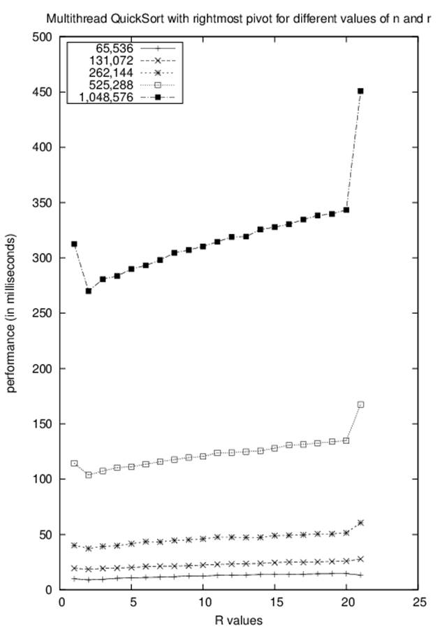
Figure 11-1. Multithreaded Quicksort for varying n and r

Reading the graph from left to right, you can see that the first data point (r = 1) reports the performance that tries to immediately begin using the helper thread, while the last data point (r = 21) reports the result when no helper thread is ever used. When we compute the speedup factor from time T1 to a smaller time T2, we use the equation T1/T2. Simply using an extra thread shows a speedup factor of about 1.3. This is a very nice return on investment for a small programming change, as shown in Table 11-4.

Returning to Figure 11-1, you can see that the best improvement occurs near where r = 2. There is a built-in overhead to using threads, and we shouldn’t automatically dispatch a new thread of execution without some assurance that the primary thread will not have to wait and block until the helper thread completes its execution. These results will differ based on the computing platform used.

In many cases, the speedup is affected by the number of CPUs on the computing platform. Figure 11-2 contains the speedup tables on two different computing platforms—a dual-core CPU and a quad-core CPU. Each row represents the potential number of available threads while each column represents a threshold value r. The total number of elements sorted is fixed at n = 1,048,576. The quad-core results demonstrate the effectiveness of allowing multiple threads, achieving a speedup of 1.5; the same cannot be said of the dual-core execution, whose performance increases by no more than 5% when allowing multiple threads.

Research in speedup factors for parallel algorithms shows there are inherent limitations to how much extra threading or extra processing will actually help a specific algorithmic implementation. Here the multithreaded Quicksort implementation achieves a nice speedup factor because the individual subproblems of recursive Quicksort are entirely independent; there will be no contention for shared resources by the multiple threads. If other problems share this same characteristic, they should also be able to benefit from multithreading.

Probabilistic Algorithms

A probabilistic algorithm uses a stream of random bits (i.e., random numbers) as part of the process for computing an answer, so you will get different results when running the algorithm on the same problem instance. Often, assuming access to a stream of random bits leads to algorithms that are faster than any current alternatives.

For practical purposes, we should be aware that streams of random bits are very difficult to generate on deterministic computers. Though we may generate streams of quasi-random bits that are virtually indistinguishable from streams of truly random bits, the cost of generating these streams should not be ignored.

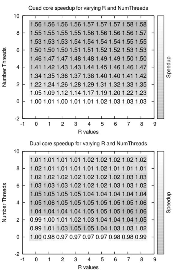
Figure 11-2. Performance of multithreaded Quicksort with fixed n and varying r and number of threads

Estimating the Size of a Set

As an example of the speedup that can be obtained in allowing probabilistic algorithms, assume we want to estimate the size of a set of n distinct objects (i.e., we want to estimate the value n by observing individual elements). It would be straightforward to count all the objects, at a cost of O(n). Clearly this process is guaranteed to yield an exact answer. But if an incorrect estimate of the value of n is tolerable, assuming it could be computed more quickly, the algorithm described in Example 11-6 is a faster alternative. This algorithm is similar to the mark-and-recapture experiments biologists use to estimate the size of a spatially limited population of organisms. The approach here is to use a generator function that returns a random individual in the population.

Example 11-6. Implementation of probabilistic counting algorithm

def computeK(generator):

"""

Compute estimate of using probabilistic counting algorithm.

Doesn't know value of n, the size of the population.

"""

seen = set()

while True:

item = generator()

if item inseen:

k = len(seen)

return 2.0*k*k/math.pi

else:

seen.add(item)

Let’s start with some intuition. We must have the ability to pick random elements from the set and mark them as being seen. Since we assume the set is finite, at some point we must eventually select an element that we have seen before. The longer it takes to choose a previously selected element, the larger the size of the original set must be. In statistics, this behavior is known as “sampling with replacement” and the expected number of selections, k, we can make until seeing a previously selected element is

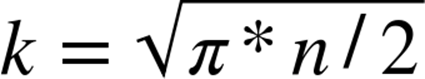
As long as the generator function returns an element that has already been seen (which it must do because the population is finite) the while loop will terminate after some number of selections, k. Once k is computed, rearrange the preceding formula to compute an approximation of n. Clearly, the algorithm can never give the exact value of n, because 2*k²/π can never be an integer, but this computation is an unbiased estimate of n.

In Table 11-5 we show a sample run of the algorithm that records the results of performing the computation repeatedly for a number of trials, t = {32, 64, 128, 256, 512}. From these trials, the lowest and highest estimates were discarded, and the average of the remaining t-2 trials is shown in each column.

Because of the random nature of the trials, it is not at all guaranteed that the final accurate result can be achieved simply by averaging over an increasing number of independent random trials. Even increasing the number of trials does little to improve the accuracy, but that misses the point; this probabilistic algorithm efficiently returns an estimate based on a small sample size.

Estimating the Size of a Search Tree

Mathematicians have long studied the 8-Queens Problem, which asks whether it is possible to place eight queens on a chessboard so that no two queens threaten each other. This was expanded to the more general problem of counting the number of unique solutions to placing nnonthreatening queens on an n-by-n chessboard. No one has yet been able to devise a way to mathematically compute this answer; instead you can write a brute-force program that checks all possible board configurations to determine the answer. Table 11-6 contains some of the computed values taken from the On-Line Encyclopedia of Integer Sequences. As you can see, the number of solutions grows extremely rapidly.

To count the number of exact solutions to the 4-Queens Problem, we expand a search tree (shown in Figure 11-3) based on the fact that each solution will have one queen on each row. Such an exhaustive elaboration of the search tree permits us to see that there are two solutions to the 4-Queens Problem. Trying to compute the number of solutions to the 19-Queens Problem is much harder because there are 4,968,057,848 nodes at level 19 of the search tree. It is simply prohibitively expensive to generate each and every solution.

However, what if you were interested only in approximating the number of solutions, or in other words, the number of potential board states on level n? Knuth (1975) developed a novel alternative approach to estimate the size and shape of a search tree. His method corresponds to taking a random walk down the search tree. For the sake of brevity, we illustrate his technique for the 4-Queens Problem, but clearly it could just as easily be applied to approximate the number of solutions to the 19-Queens Problem. Instead of counting all possible solutions, create a single board state containing n queens and estimate the overall count by totaling the potential board states not followed, assuming each of these directions would be equally productive.

Figure 11-4 demonstrates Knuth’s approach on a 4x4 chessboard. Each of the board states has an associated estimate in a small circle for the number of board states in the entire tree at that level. Starting with the root of the search tree (no queens placed), each board state expands to a new level based on its number of children. We will conduct a large number of random walks over this search tree, which will never be fully constructed during the process. In each walk we will select moves at random until a solution is reached or no moves are available. By averaging the number of solutions returned by each random walk, we can approximate the actual count of states in the tree. Let’s perform two possible walks starting from the root node at level 0:

§ Choose the leftmost board state in the first level. Because there are four children, our best estimate for the total number of states at level 1 is 4. Now again, choose the leftmost child from its two children, resulting in a board state on level 2. From its perspective, assuming each of the other three children of the root node are similarly productive, it estimates the total number of board states on level 2 to be 4*2 = 8. However, at this point, there are no more possible moves, so from its perspective, it assumes no other branch is productive, so it estimates there are 0 board states at level 3 and the search terminates with no solution found.

§ Choose the second-to-left board state in the first level. Its best estimate for the number of states at level 1 is 4. Now, in each of the subsequent levels there is only one valid board state, which leads to the estimate of 4*1 = 4 for the number of board states at each subsequent level, assuming all of the other original paths were similarly productive. Upon reaching the lowest level, it estimates there are four solutions in the entire tree.

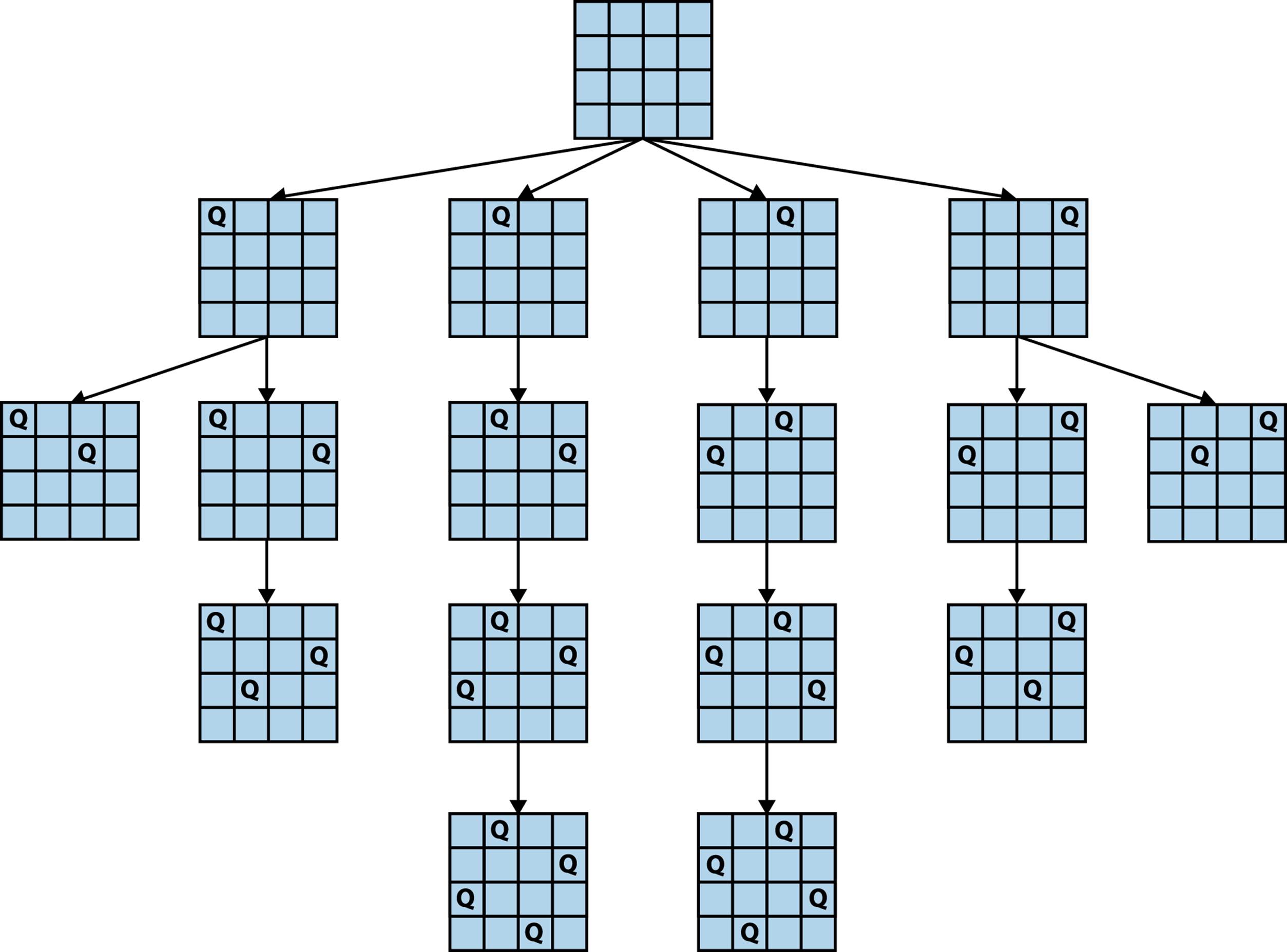
Figure 11-3. Final solution for 4-Queens Problem with four rows extended

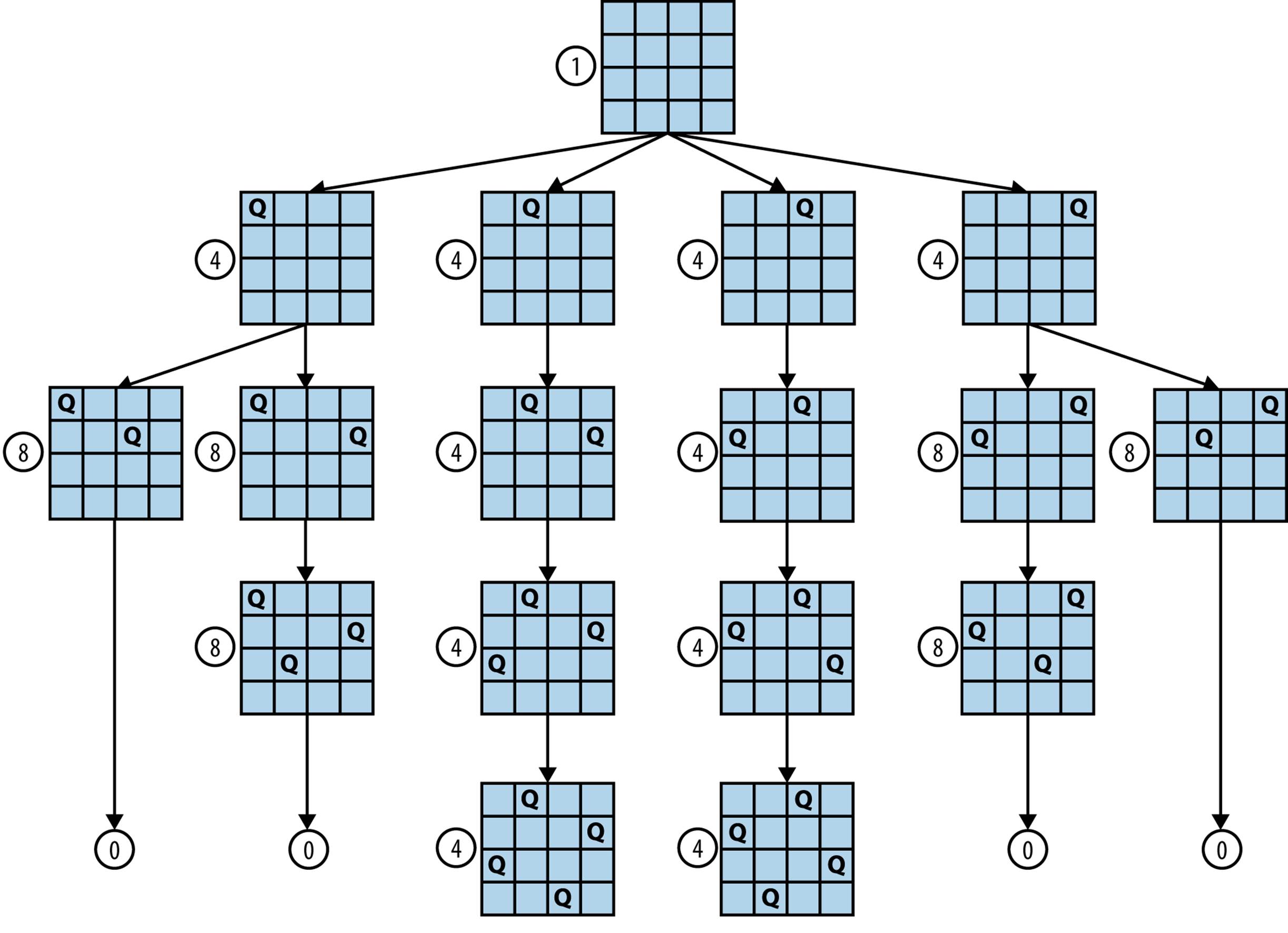
Figure 11-4. Estimating number of solutions of 4-Queens Problem

Neither of these estimates is correct, and it is typical of this approach that different walks lead to under- and overestimates of the actual count. However, if we perform a large number of random walks, the average of the estimates will converge on the value. Each estimate can be computed quickly, thus this refined (averaged) estimate can also be computed quickly.

If you refer back to Table 11-6, we show the computed results from our implementation for 1,024, 8,192, and 65,536 trials. No timing information is included, because all results were computed in less than a minute. The final estimate for the 19-Queens problem with T = 65,536 trials is within 3% of the actual answer. Indeed, all of the estimates for T = 65,536 are within 5.8% of the actual answer. This algorithm has the desirable property that the computed value is more accurate as more random trials are run. Example 11-7 shows the implementation in Java for a single estimate of the n-Queens problem.

Example 11-7. Implementation of Knuth’s randomized estimation of n-Queens problem

/**

* For an n-by-n board, store up to n nonthreatening queens and

* search along the lines of Knuth's random walk. It is assumed the

* queens are being added row by row starting from 0.

*/

public class Board {

boolean [][] board; /** The board. */

final int n; /** board size. */

/** Temporary store for last valid positions. */

ArrayList<Integer> nextValidRowPositions = new ArrayList<Integer>();

public Board (int n) {

board = new boolean[n][n];

this.n = n;

}

/** Start with row and work upwards to see if still valid. */

private boolean valid (int row, int col) {

// another queen in same column, left diagonal, or right diagonal?

int d = 0;

while (++d <= row) {

if (board[row-d][col]) { return false; }

if (col >= d && board[row-d][col-d]) { return false; }

if (col+d < n && board[row-d][col+d]) { return false; }

}

return true; // OK

}

/**

* Find out how many valid children states are found by trying to add

* a queen to the given row. Returns a number from 0 to n.

*/

public int numChildren (int row) {

int count = 0;

nextValidRowPositions.clear();

for (int i = 0; i < n; i++) {

board[row][i] = true;

if (valid (row, i)) {

count++;

nextValidRowPositions.add (i);

}

board[row][i] = false;

}

return count;

}

/** If no board is available at this row then return false. */

public boolean randomNextBoard (int r) {

int sz = nextValidRowPositions.size();

if (sz == 0) { return false; }

// select one randomly

int c = (int) (Math.random()*sz);

board[r][nextValidRowPositions.get (c)] = true;

return true;

}

}

public class SingleQuery {

/** Generate table. */

public static void main (String []args) {

for (int i = 0; i < 100; i++) {

System.out.println(i + ": " + estimate(19));

}

}

public static long estimate (int n) {

Board b = new Board(n);

int r = 0;

long lastEstimate = 1;

while (r < n) {

int numChildren = b.numChildren (r);

// no more to go, so no solution found.

if (!b.randomNextBoard (r)) {

lastEstimate = 0;

break;

}

// compute estimate based on ongoing tally and advance

lastEstimate = lastEstimate*numChildren;

r++;

}

return lastEstimate;

}

}

References

Armstrong, J., Programming Erlang: Software for a Concurrent World. Second Edition. Pragmatic Bookshelf, 2013.

Berman, K. and J. Paul, Algorithms: Sequential, Parallel, and Distributed. Course Technology, 2004.

Christofides, N., “Worst-case analysis of a new heuristic for the traveling salesman problem,” Report 388, Graduate School of Industrial Administration, CMU, 1976.

Knuth, D. E., “Estimating the efficiency of backtrack programs,” Mathematics of Computation, 29(129): 121–136, 1975.