Algorithms in a Nutshell: A Practical Guide (2016)

Chapter 10. Spatial Tree Structures

The algorithms in this chapter are concerned primarily with modeling two-dimensional structures over the Cartesian plane to conduct powerful search queries that go beyond simple membership, as covered in Chapter 5. These algorithms include:

Nearest neighbor

Given a set of two-dimensional points, P, determine which point is closest to a target query point, x. This can be solved in O(log n) instead of an O(n) brute-force solution.

Range queries

Given a set of two-dimensional points, P, determine which points are contained within a given rectangular region. This can be solved in O(n^0.5 + r) where r is the number of reported points, instead of an O(n) brute-force solution.

Intersection queries

Given a set of two-dimensional rectangles, R, determine which rectangles intersect a target rectangular region. This can be solved in O(log n) instead of an O(n) brute-force solution.

Collision detection

Given a set of two-dimensional points, P, determine the intersections between squares of side s centered on these points. This can be solved in O(n log n) instead of an O(n²) brute-force solution.

The structures and algorithms naturally extend to multiple dimensions, but this chapter will remain limited to two-dimensional structures for convenience. The chapter is named after the many ways researchers have been able to partition n-dimensional data using the intuition at the heart of binary search trees.

Nearest Neighbor Queries

Given a set of points, P, in a two-dimensional plane, you might need to determine the point in P that is closest to a query point x using Euclidean distance. Note that point x does not have to already exist in P, which differentiates this problem from the searching algorithms from Chapter 5. These queries also extend to input sets whose points are found in n-dimensional space.

The naïve implementation is to inspect all points in P, resulting in a linear O(n) algorithm. Because P is known in advance, perhaps there is some way to structure its information to speed up queries by discarding large groups of its points during the search. Perhaps we could partition the plane into bins of some fixed size m by m, as shown in Figure 10-1(a). Here 10 input points in P (shown as circles) are placed into nine enclosing bins. The large shaded number in each bin reflects the number of points in it. When searching for the closest neighbor for a point x (shown as a small black square), find its enclosing bin. If that bin is not empty, we only need to search the bins that intersect the focus circle whose radius is m*sqrt(2).

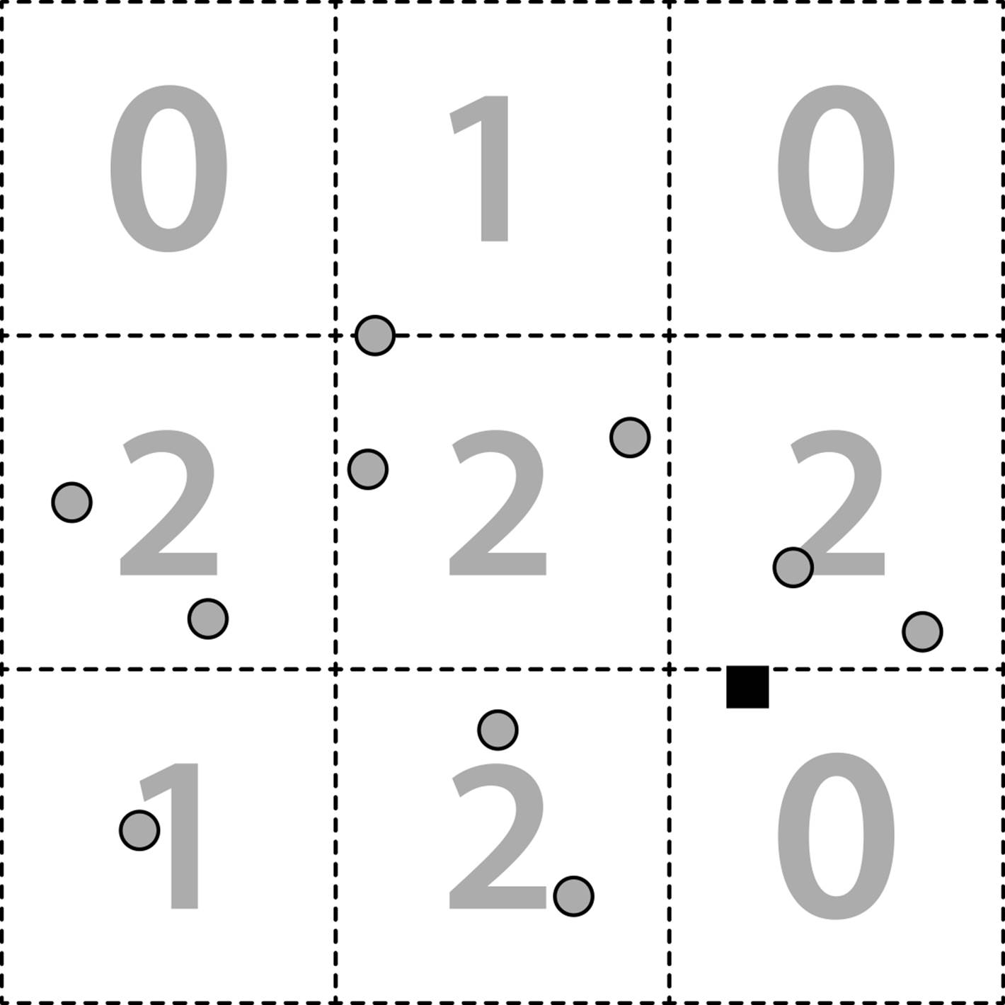
Figure 10-1. Bin approach for locating nearest neighbor

In this example, however, there are no points in the target bin, and the three neighboring bins will need to be examined. This ineffective approach is inappropriate because many bins may in fact be empty, and the algorithm would still have to search multiple neighboring bins. As we saw inChapter 5, binary search trees reduce the effort by eliminating from consideration groups of points that could not be part of the solution. In this chapter, we introduce the idea of a spatial tree to partition the points in the two-dimensional plane to reduce the search time. The extra cost of preprocessing all points in P into an efficient structure is recouped later by savings of the query computations, which become O(log n). If the number of searches is small, then the brute-force O(n) comparison is best.

Range Queries

Instead of searching for a specific target point, a query could instead request all points in P that are contained within a given rectangular region of the two-dimensional plane. The brute-force solution checks whether each point is contained within the target rectangular region, resulting in O(n) performance.

The same data structure developed for nearest-neighbor queries also supports these queries, known as the “orthogonal range,” because the rectangular query region is aligned with the x and y axes of the plane. The only way to produce better than O(n) performance is to find a way to both discard points from consideration, and include points in the query result. Using a k-d tree, the query is performed using a recursive traversal, and the performance can be O(n^0.5 + r), where r is the number of points reported by the query.

Intersection Queries

The input set being searched can typically be more complicated than a single n-dimensional point. Consider instead a set of rectangles R in a two-dimensional plane where each rectangle r_i is defined by a tuple (x_low, y_low, x_high, y_high). With this set R you might want to locate all rectangles that intersect a given point (x, y) or (more generally) intersect a target rectangle (x₁, y₁, x₂, y₂). Structuring the rectangles appears to be more complicated because the rectangles can overlap each other in the plane.

Instead of providing a target rectangle, we might be interested in identifying the intersections among a collection of two-dimensional elements. This is known as the collision detection problem, and we present a solution to detect intersections among a collection of points, P, using square-based regions centered around each point.

Spatial Tree Structures

Spatial tree structures show how to represent data to efficiently support the execution of these three common searches. In this chapter, we present a number of spatial tree structures that have been used to partition n-dimensional objects to improve the performance of search, insert, and delete operations. We now present three such structures.

k-d Tree

In Figure 10-2(a), the same 10 points from Figure 10-1 are shown in a k-d tree, so named because it can subdivide a k-dimensional plane along the perpendicular axes of the coordinate system. These points are numbered in the order in which they were inserted into the tree. The structure of the k-d tree from Figure 10-2(a) is depicted as a binary tree in Figure 10-2(b). For the remainder of this discussion we assume a two-dimensional tree, but the approach can also be used for arbitrary dimensions.

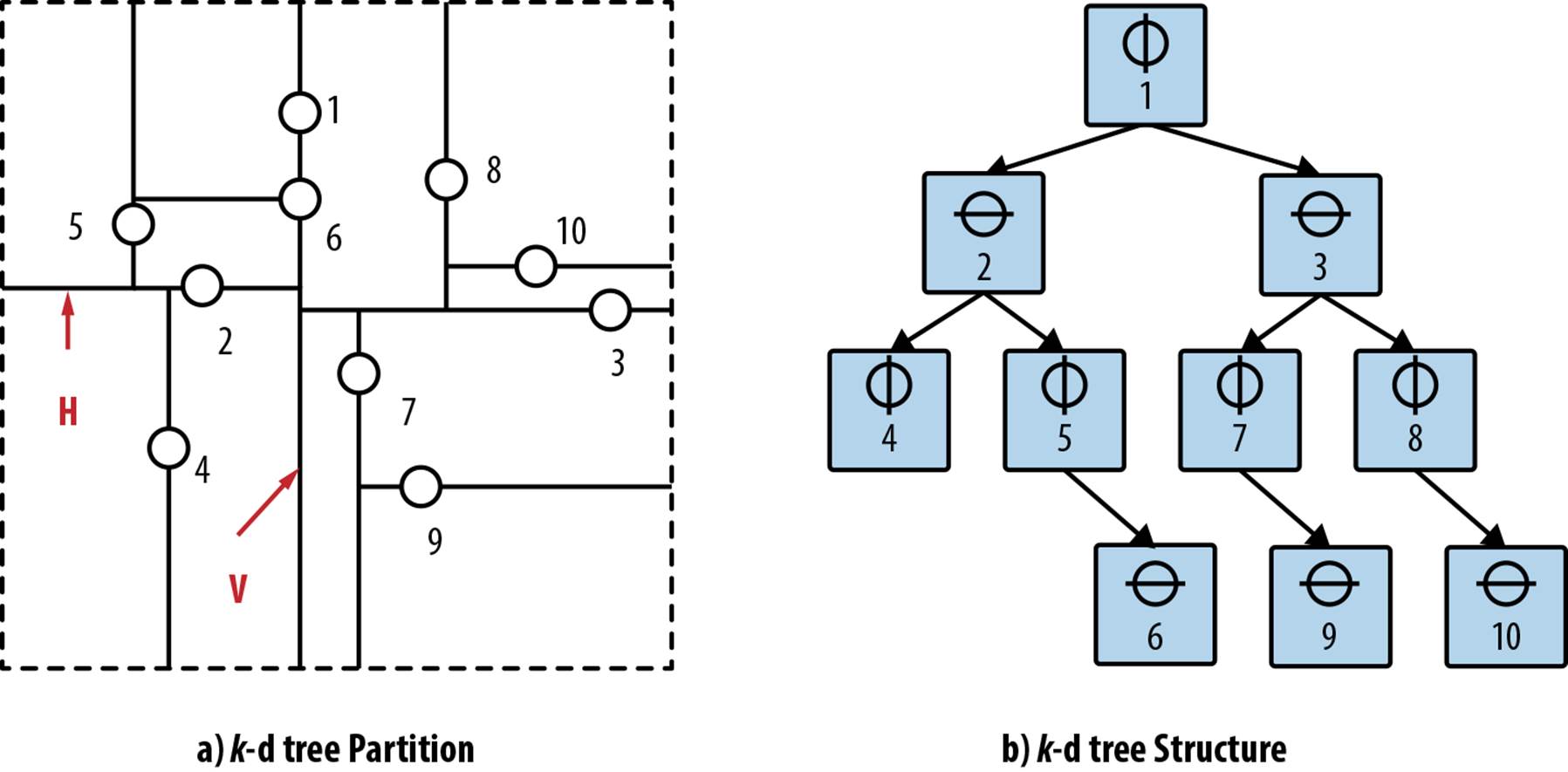
Figure 10-2. Division of two-dimensional plane using k-d tree

A k-d tree is a recursive binary tree structure where each node contains a point and a coordinate label (i.e., either x or y) that determines the partitioning orientation. The root node represents the rectangular region (x_low = –∞, y_low = –∞, x_high = +∞, y_high = +∞) in the plane partitioned along the vertical line V through point p₁. The left subtree further partitions the region to the left of V, whereas the right subtree further partitions the region to the right of the V. The left child of the root represents a partition along the horizontal line H through p₂ that subdivides the region to the left ofV into a region above the line H and a region below the line H. The region (–∞, –∞, p₁.x, +∞) is associated with the left child of the root, whereas the region (p₁.x, ≠∞, +∞, +∞) is associated with the right child of the root. These regions are effectively nested, and we can see that the region of an ancestor node wholly contains the regions of any of its descendant nodes.

Quadtree

A quadtree partitions a set of two-dimensional points, P, recursively subdividing the overall space into four quadrants. It is a tree-like structure where each nonleaf node has four children, labeled NE (NorthEast), NW (NorthWest), SW (SouthWest), and SE (SouthEast). There are two distinct flavors of quadtrees:

Region-based

Given a 2^k by 2^k image of pixels where each pixel is 0 or 1, the root of a quadtree represents the entire image. Each of the four children of the root represents a 2^k–1 by 2^k–1 quadrant of the original image. If one of these four regions is not entirely 0s or 1s, then the region is subdivided into subregions, each of which is one-quarter the size of its parent. Leaf nodes represent a square region of pixels that are all 0s or 1s. Figure 10-3 describes the tree structure with a sample image bitmap.

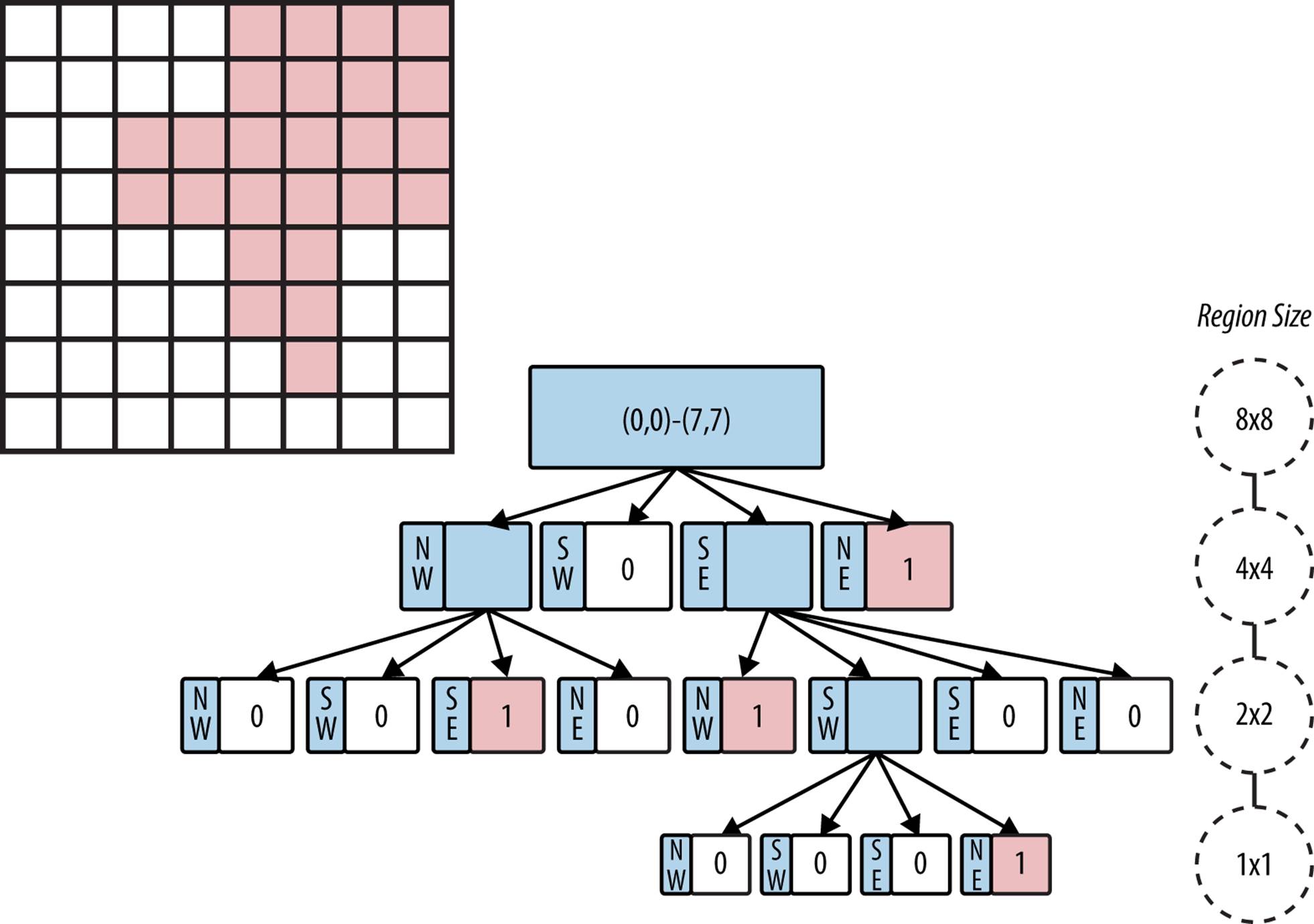
Figure 10-3. Quadtree using region-based partitioning

Point-based

Given a 2^k by 2^k space in the Cartesian plane, the quadtree directly maps to a binary tree structure, where each node can store up to four points. If a point is added to a full region, the region is subdivided into four regions each one-quarter the size of its parent. When no points are present in a quadrant for a node, then there is no child node for that quadrant, and so the shape of the tree depends on the order the points were added to the quadtree.

For this chapter, we focus on point-based quadtrees. Figure 10-4 shows an example containing 13 points in a 256 by 256 region. The quadtree structure is shown on the right side of the image. Note that there are no points in the root’s SouthEast quadrant, so the root only has three children nodes. Also note the variable subdivisions of the regions based on which points have been added to the quadtree.

R-Tree

An R-Tree is a tree structure in which each node contains up to M links to children nodes. All actual information is stored by the leaf nodes, each of which can store up to M different rectangles. Figure 10-5 depicts an R-Tree where M = 4 and six rectangles have been inserted (labeled 1, 2, 3, 4, 5, and 6). The result is the tree shown on the right where the interior nodes reflect different rectangular regions inside of which the actual rectangles exist.

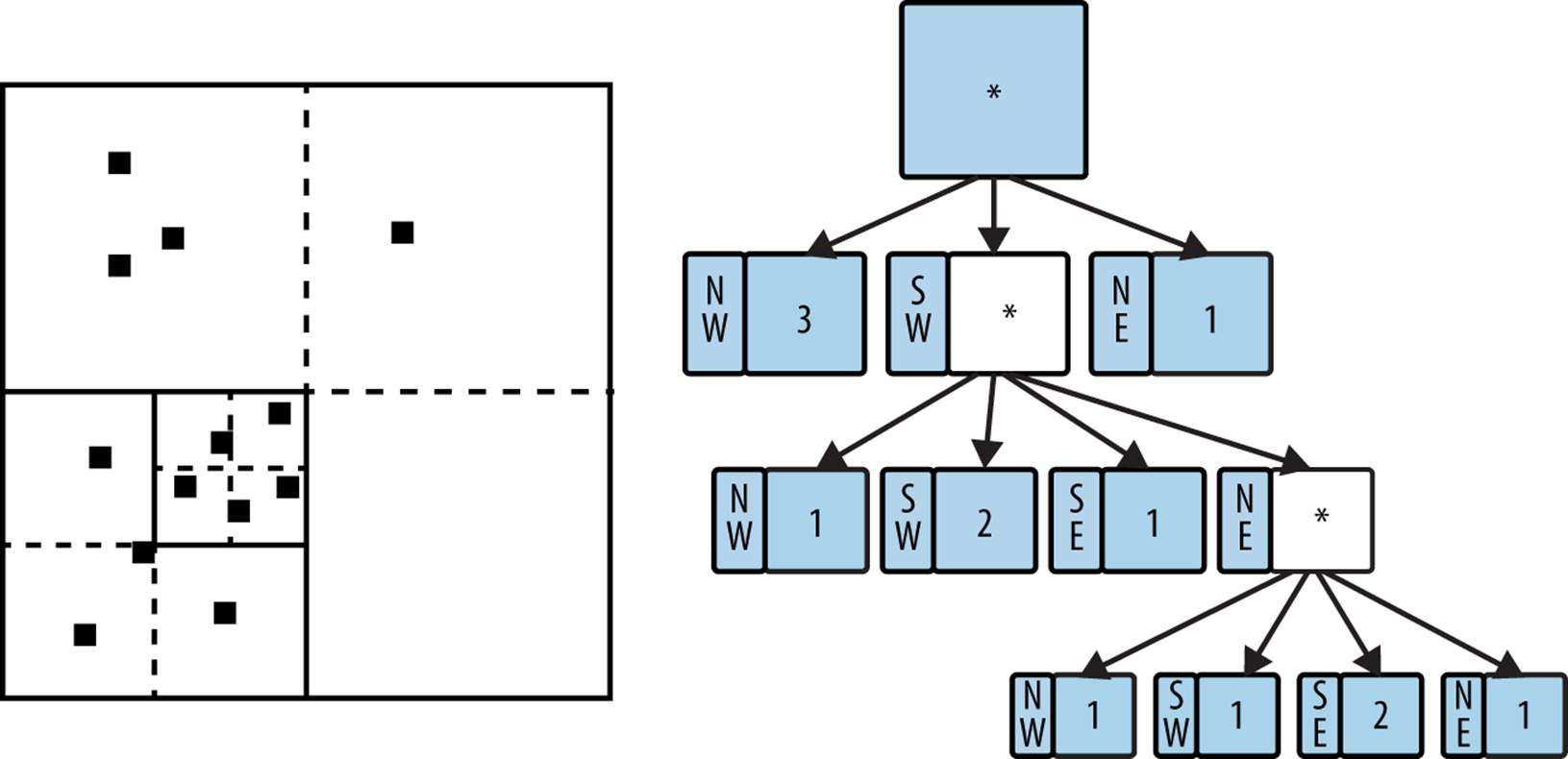
Figure 10-4. Quadtree using point-based partitioning

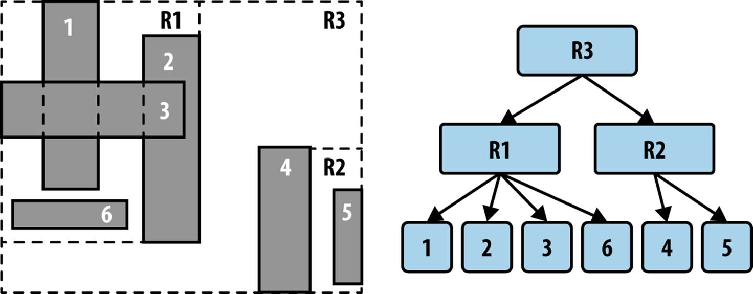
Figure 10-5. R-Tree example

The root node represents the smallest rectangular region (x_low, y_low, x_high, y_high) that includes all other rectangles in the tree. Each interior node has an associated rectangular region that similarly includes all rectangles in its descendant nodes. The actual rectangles in the R-Tree are stored only in leaf nodes. Aside from the root node, every rectangular region (whether associated with an interior node or a leaf node) is wholly contained by the region of its parent node.

We now use these various spatial structures to solve the problems outlined at the beginning of this chapter.

Nearest Neighbor Queries

Given a set of two-dimensional points, P, you are asked to determine which point in P is closest to a target query point, x. We show how to use k-d trees to efficiently perform these queries. Assuming the tree is effective in partitioning the points, each recursive traversal through the tree will discard roughly half of the points in the tree. In a k-d tree for points distributed in a normal manner, nodes on level i reflect rectangles that are roughly twice as large as the rectangles on level i + 1. This property will enable Nearest Neighbor to exhibit O(log n) performance because it will be able to discard entire subtrees containing points that are demonstrably too far to be the closest point. However, the recursion is a bit more complex than for regular binary search trees, as we will show.

As shown in Figure 10-6, if the target point (shown as a small black square) were inserted, it would become a child of the node associated with point 9. Upon calling nearest with this selection, the algorithm can discard the entire left subtree because the perpendicular distance dp is not closer, so none of those points can be closer. Recursing into the right subtree, the algorithm detects that point 3 is closer. Further, it determines that the perpendicular distance to point 3 is closer than min so it must recursively investigate both subtrees rooted at points 7 and 8. Ultimately it determines that point 3 is the closest point.

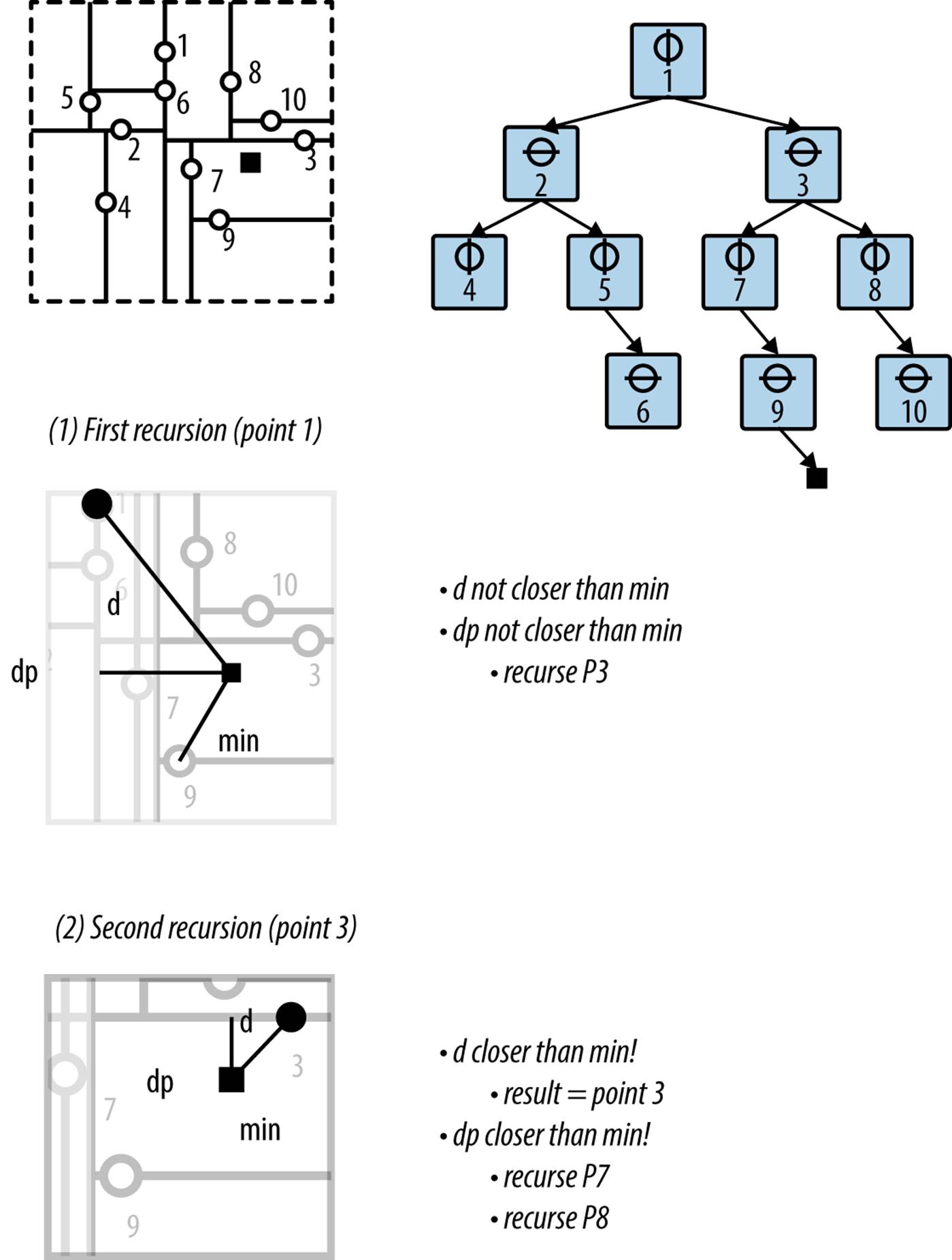
Figure 10-6. Nearest Neighbor example

NEAREST NEIGHBOR SUMMARY

Best, Average: O(log n) Worst: O(n)

nearest (T, x)

n = find parent node in T where x would have been inserted

min = distance from x to n.point

better = nearest (T.root, min, x)

if better found then return better

return n.point

end

nearest (node, min, x)

d = distance from x to node.point

if d < min then

result = node.point

min = d

dp = perpendicular distance from x to node

if dp < min then

pt = nearest (node.above, min, x)

if distance from pt to x < min then

result = pt

min = distance from pt to x

pt = nearest (node.below, min, x)

if distance from pt to x < min then

result = pt

min = distance from pt to x

else

if node is above x then

pt = nearest (node.above, min, x)

else

pt = nearest (node.below, min, x)

if pt exists then return pt

return result

end

Choose reasonable best guess for closest point.

Traverse again from root to try to find better one.

A closer point is found.

If too close to call, check both above and below subtrees.

Otherwise, can safely check only one subtree.

Input/Output

The input is a k-d tree formed from a set of two-dimensional points P in a plane. A set of nearest neighbor queries (not known in advance) is issued one at a time to find the nearest point in P to a point x.

For each query point x, the algorithm computes a point in P that is the closest neighbor to x.

If two points are “too close” to each other through floating-point error, the algorithm may incorrectly select the wrong point; however, the distance to the actual closest point would be so close that there should be no impact by this faulty response.

Context

When comparing this approach against a brute-force approach that compares the distances between query point x and each point p ∈ P, there are two important costs to consider: (1) the cost of constructing the k-d tree, and (2) the cost of locating the query point x within the tree structure. The trade-offs that impact these costs are:

Number of dimensions

As the number of dimensions increases, the cost of constructing the k-d tree overwhelms its utility. Some authorities believe that for more than 20 dimensions, this approach is less efficient than a straight comparison against all points.

Number of points in the input set

When the number of points is small, the cost of constructing the structure may outweigh the improved performance.

Binary trees can be efficient search structures because they can be balanced as nodes are inserted into and deleted from the tree. Unfortunately, k-d trees cannot be balanced easily, nor can points be deleted, because of the deep structural information about the dimensional plane they represent. The ideal solution is to construct the initial k-d tree so that either (a) the leaf nodes are at the same level in the tree, or (b) all leaf nodes are within one level of all other leaf nodes.

Solution

Given an existing k-d tree, Nearest Neighbor implementation is shown in Example 10-1.

Example 10-1. Nearest Neighbor implementation in KDTree

// KDTree method.

public IMultiPoint nearest (IMultiPoint target) {

if (root == null||target == null) return null;

// Find parent node to which target would have been inserted.

// Best shot at finding closest point.

DimensionalNode parent = parent (target);

IMultiPoint result = parent.point;

double smallest = target.distance (result);

// Start back at the root to try to find closer one.

double best[] = new double[] { smallest };

double raw[] = target.raw();

IMultiPoint betterOne = root.nearest (raw, best);

if (betterOne != null) { return betterOne; }

return result;

}

// DimensionalNode method. min[0] is best computed shortest distance.

IMultiPoint nearest (double[] rawTarget, double min[]) {

// Update minimum if we are closer.

IMultiPoint result = null;

// If shorter, update minimum

double d = shorter (rawTarget, min[0]);

if (d >= 0 && d < min[0]) {

min[0] = d;

result = point;

}

// determine if we must dive into the subtrees by computing direct

// perpendicular distance to the axis along which node separates

// the plane. If d is smaller than the current smallest distance,

// we could "bleed" over the plane so we must check both.

double dp = Math.abs (coord — rawTarget[dimension-1]);

IMultiPoint newResult = null;

if (dp < min[0]) {

// must dive into both. Return closest one.

if (above != null) {

newResult = above.nearest (rawTarget, min);

if (newResult != null) { result = newResult; }

}

if (below != null) {

newResult = below.nearest (rawTarget, min);

if (newResult != null) { result = newResult; }

}

} else {

// only need to go in one! Determine which one now.

if (rawTarget[dimension-1] < coord) {

if (below != null) {

newResult = below.nearest (rawTarget, min);

}

} else {

if (above != null) {

newResult = above.nearest (rawTarget, min);

}

}

// Use smaller result, if found.

if (newResult != null) { return newResult; }

}

return result;

}

The key to understanding Nearest Neighbor is that we first locate the region where the target point would have been inserted, since this will likely contain the closest point. We then validate this assumption by recursively checking from the root back down to this region to see whether some other point is actually closer. This could easily happen because the rectangular regions of the k-d tree were created based on the set of input points. In unbalanced k-d trees, this checking process might incur an O(n) total cost, reinforcing the notion that the input set must be properly processed.

The example solution has two improvements to speed up its performance. First, the comparisons are made on the “raw” double array representing each point. Second, a shorter method in DimensionalNode is used to determine when the distance between two d-dimensional points is smaller than the minimum distance computed so far; this method exits immediately when a partial computation of the Euclidean distance exceeds the minimum found.

Assuming the initial k-d tree is balanced, the search can advantageously discard up to half of the points in the tree during the recursive invocations. Two recursive invocations are sometimes required, but only when the computed minimum distance is just large enough to cross over the dividing line for a node, in which case both sides need to be explored to find the closest point.

Analysis

The k-d tree is initially constructed as a balanced k-d tree, where the dividing line on each level is derived from the median of the points remaining at that level. Locating the parent node of the target query can be found in O(log n) by traversing the k-d tree as if the point were to be inserted. However, the algorithm may make two recursive invocations: one for the child above and one for the child below.

If the double recursion occurs frequently, the algorithm degrades to O(n), so it is worth understanding how often it can occur. The multiple invocations occur only when the perpendicular distance, dp, from the target point to the node’s point is less than the best computed minimum. As the number of dimensions increases, there are more potential points that satisfy these criteria.

Table 10-1 provides some empirical evidence to show how often this occurs. A balanced k-d tree is created from n = 4 to 131,072 random two-dimensional points generated within the unit square. A set of 50 nearest point queries is issued for a random point within the unit square, andTable 10-1 records the average number of times two recursive invocations occurred (i.e., when dp < min[0] and the node in question has children both above and below), as compared to single recursive invocations.

From this random data, the number of double recursions appears to be .3*log(n) for two dimensions, but this jumps to 342*log(n) for 10 dimensions (a 1,000-fold increase). The important observation is that both of these estimation functions conform to O(log n).

But what happens when d increases to be “sufficiently close” to n in some way? The data graphed in Figure 10-7 shows that as d increases, the number of double recursions actually approaches n/2. In fact, as d increases, the number of single recursions conforms to a normal distribution whose mean is very close to log(n), which tells us that eventually all recursive invocations are of the double variety. The impact this discovery has on the performance of nearest-neighbor queries is that as d approaches log(n), the investment in using k-d trees begins to diminish until the resulting performance is no better than O(n), because the number of double recursions plateaus at n/2.

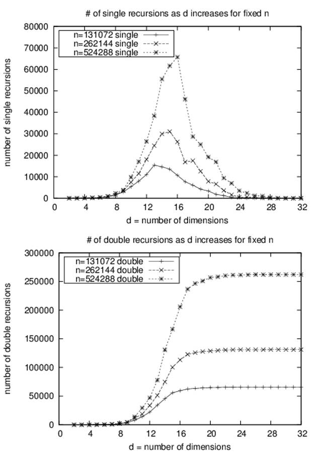
Figure 10-7. Number of double recursions as n and d increase

Certain input set data sets force Nearest Neighbor to work hard even in two dimensions. For example, let’s change the input for Table 10-1 such that the n unique two-dimensional points are found on the edge of a circle of radius r > 1, but the nearest query points still lie within the unit square. When n = 131,072 points, the number of single recursions has jumped 10-fold to 235.8 while the number of double recursions has exploded to 932.78 (a 200-fold increase!). Thus, the nearest neighbor query will degenerate in the worst case to O(n) given specifically tailored queries for a given input set. Figure 10-8 demonstrates a degenerate k-d tree with 64 points arranged in a circle.

We can also evaluate the performance of k-d tree Nearest Neighbor against a straight brute-force O(n) comparison. Given a data set of size n = 131,072 points, where 128 searches random are to be executed, how large must the dimensionality d of the input set be before the brute-forceNearest Neighbor implementation outperforms the k-d tree implementation?

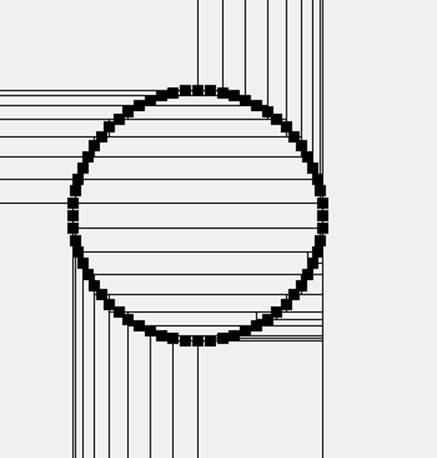
Figure 10-8. Circular data set leads to inefficient k-d tree

We ran 100 trials and discarded the best and worst trials, computing the average of the remaining 98 trials. The results are graphed in Figure 10-9 and show that for d = 11 dimensions and higher, the brute-force nearest neighbor implementation outperforms the Nearest Neighbor k-d tree algorithm. The specific crossover point depends on the machine hardware on which the code executes, the specific values of n and d, and the distribution of points in the input set. We do not include in this crossover analysis the cost of constructing the k-d tree, because that cost can be amortized across all searches.

The results in Figure 10-9 confirm that as the number of dimensions increases, the benefit of using Nearest Neighbor over brute force decreases. The cost of constructing the k-d trees is not a driving factor in the equation, because that is driven primarily by the number of data points to be inserted into the k-d tree, not by the number of dimensions. On larger data set sizes, the savings is more pronounced. Another reason for the worsening performance as d increases is that computing the Euclidean distance between two d-dimensional points is an O(d) operation. Although it can still be considered a constant time operation, it simply takes more time.

To maximize the performance of k-d tree searches, the tree must be balanced. Example 10-2 demonstrates the well-known technique for constructing a balanced k-d tree using recursion to iterate over each of the coordinate dimensions. Simply put, it selects the median element from a set of points to represent the node; the elements below the median are inserted into the below subtree, whereas elements above the median are inserted into the above subtree. The code works for arbitrary dimensions.

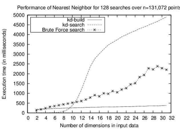
Figure 10-9. Comparing k-d tree versus brute-force implementation

Example 10-2. Recursively construct a balanced k-d tree

public class KDFactory {

private static Comparator<IMultiPoint> comparators[];

// Recursively construct KDTree using median method on points.

public static KDTree generate (IMultiPoint []points) {

if (points.length == 0) { return null; }

// median will be the root.

int maxD = points[0].dimensionality();

KDTree tree = new KDTree(maxD);

// Make dimensional comparators that compare points by ith dimension

comparators = new Comparator[maxD+1];

for (int i = 1; i <= maxD; i++) {

comparators[i] = new DimensionalComparator(i);

}

tree.setRoot (generate (1, maxD, points, 0, points.length-1));

return tree;

}

// generate node for d-th dimension (1 <= d <= maxD)

// for points[left, right]

private static DimensionalNode generate (int d, int maxD,

IMultiPoint points[],

int left, int right) {

// Handle the easy cases first

if (right < left) { return null; }

if (right == left) { return new DimensionalNode (d, points[left]); }

// Order the array[left,right] so mth element will be median and

// elements prior to it will be <= median, though not sorted;

// similarly, elements after will be >= median, though not sorted

int m = 1+(right-left)/2;

Selection.select (points, m, left, right, comparators[d]);

// Median point on this dimension becomes the parent

DimensionalNode dm = new DimensionalNode (d, points[left+m-1]);

// update to the next dimension, or reset back to 1

if (++d > maxD) { d = 1; }

// recursively compute left and right subtrees, which translate

// into 'below' and 'above' for n-dimensions.

dm.setBelow (maxD, generate (d, maxD, points, left, left+m-2));

dm.setAbove (maxD, generate (d, maxD, points, left+m, right));

return dm;

}

}

The select operation was described in Chapter 4. It can select the k^th smallest number recursively in O(n) time in the average case; however, it does degrade to O(n²) in the worst case.

Variations

In the implementation we have shown, the method nearest traverses from the root back down to the computed parent; alternate implementations start from the parent and traverse back to the root, in bottom-up fashion.

Range Query

Given a rectangular range R defined by (x_low, y_low, x_high, y_high) and a set of points P, which points in P are contained within a target rectangle T? A brute-force algorithm that inspects all points in P can determine the enclosed points in O(n)—can we do better?

For Nearest Neighbor, we organized the points into a k-d tree to process nearest-neighbor queries in O(log n) time. Using the same data structure, we now show how to compute Range Query in O(n^0.5 + r), where r is the number of points reported by the query. Indeed, when the input set contains d-dimensional data points, the solution scales to solve d-dimensional Range Query problems in O(n^1–1/d + r).

Given target region, T, which covers the left half of the plane to just beyond point 7 in Figure 10-10, we can observe all three of these cases. Since T does not wholly contain the infinite region associated with the root node, Range Query checks whether T contains point 1, which it does, so that point is added to the result. Now T extends into both its above and below children, so both recursive calls are made. In the first recursion below point 1, T wholly contains the region associated with point 2. Thus, point 2 and all of its descendants are added to the result. In the second recursion, eventually point 7 is discovered and added to the result.

RANGE QUERY SUMMARY

Best, Average: O(n^1-1/d + r) Worst: O(n)

range (space)

results = new Set

range (space, root, results)

return results

end

range (space, node, results)

if space contains node.region then

add node.points andall of its descendants to results

return

if space contains node.point then

add node.point to results

if space extends below node.coord then

range (space, node.below, results)

if space extends above node.coord then

range (space, node.above, results)

end

Should a k-d tree node be wholly contained by search space, all descendants are added to results.

Ensure point is added to results if contained.

May have to search both above and below.

Input/Output

The input is a set of n points P in d-dimensional space and a d-dimensional hypercube that specifies the desired range query. The range queries are aligned properly with the axes in the d-dimensional data set because they are specified by d individual ranges, for each dimension of the input set. For d = 2, the range query has both a range over x coordinates and a range over y coordinates.

Range Query generates the full set of points enclosed by the range query. The points do not appear in any specific order.

Context

k-d trees become unwieldy for a large number of dimensions, so this algorithm and overall approach should be restricted to small dimensional data. For two-dimensional data, k-d trees offers excellent performance for Nearest Neighbor and Range Query problems.

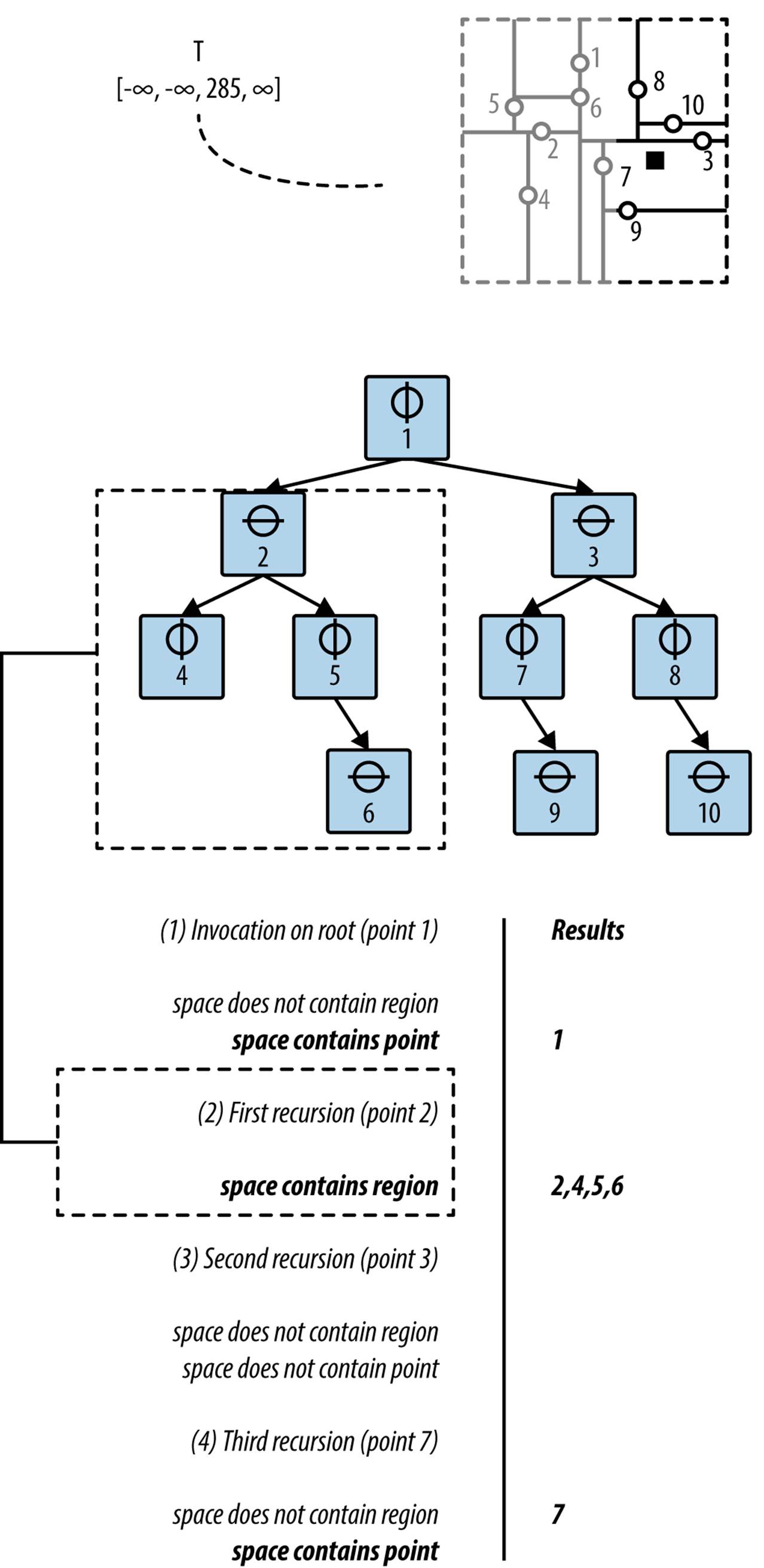
Figure 10-10. Range Query example

Solution

The Java solution shown in Example 10-3 is a method of the DimensionalNode class, which is simply delegated by the range(IHypercube) method found in KDTree. The key efficiency gain of this algorithm occurs when the region for a DimensionalNode is wholly contained within the desired range query. In this circumstance, all descendant nodes of the DimensionalNode can be added to the results collection because of the k-d tree property that the children for a node are wholly contained within the region of any of its ancestor nodes.

Example 10-3. Range Query implementation in DimensionalNode

public void range (IHypercube space, KDSearchResults results) {

// Wholly contained? Take all descendant points

if (space.contains (region)) {

results.add (this);

return;

}

// Is our point at least contained?

if (space.intersects (cached)) {

results.add (point);

}

// Recursively progress along both ancestral trees, if demanded.

// The cost in manipulating space to be "cropped" to the proper

// structure is excessive, so leave alone and is still correct.

if (space.getLeft(dimension) < coord) {

if (below != null) { below.range (space, results); }

}

if (coord < space.getRight(dimension)) {

if (above != null) { above.range (space, results); }

}

}

The code shown in Example 10-3 is a modified tree traversal that potentially visits every node in the tree. Because the k-d tree partitions the d-dimensional data set in hierarchical fashion, there are three decisions Range Query makes at each node n:

Is the region associated with node n fully contained within the query region?

When this happens, the range traversal can stop because all descendant points belong to the query result.

Does the query region contain the point associated with node n?

If so, add the point associated with n to the result set.

Along the dimension d represented by node n, does query region intersect n?

It can do so in two ways since the query region can intersect both the region associated with n’s below subtree as well as the region associated with n’s above subtree. The code may perform zero, one, or two recursive traversals of range.

Observe that the result returned is a KDSearchResults object that contains both individual points as well as entire subtrees. Thus, to retrieve all points you will have to traverse each subtree in the result.

Analysis

It is possible that the query region contains all points in the tree, in which case all points are returned, which leads to O(n) performance. However, when Range Query detects that the query region does not intersect an individual node within the k-d tree, it can prune the traversal. The cost savings depend on the number of dimensions and the specific nature of the input set. Preparata and Shamos (1985) showed that Range Query using k-d trees performs in O(n^1–1/d + r), where r is the number of results found. As the number of dimensions increases, the benefit decreases.

Figure 10-11 graphs the expected performance of an O(n^1–1/d) algorithm; the distinctive feature of the graph is fast performance for small values of d that over time inexorably approaches O(n). Because of the addition of r (the number of points returned by the query), the actual performance will deviate from the ideal curve shown in Figure 10-11.

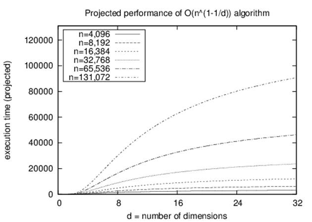
Figure 10-11. Expected performance for O(n^1-1/d) algorithm

It is difficult to produce sample data sets to show the performance of Range Query. We demonstrate the effectiveness of Range Query on a k-d tree by comparing its performance to a brute-force implementation that inspects each point against the desired query region. The d-dimensional input set for each of these situations contains n points whose coordinate values are drawn uniformly from the range [0, s], where s = 4,096. We evaluate three situations:

Query region contains all points in the tree

We construct a query region that contains all of the points in the k-d tree. This example provides the maximum speed-up supported by the algorithm; its performance is independent of the number of dimensions d in the k-d tree. The k-d tree approach takes about 5–7 times as long to complete; this represents the overhead inherent in the structure. In Table 10-2, the performance cost for the brute-force region query increases as d increases because computing whether a d-dimensional point is within a d-dimensional space is an O(d) operation, not constant. The brute-force implementation handily outperforms the k-d tree implementation.

Fractional regions

Because the number of results found, r, plays a prominent role in determining the performance of the algorithm, we construct a set of scenarios to isolate this variable as the number of dimensions increases.

The uniformity of the input set discourages us from simply constructing a query region [.5*s, s] for each dimension of input. If we did this, the total volume of the input set queried is (1/2)^d, which implies that as d increases the number of expected points, r, returned by the query region decreases. Instead, we construct query regions whose size increases as d increases. For example, in two dimensions the query region with [.5204*s, s] on each dimension should return .23*n points because (1 – .5204)² = .23. However, for three dimensions the query region must expand to [.3873*s, s] on each dimension since (1 – .3873)³ = .23.

Using this approach, we fix in advance the desired ratio k such that our constructed query will return k*n points (where k is either 0.23, 0.115, 0.0575, 0.02875, or 0.014375). We compare the k-d tree implementation against a brute-force implementation as n varies from 4,096 to 131,072 and d varies from 2 to 15, as shown in Figure 10-12. The charts on the left side show the distinctive behavior of the O(n^1–1/d) k-d tree algorithm while the right side shows the linear performance of brute force. For a 0.23 ratio, the k-d tree implementation outperforms brute force only for d= 2 and n ≤ 8,192; however, for a ratio of 0.014375, the k-d tree implementation wins for d ≤ 6 and n ≤ 131,072.

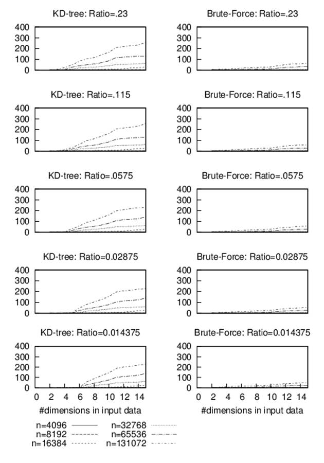
Figure 10-12. Comparing k-d tree versus brute force for fractional regions

Empty region

We construct a query region from a single random point drawn uniformly from the same values for the input set. Performance results are shown in Table 10-3. The k-d tree executes nearly instantaneously; all recorded execution times are less than a fraction of a millisecond.

Quadtrees

Quadtrees can be used to solve the following queries:

Range queries

Given a collection of points in the Cartesian plane, determine the points that exist within a query rectangle. A sample application is shown in Figure 10-13 where a dashed rectangle is selected by the user, and points contained within the rectangle are highlighted. When a quadtree region is wholly contained by the target query, the application draws that region with a shaded background.

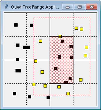
Figure 10-13. Range searching using a quadtree

Collision detection

Given a collection of objects in the Cartesian plane, determine all intersections among the objects. A sample application is shown in Figure 10-14 that identifies the collisions among a number of moving squares that bounce back and forth within a window. Squares that intersect each other are highlighted.

QUADTREE SUMMARY

Best, Average, Worst: O(log n)

add (node, pt)

if node.region does notcontain pt then

return false

if node is leaf node then

if node already contains pt then

return false

if node has < 4 points then

add pt to node

return true

q = quadrant for pt in node

if node is leaf node then

node.subdivide()

return add(node.children[q], pt)

range (node, rect, result)

if rect contains node.region then

add (node, true) to result

else if node is leaf node then

foreach point p in node do

if rect contains p then

add (p, false) to result

else

foreach child in node.children do

if rect overlaps child.region

range(child, rect, result)

Impose set semantics on quadtree.

Each node can store up to four points.

Leaf points are distributed among four new children.

Insert new point into correct child.

Entire subtree is contained and returned.

Individual points returned.

Recursively check each overlapping child.

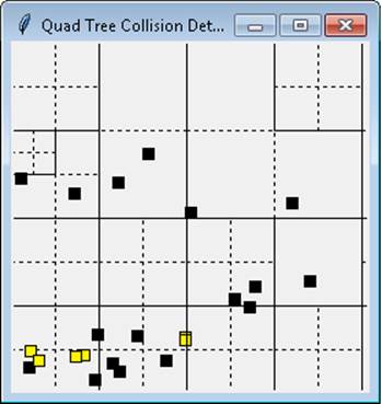
Figure 10-14. Collision detection using a quadtree

Input/Output

The input is a set of two-dimensional points P in a plane from which a quadtree is constructed.

For optimal performance, a range query returns the nodes in the quadtree, which allows it to return entire subtrees of points when the target rectangle wholly contains a subtree of points. The results of a collision detection are the existing points that intersect with a target point.

Solution

The basis of the Python implementation of quadtree is the QuadTree and QuadNode structures shown in Example 10-4. The smaller2k and larger2k helper methods ensure the initial region has sides that are powers of two. The Region class represents a rectangular region.

Example 10-4. Quadtree QuadNode implementation

class Region:

def __init__(self, xmin,ymin, xmax,ymax):

"""

Creates region from two points (xmin,ymin) to (xmax,ymax). Adjusts if

these are not the bottom-left and top-right coordinates for a region.

"""

self.x_min = xmin if xmin < xmax else xmax

self.y_min = ymin if ymin < ymax else ymax

self.x_max = xmax if xmax > xmin else xmin

self.y_max = ymax if ymax > ymin else ymin

class QuadNode:

def __init__(self, region, pt = None, data = None):

"""Create empty QuadNode centered on origin of given region."""

self.region = region

self.origin = (region.x_min + (region.x_max - region.x_min)//2,

region.y_min + (region.y_max - region.y_min)//2)

self.children = [None] * 4

if pt:

self.points = [pt]

self.data = [data]

else:

self.points = []

self.data = []

class QuadTree:

def __init__(self, region):

"""Create QuadTree over square region whose sides are powers of 2."""

self.root = None

self.region = region.copy()

xmin2k = smaller2k(self.region.x_min)

ymin2k = smaller2k(self.region.y_min)

xmax2k = larger2k(self.region.x_max)

ymax2k = larger2k(self.region.y_max)

self.region.x_min = self.region.y_min = min(xmin2k, ymin2k)

self.region.x_max = self.region.y_max = max(xmax2k, ymax2k)

Points are added to the quadtree using the add method shown in Example 10-5. The add method returns False if the point is already contained within the quadtree, thus it enforces mathematical set semantics. Up to four points are added to a node if the point is contained within that node’s rectangular region. When the fifth point is added, the node’s region is subdivided into quadrants and the points are reassigned to the individual quadrants of that node’s region; should all points be assigned to the same quadrant, the process repeats until all leaf quadrants have four or fewer points.

Example 10-5. Quadtree add implementation

class QuadNode:

def add (self, pt, data):

"""Add (pt, data) to the QuadNode."""

node = self

while node:

# Not able to fit in this region.

if notcontainsPoint (node.region, pt):

return False

# if we have points, then we are leaf node. Check here.

if node.points != None:

if pt innode.points:

return False

# Add if room

if len(node.points) < 4:

node.points.append (pt)

node.data.append (data)

return True

# Find quadrant into which to add.

q = node.quadrant (pt)

if node.children[q] isNone:

# subdivide and reassign points to each quadrant. Then add point.

node.subdivide()

node = node.children[q]

return False

class QuadTree:

def add (self, pt, data = None):

if self.root isNone:

self.root = QuadNode(self.region, pt, data)

return True

return self.root.add (pt, data)

With this structure, the range method in Example 10-6 demonstrates how to efficiently locate all points in the quadtree that are contained by a target region. This Python implementation uses the yield operator to provide an iterator interface to the results. The iterator contains tuples that are either individual points or entire nodes. When a quadtree node is wholly contained by a region, that entire node is returned as part of the result. The caller can retrieve all descendant values using a preorder traversal of the node, provided by QuadNode.

Example 10-6. Quadtree Range Query implementation

class QuadNode:

def range(self, region):

"""

Yield (node,True) when node contained within region,

otherwise (region,False) for individual points.

"""

if region.containsRegion (self.region):

yield (self, True)

else:

# if we have points, then we are leaf node. Check here.

if self.points != None:

for i inrange(len(self.points)):

if containsPoint (region, self.points[i]):

yield ((self.points[i], self.data[i]), False)

else:

for child inself.children:

if child.region.overlap (region):

for pair inchild.range (region):

yield pair

class QuadTree:

def range(self, region):

"""Yield (node,status) in Quad Tree contained within region."""

if self.root isNone:

return None

return self.root.range(region)

To support collision detection, Example 10-7 contains the collide method which searches through the quadtree to locate points in the tree that intersect a square with sides of length r centered at a given point, pt.

Example 10-7. Quadtree collision detection implementation

class QuadNode:

def collide (self, pt, r):

"""Yield points in leaf that intersect with pt and square side r."""

node = self

while node:

# Point must fit in this region

if containsPoint (node.region, pt):

# if we have points, then we are leaf node. Check here

if node.points != None:

for p,d inzip(node.points, node.data):

if p[X]-r <= pt[X] <= p[X]+r andp[Y]-r <= pt[Y] <= p[Y]+r:

yield (p, d)

# Find quadrant into which to check further

q = node.quadrant (pt)

node = node.children[q]

class QuadTree:

def collide(self, pt, r):

"""Return collisions to point within Quad Tree."""

if self.root isNone:

return None

return self.root.collide (pt, r)

Analysis

Quadtrees partition the points in a plane using the same underlying structure of binary search trees. The region-based implementation presented here uses a fixed partitioning scheme that leads to efficient behavior when the collection of points is uniformly distributed. It may happen that the points are all clustered together in a small space, as shown in Figure 10-15. Thus, the search performance is logarithmic with respect to the tree size. The range query in Python is made efficient by returning both individual points as well as entire nodes in the quadtree; however, you must still consider the time to extract all descendant values in the nodes returned by the range query.

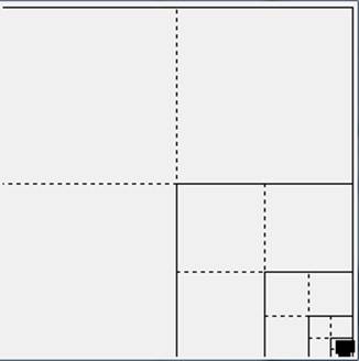
Figure 10-15. Degenerate quadtree

Variations

The quadtree structure presented here is a region quadtree. A point quadtree represents two-dimensional points. The Octree extends quadtree into three dimensions, with eight children (as with a cube) instead of four (Meagher, 1995).

R-Trees

Balanced binary trees are an incredibly versatile data structure that offer great performance for search, insert, and delete operations. However, they work best in primary memory using pointers and allocating (and releasing) nodes as needed. These trees can only grow as large as primary memory and they are not easily stored to secondary storage, such as a file system. Operating systems provide virtual memory so programs can operate using an assigned memory space, which might be larger than the actual memory. The operating system ensures a fixed-size block of memory (known as a page) is brought into primary memory as needed, and older unused pages are stored to disk (if modified) and discarded. Programs work most efficiently when consolidating read and write access using pages, which are typically 4,096 bytes in size. If you consider that a node in a binary tree might only require 24 bytes of storage, there would be dozens of such nodes packed to a page. It is not immediately clear how to store these binary nodes to disk especially when the tree is dynamically updated.

The B-Tree concept was developed by Bayer and McCreight in 1972, though it appears to have been independently discovered by vendors of database management systems and operating systems. A B-Tree extends the structure of a binary tree by allowing each node to store multiple values and multiple links to more than two nodes. A sample B-Tree is shown in Figure 10-16.

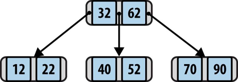
Figure 10-16. Sample B-Tree

Each node n contains a number of ascending values { k₁, k₂, …, k_m–1 } and pointers { p₁, p₂, …, p_m } where m determines the maximum number of children nodes that n can point to. The value m is known as the order of the B-Tree. Each B-Tree node can contain m-1 values.

To maintain the binary search tree property, B-Tree nodes store key values such that all values in the subtree pointed to by p₁ are smaller than k₁. All values in the subtree pointed to by p_i are greater than or equal to k_i and smaller than k_i+1. Finally, all values in the subtree pointed to by p_m are greater than k_m–1.

Using Knuth’s definition, a B-Tree of order m satisfies the following:

§ Every node has at most m children.

§ Every nonleaf node (except the root) has at least ⌈m ⁄ 2⌉ children.

§ The root has at least two children if it is not a leaf node.

§ A nonleaf node with k children nodes contains k − 1 key values.

§ All leaves appear in the same level.

Using this definition, a traditional binary tree is a degenerate B-Tree of order m = 2. Insertions and deletions in a B-Tree must maintain these properties. In doing so, the longest path in a B-Tree with n keys contains at most log_m(n) nodes, leading to O(log n) performance for its operations. B-Trees can be readily stored to secondary storage by increasing the number of keys in each node so that its total size properly aligns with the page size (e.g., storing two B-Tree nodes per page), which minimizes the number of disk reads to load nodes into primary memory.

With this brief sketch of B-Trees, we can now describe in more detail the R-Tree structure. An R-Tree is a height-balanced tree, similar to a B-Tree, that stores n-dimensional spatial objects in a dynamic structure that supports insert, delete, and query operations. It also supports range queriesfor locating objects that overlap with a target n-dimensional query. In this chapter, we describe the fundamental operations that maintain R-Trees to ensure efficient execution of the core operations.

An R-Tree is a tree structure in which each node contains links to up to M different children nodes. All information is stored by the leaf nodes, each of which can store up to M different n-dimensional spatial objects. An R-Tree leaf node provides an index into the actual repository that stores the objects themselves; the R-Tree only stores the unique identifier for each object and the n-dimensional bounding box, I, which is the smallest n-dimensional shape that contains the spatial object. In this presentation we assume two dimensions and these shapes are rectangles, but it can naturally be extended to n dimensions based on the structure of the data.

There is another relevant constant, m ≤ ⌊M/2⌋, which defines the minimum number of values stored by a leaf node or links stored by interior nodes in the R-Tree. We summarize the R-Tree properties here:

§ Every leaf node contains between m and M (inclusive) records [unless it is the root].

§ Every nonleaf node contains between m and M (inclusive) links to children nodes [unless it is the root].

§ For each entry (I, child_i) in a nonleaf node, I is the smallest rectangle that spatially contains the rectangles in its children nodes.

§ The root node has at least two children [unless it is a leaf].

§ All leaves appear on the same level.

The R-Tree is a balanced structure that ensures the properties just listed. For convenience, the leaf level is considered level 0, and the level number of the root node is the height of the tree. The R-Tree structure supports insertion, deletion, and query in O(log_m n).

The repository contains sample applications for investigating the behavior of R-Trees. Figure 10-17 shows the dynamic behavior as a new rectangle 6 is added to the R-Tree that contains M = 4 shapes. As you can see, there is no room for the new rectangle, so the relevant leaf node R1 is splitinto two nodes, based on a metric that seeks to minimize the area of the respective new nonleaf node, R2. Adding this rectangle increases the overall height of the R-Tree by one since it creates a new root, R3.

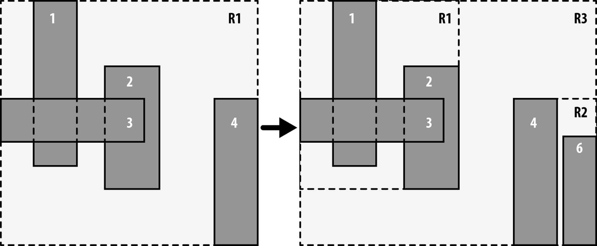
Figure 10-17. R-Tree insert example

R-TREE SUMMARY

Best, Average: O(log_m n) Worst: O(n)

add (R, rect)

if R is empty then

R = new RTree (rect)

else

leaf = chooseLeaf(rect)

if leaf.count < M then

add rect to leaf

else

newLeaf = leaf.split(rect)

newNode = adjustTree (leaf, newLeaf)

if newNode != null then

R = new RTree with old Root andnewNode as children

end

search (n, t)

if n is a leaf then

return entry if n contains t otherwise False

else

foreach child c of n do

if c contains t then

return search(c, t)

end

range (n, t)

if target wholly contains n's bounding box then

return all descendant rectangles

else if n is a leaf

return all entries that intersect t

else

result = null

foreach child c of n do

if c overlaps t then

result = union of result andrange(c, t)

return result

Entries are added to a leaf node if there is room.

Otherwise, M + 1 entries are divided among the old leaf and a new node.

Entries in path to root may need to be adjusted.

R-Tree might grow in height after an add.

Leaf nodes contain the actual entries.

Recursively search each child since regions may overlap.

Once found the entry is returned.

Efficient operation for detecting membership.

May have to execute multiple recursive queries.

Input/Output

A two-dimensional R-Tree stores a collection of rectangular regions in the Cartesian plane, each with its own (optional) unique identifier.

R-Tree operations can modify the state of the R-Tree (i.e., insert or delete) as well as retrieve an individual rectangular region or a collection of regions.

Context

R-Trees were designed to index multidimensional information including geographical structures or more abstract n-dimensional data, such as rectangles or polygons. This is one of the few structures that offers excellent runtime performance even when the information is too large to store in main memory. Traditional indexing techniques are inherently one-dimensional and thus R-Tree structures are well-suited for these domains.

The operations on an R-Tree include insertion and deletion, and there are two kinds of queries. You can search for a specific rectangular region in the R-Tree or you can determine the collection of rectangular regions that intersect a query rectangle.

Solution

The Python implementation in Example 10-8 associates an optional identifier with each rectangle; this would be used to retrieve the actual spatial object from the database. We start with the RNode, which is the fundamental unit of an R-Tree. Each RNode maintains a bounding region and an optional identifier. An RNode is a leaf if node.level is zero. There are node.count children for an RNode and they are stored in the node.children list. When adding a child RNode, the parent node.region bounding box must be adjusted to include the newly added child.

Example 10-8. RNode implementation

class RNode:

# Monotonically incrementing counter to generate identifiers

counter = 0

def __init__(self, M, rectangle = None, ident = None, level = 0):

if rectangle:

self.region = rectangle.copy()

else:

self.region = None

if ident isNone:

RNode.counter += 1

self.id = 'R' + str(RNode.counter)

else:

self.id = ident

self.children = [None] * M

self.level = level

self.count = 0

def addRNode(self, rNode):

"""Add previously computed RNode and adjust bounding region."""

self.children[self.count] = rNode

self.count += 1

if self.region isNone:

self.region = rNode.region.copy()

else:

rectangle = rNode.region

if rectangle.x_min < self.region.x_min:

self.region.x_min = rectangle.x_min

if rectangle.x_max > self.region.x_max:

self.region.x_max = rectangle.x_max

if rectangle.y_min < self.region.y_min:

self.region.y_min = rectangle.y_min

if rectangle.y_max > self.region.y_max:

self.region.y_max = rectangle.y_max

With this base in place, Example 10-9 describes the RTree class and the method for adding a rectangle to an R-Tree.

Example 10-9. RTree and corresponding add implementation

class RTree:

def __init__(self, m=2, M=4):

"""Create empty R tree with (m=2, M=4) default values."""

self.root = None

self.m = m

self.M = M

def add(self, rectangle, ident = None):

"""Insert rectangle into proper location with (optional) identifier."""

if self.root isNone:

self.root = RNode(self.M, rectangle, None)

self.root.addEntry (self.M, rectangle, ident)

else:

# I1 [Find position for new record] Invoke ChooseLeaf to select

# a leaf node L in which to place E. Path to leaf returned.

path = self.root.chooseLeaf (rectangle, [self.root]);

n = path[-1]

del path[-1]

# I2 [Add record to leaf node] If L has room for another entry,

# install E. Otherwise invoke SplitNode to obtain L and LL containing

# E and all the old entries of L.

newLeaf = None

if n.count < self.M:

n.addEntry (self.M, rectangle, ident)

else:

newLeaf = n.split(RNode(self.M, rectangle, ident, 0),self.m,self.M)

# I3 [Propagate changes upwards] Invoke AdjustTree on L, also

# passing LL if a split was performed.

newNode = self.adjustTree (n, newLeaf, path)

# I4 [Grow tree taller] If node split propagation caused the root

# to split, create a new root whose children are the two

# resulting nodes.

if newNode:

newRoot = RNode(self.M, level = newNode.level + 1)

newRoot.addRNode (newNode)

newRoot.addRNode (self.root)

self.root = newRoot

The comments in Example 10-9 reflect the steps in the algorithm published in Guttman’s 1984 paper. Each RTree object records the configured m and M values and the root RNode object of the tree. Adding the first rectangle to an empty RTree simply creates the initial structure; thereafter, the add method finds an appropriate leaf node into which to add the new rectangle. The computed path list returns the ordered nodes from the root to the selected leaf node.

If there is enough room in the selected leaf node, the new rectangle is added to it and the bounding box changes are propagated up to the root using the adjustTree method. If, however, the selected leaf node is full, a newLeaf node is constructed and the M + 1 entries are split between nand newLeaf using a strategy to minimize the total area of the bounding boxes of these two nodes. In this case, the adjustTree method must also propagate the new structure upward to the root, which might further cause other nodes to be split in similar fashion. If the original root nodeself.root is split, then a new root RNode is created to be the parent of the original root and the newly created RNode object. Thus an RTree grows by only one level because existing nodes are split to make room for new entries.

Range queries can be performed as shown in Example 10-10. This implementation is brief because of Python’s ability to write generator functions that behave like iterators. The recursive range method of RNode first checks whether the target rectangle wholly contains a given RNode; if so, the rectangles of all descendant leaf nodes will need to be included in the result. As a placeholder, a tuple (self, 0, True) is returned; the invoking function can retrieve all of these regions using a leafOrder generator defined by RNode. Otherwise, for nonleaf nodes, the function recursively yields those rectangles that are found in the descendants whose bounding rectangle intersects the target rectangle. Rectangles in leaf nodes are returned as (rectangle, id, False) if the target rectangle overlaps their bounding boxes.

Example 10-10. RTree/RNode implementation of Range Query

class RNode:

def range (self, target):

"""Return generator (node,0,True) or (rect,id,False)

of all qualifying identifiers overlapping target."""

# Wholly contained for all interior nodes? Return entire node.

if target.containsRegion (self.region):

yield (self, 0, True)

else:

# check leaves and recurse

if self.level == 0:

for idx inrange(self.count):

if target.overlaps (self.children[idx].region):

yield (self.children[idx].region, self.children[idx].id, False)

else:

for idx inrange(self.count):

if self.children[idx].region.overlaps (target):

for triple inself.children[idx].range (target):

yield triple

class RTree:

def range (self, target):

"""Return generator of all qualifying (node,0,True) or

(rect,id,False) overlapping target."""

if self.root:

return self.root.range (target)

else:

return None

Searching for an individual rectangle has the same structure as the code in Example 10-10; only the RNode search function is shown in Example 10-11. This function returns the rectangle and the optional identifier used when inserting the rectangle into the RTree.

Example 10-11. RNode implementation of search query

class RNode:

def search (self, target):

"""Return (rectangle,id) if node contains target rectangle."""

if self.level == 0:

for idx inrange(self.count):

if target == self.children[idx].region:

return (self.children[idx].region, self.children[idx].id)

elif self.region.containsRegion (target):

for idx inrange(self.count):

if self.children[idx].region.containsRegion (target):

rc = self.children[idx].search(target)

if rc:

return rc

return None

To complete the implementation of R-Trees, we need the ability to delete a rectangle that exists in the tree. While the add method had to split nodes that were too full, the remove method must process nodes that have too few children, given the minimum number of children nodes, m. The key idea is that once a rectangle is removed from the R-Tree, any of the nodes from its parent node to the root might become “under-full.” The implementation shown in Example 10-12 handles this using a helper method, condenseTree, which returns a list of “orphaned” nodes with fewer than m children; these values are reinserted into the R-Tree once the remove request completes.

Example 10-12. RNode implementation of remove operation

class RTree:

def remove(self, rectangle):

"""Remove rectangle value from R Tree."""

if self.root isNone:

return False

# D1 [Find node containing record] Invoke FindLeaf to locate

# the leaf node n containing R. Stop if record not found.

path = self.root.findLeaf (rectangle, [self.root]);

if path isNone:

return False

leaf = path[-1]

del path[-1]

parent = path[-1]

del path[-1]

# D2 [Delete record.] Remove E from n

parent.removeRNode (leaf)

# D3 [Propagate changes] Invoke condenseTree on parent

if parent == self.root:

self.root.adjustRegion()

else:

parent,Q = parent.condenseTree (path, self.m, self.M)

self.root.adjustRegion()

# CT6 [Reinsert orphaned entries] Reinsert all entries

# of nodes in set Q.

for n inQ:

for rect,ident inn.leafOrder():

self.add (rect, ident)

# D4 [Shorten tree.] If the root node has only one child after

# the tree has been adjusted, make the child the new root.

while self.root.count == 1 andself.root.level > 0:

self.root = self.root.children[0]

if self.root.count == 0:

self.root = None

return True

Analysis

The R-Tree structure derives its efficiency by its ability to balance itself when rectangles are inserted. Since all rectangles are stored in leaf nodes at the same height in the R-Tree, the interior nodes represent the bookkeeping structure. Parameters m and M determine the details of the structure, but the overall guarantee is that the height of the tree will be O(log n) where n is the number of nodes in the R-Tree. The split method distributes rectangles among two nodes using a heuristic that minimizes the total area of the enclosing bounding boxes of these two nodes; there have also been other heuristics proposed in the literature.

The search performance of R-Tree methods depends on the number of rectangles in the R-Tree and the density of those rectangles, or the average number of rectangles that contain a given point. Given n rectangles formed from random coordinates in the unit square, about 10% of them intersect a random point, which means the search must investigate multiple subchildren in trying to locate an individual rectangle. Specifically, it must investigate every subchild whose region overlaps the target search query. With low-density data sets, searching an R-Tree becomes more efficient.

Inserting rectangles into an R-Tree may cause multiple nodes to be split, which is a costly operation. Similarly, when removing rectangles from an R-Tree, multiple orphaned nodes must have their rectangles reinserted into the tree. Deleting rectangles is more efficient than searching because while looking for the rectangles to delete the recursive calls are limited to subchildren that wholly contain the target rectangle being deleted.

Table 10-4 shows performance results on two rectangle data sets containing 8,100 rectangles. In Tables 10-4 through 10-6, we show different performance results for varying values of m and M (recall that m ≤ ⌊M/2⌋). In the sparse set, the rectangles all have the same size but have no overlaps. In the dense set, the rectangles are formed from two random points drawn from the unit square. The entries record the total time to construct the R-Tree from the rectangles. The build time is slightly higher for the dense set because of the increased number of nodes that have to be split when inserting rectangles.

Table 10-5 shows the total time to search for all rectangles in the R-Tree. The dense data set is about 50 times slower than the sparse set. Additionally, it shows a marginal benefit of having the minimum number of children nodes to be m = 2. Table 10-6 contains the corresponding performance for deleting all rectangles in the R-Tree. The performance spikes in the dense tree set are likely the result of the small size of the random data set.

We now fix M = 4 and m = 2 and compute the performance of search and deletion as n increases in size. In general, higher values of M are beneficial when there are lots of deletions, since it reduces the number of values to be reinserted into the R-Tree because of under-full nodes, but the true behavior is based on the data and the balancing approach used when splitting nodes. The results are shown in Table 10-7.

References

Bayer, R. and E. McCreight, “Organization and maintenance of large ordered indexes,” Acta Inf. 1, 3, 173-189, 1972, http://dx.doi.org/10.1007/bf00288683.

Comer, D., “Ubiquitous B-Tree,” Computing Surveys, 11(2): 123–137, 1979. http://dx.doi.org/10.1145/356770.356776.

Guttman, A., “R-trees: a dynamic index structure for spatial searching,” in Proceedings of the SIGMOD international conference on management of data, 1984, pp. 47–57, http://dx.doi.org/10.1145/971697.602266.

Meagher, D. J. (1995). US Patent No. EP0152741A2. Washington, DC: U.S. Patent and Trademark Office, http://www.google.com/patents/EP0152741A2?cl=en.