Algorithms in a Nutshell: A Practical Guide (2016)
Chapter 2. The Mathematics of Algorithms
One of the most important factors for choosing an algorithm is the speed with which it is likely to complete. Characterizing the expected computation time of an algorithm is inherently a mathematical process. This chapter presents the mathematical tools behind this time prediction. After reading the chapter, you should understand the various mathematical terms used throughout this book—and in the rest of the literature that describes algorithms.
Size of a Problem Instance
An instance of a problem is a particular input data set given to a program. In most problems, the execution time of a program increases with the size of this data set. At the same time, overly compact representations (possibly using compression techniques) may unnecessarily slow down the execution of a program. It is surprisingly difficult to define the optimal way to encode an instance because problems occur in the real world and must be translated into an appropriate representation to be solved by a program.
When evaluating an algorithm, we want as much as possible to assume the encoding of the problem instance is not the determining factor in whether the algorithm can be implemented efficiently. Your representation of a problem instance should depend just on the type and variety of operations that need to be performed. Designing efficient algorithms often starts by selecting the proper data structures in which to represent the problem.
Because we cannot formally define the size of an instance, we assume an instance is encoded in some generally accepted, concise manner. For example, when sorting n integers, we adopt the general convention that each of the n numbers fits into a 32-bit word in the computing platform, and the size of an instance to be sorted is n. In case some of the numbers require more than one word—but only a constant, fixed number of words—our measure of the size of an instance is off only by a multiplicative constant. So an algorithm that performs a computation using integers stored using 64 bits may take twice as long as a similar algorithm coded using integers stored in 32 bits.
Algorithmic researchers accept that they are unable to compute with pinpoint accuracy the costs involved in using a particular encoding in an implementation. Therefore, they assert that performance costs that differ by a multiplicative constant are asymptotically equivalent, or in other words, will not matter as the problem size continues to grow. As an example, we can expect 64-bit integers to require more processing time than 32-bit integers, but we should be able to ignore that and assume that a good algorithm for a million 32-bit integers will also be good for a million 64-bit integers. Although such a definition would be impractical for real-world situations (who would be satisfied to learn they must pay a bill that is 1,000 times greater than expected?), it serves as the universal means by which algorithms are compared.
For all algorithms in this book, the constants are small for virtually all platforms. However, when implementing an algorithm in production code, you must pay attention to the details reflected by the constants. This asymptotic approach is useful since it can predict the performance of an algorithm on a large problem instance based on the performance on small problem instances. It helps determine the largest problem instance that can be handled by a particular algorithm implementation (Bentley, 1999).
To store collections of information, most programming languages support arrays, contiguous regions of memory indexed by an integer i to enable rapid access to the ith element. An array is one-dimensional when each element fits into a word in the platform (e.g., an array of integers or Boolean values). Some arrays extend into multiple dimensions, enabling more complex data representations.
Rate of Growth of Functions
We describe the behavior of an algorithm by representing the rate of growth of its execution time as a function of the size of the input problem instance. Characterizing an algorithm’s performance in this way is a common abstraction that ignores numerous details. To use this measure properly requires an awareness of the details hidden by the abstraction. Every program is run on a computing platform, which is a general term meant to encompass:
§ The computer on which the program is run, its CPU, data cache, floating-point unit (FPU), and other on-chip features
§ The programming language in which the program is written, along with the compiler/interpreter and optimization settings for generated code
§ The operating system
§ Other processes being run in the background
We assume that changing the platform will change the execution time of the program by a constant factor, and that we can therefore ignore platform differences in conformance with the asymptotically equivalent principle described earlier.
To place this discussion in context, we briefly discuss the Sequential Search algorithm, presented later in Chapter 5. Sequential Search examines a list of n ≥ 1 distinct elements, one at a time, until a desired value, v, is found. For now, assume that:
§ There are n distinct elements in the list
§ The list contains the desired value v
§ Each element in the list is equally likely to be the desired value v
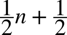
To understand the performance of Sequential Search, we must know how many elements it examines “on average.” Since v is known to be in the list and each element is equally likely to be v, the average number of examined elements, E(n), is the sum of the number of elements examined for each of the n values divided by n. Mathematically:
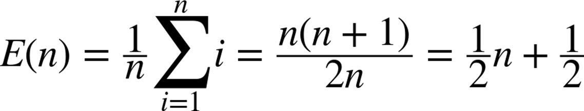
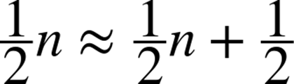
Thus, Sequential Search examines about half of the elements in a list of n distinct elements subject to these assumptions. If the number of elements in the list doubles, then Sequential Search should examine about twice as many elements; the expected number of probes is a linear function of n. That is, the expected number of probes is “about” c*n for some constant c; here, c = 0.5. A fundamental fact of performance analysis is that the constant c is unimportant in the long run, because the most important cost factor is the size of the problem instance, n. As n gets larger and larger, the error in claiming that:
becomes less significant. In fact, the ratio between the two sides of this approximation approaches 1. That is:
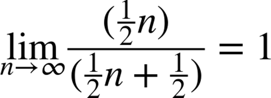
although the error in the estimation is significant for small values of n. In this context, we say the rate of growth of the expected number of elements that Sequential Search examines is linear. That is, we ignore the constant multiplier and are concerned only when the size of a problem instance is large.
When using the abstraction of the rate of growth to choose between algorithms, remember that:
Constants matter
That’s why we use supercomputers and upgrade our computers on a regular basis.
Size of n is not always large
We will see in Chapter 4 that the rate of growth of the execution time of Quicksort is less than the rate of growth of the execution time of Insertion Sort. Yet Insertion Sort outperforms Quicksort for small arrays on the same platform.
An algorithm’s rate of growth determines how it will perform on increasingly larger problem instances. Let’s apply this underlying principle to a more complex example.
Consider evaluating four sorting algorithms for a specific sorting task. The following performance data was generated by sorting a block of n random strings. For string blocks of size n = 1 – 512, 50 trials were run. The best and worst performances were discarded, and Figure 2-1 shows the average running time (in microseconds) of the remaining 48 results. The variance between the runs is surprising.
One way to interpret these results is to try to design a function that will predict the performance of each algorithm on a problem instance of size n. We are unlikely to guess such a function, so we use commercially available software to compute a trend line with a statistical process known as regression analysis. The “fitness” of a trend line to the actual data is based on a value between 0 and 1, known as the R2 value. R2 values near 1 indicate high fitness. For example, if R2 = 0.9948, there is only a 0.52% chance the fitness of the trend line is due to random variations in the data.
Sort-4 is clearly the worst performing of these sort algorithms. Given the 512 data points as plotted in a spreadsheet, the trend line to which its performance conforms is:
y = 0.0053*n2 – 0.3601*n + 39.212
R2 = 0.9948
Having an R2 confidence value so close to 1 declares this an accurate estimate. Sort-2 offers the fastest implementation over the given range of points. Its behavior is characterized by the following trend line equation:
y = 0.05765*n*log(n) + 7.9653
Sort-2 marginally outperforms Sort-3 initially, and its ultimate behavior is perhaps 10% faster than Sort-3. Sort-1 shows two distinct behavioral patterns. For blocks of 39 or fewer strings, the behavior is characterized by:
y = 0.0016*n2 + 0.2939*n + 3.1838
R2 = 0.9761
However, with 40 or more strings, the behavior is characterized by:
y = 0.0798*n*log(n) + 142.7818
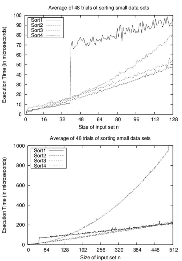
Figure 2-1. Comparing four sort algorithms on small data sets
The numeric coefficients in these equations are entirely dependent upon the platform on which these implementations execute. As described earlier, such incidental differences are not important. The long-term trend as n increases dominates the computation of these behaviors. Indeed,Figure 2-1 graphs the behavior using two different ranges to show that the real behavior for an algorithm may not be apparent until n is large enough.
Algorithm designers seek to understand the behavioral differences that exist between algorithms. Sort-1 reflects the performance of qsort on Linux 2.6.9. When reviewing the source code (which can be found through any of the available Linux code repositories), we discover the following comment: “Qsort routine from Bentley & McIlroy’s Engineering a Sort Function.” Bentley and McIlroy (1993) describe how to optimize Quicksort by varying the strategy for problem sizes less than 7, between 8 and 39, and for 40 and higher. It is satisfying to see that the empirical results presented here confirm the underlying implementation.
Analysis in the Best, Average, and Worst Cases
One question to ask is whether the results of the previous section will be true for all input problem instances. How will the behavior of Sort-2 change with different input problem instances of the same size?
§ The data could contain large runs of elements already in sorted order
§ The input could contain duplicate values
§ Regardless of the size n of the input set, the elements could be drawn from a much smaller set and contain a significant number of duplicate values
Although Sort-4 from Figure 2-1 was the slowest of the four algorithms for sorting n random strings, it turns out to be the fastest when the data is already sorted. This advantage rapidly fades away, however; with just 32 random items out of position, as shown in Figure 2-2, Sort-3 now has the best performance.
However, suppose an input array with n strings is “nearly sorted”—i.e., n/4 of the strings (25% of them) are swapped with another position just four locations away. It may come as a surprise to see in Figure 2-3 that Sort-4 outperforms the others.
The conclusion to draw is that for many problems, no single optimal algorithm exists. Choosing an algorithm depends on understanding the problem being solved and the underlying probability distribution of the instances likely to be treated, as well as the behavior of the algorithms being considered.
To provide some guidance, algorithms are typically presented with three common cases in mind:
Worst case
Defines a class of problem instances for which an algorithm exhibits its worst runtime behavior. Instead of trying to identify the specific input, algorithm designers typically describe properties of the input that prevent an algorithm from running efficiently.
Average case
Defines the expected behavior when executing the algorithm on random problem instances. While some instances will require greater time to complete because of some special cases, the vast majority will not. This measure describes the expectation an average user of the algorithm should have.
Best case
Defines a class of problem instances for which an algorithm exhibits its best runtime behavior. For these instances, the algorithm does the least work. In reality, the best case rarely occurs.
By knowing the performance of an algorithm under each of these cases, you can judge whether an algorithm is appropriate to use in your specific situation.
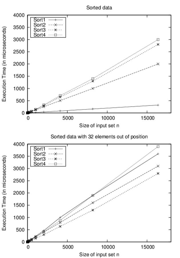
Figure 2-2. Comparing sort algorithms on sorted/nearly sorted data
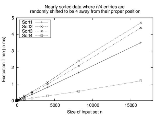
Figure 2-3. Sort-4 wins on nearly sorted data
Worst Case
For any particular value of n, the work done by an algorithm or program may vary dramatically over all the instances of size n. For a given program and a given value n, the worst-case execution time is the maximum execution time, where the maximum is taken over all instances of size n.
We are interested in the worst-case behavior of an algorithm because it often is the easiest case to analyze. It also explains how slow the program could be in any situation.
More formally, if Sn is the set of instances si of size n, and t() is a function that measures the work done by an algorithm on each instance, then work done by an algorithm on Sn in the worst case is the maximum of t(si) over all si ∈ Sn. Denoting this worst-case performance on Sn by Twc(n), the rate of growth of Twc(n) defines the worst-case complexity of the algorithm.
There are not enough resources to compute each individual instance si on which to run the algorithm to determine empirically the one that leads to worst-case performance. Instead, an adversary crafts a worst-case problem instance given the description of the algorithm.
Average Case
Consider a telephone system designed to support a large number n of telephones. In the worst case, it must be able to complete all calls where n/2 people pick up their phones and call the other n/2 people. Although this system will never crash because of overload, it would be prohibitively expensive to construct. In reality, the probability that each of n/2 people calls a unique member of the other n/2 people is exceedingly small. Instead, we could design a system that is cheaper to build and use mathematical tools to consider the probability of crash due to overload.
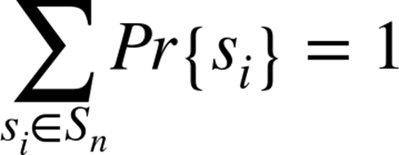
For the set of instances of size n, we associate a probability distribution Pr{si}, which assigns a probability between 0 and 1 to each instance si such that the sum of the probabilities over all instances of size n is 1. More formally, if Sn is the set of instances of size n, then:
If t() measures the work done by an algorithm on each instance, then the average-case work done by an algorithm on Sn is:
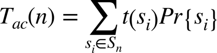
That is, the actual work done on instance si, t(si), is weighted with the probability that si will actually be presented as input. If Pr{si} = 0, then the actual value of t(si) does not impact the expected work done by the program. Denoting this average-case work on Sn by Tac(n), then the rate of growth of Tac(n) defines the average-case complexity of the algorithm.
Recall that when describing the rate of growth of work or time, we consistently ignore constants. So when we say that Sequential Search of n elements takes, on average:
probes (subject to our earlier assumptions), then by convention we simply say that subject to these assumptions, we expect Sequential Search will examine a linear number of elements, or order n.
Best Case
Knowing the best case for an algorithm is useful even though the situation rarely occurs in practice. In many cases, it provides insight into the optimal circumstance for an algorithm. For example, the best case for Sequential Search is when it searches for a desired value, v, which ends up being the first element in the list. Consider a slightly different approach, which we’ll call Counting Search, that counts the number of times that v appears in a list. If the computed count is zero, then the item was not found, so it returns false; otherwise, it returns true. Note that Counting Search always searches through the entire list; therefore, even though its worst-case behavior is O(n)—the same as Sequential Search—its best-case behavior remains O(n), so it is unable to take advantage of either the best-case or average-case situations in which it could have performed better.
Lower and Upper Bounds
We simplify the presentation of the “Big O” notation in this book. The goal is to classify the behavior of an algorithm as it solves problem instances of increasing size, n. The classification is stated as O(f(n)) where f(n) is most commonly a function such as n, n3, or 2n.
For example, assume there is an algorithm whose worst-case performance is never greater than directly proportional to the size of the input problem instance, once the size is “large enough.” More precisely, there exists some constant c > 0 such that t(n) ≤ c*n for all n > n0, where n0 is the point where each problem instance is “large enough.” In this case, the classification would be the function f(n) = n and we would use the notation O(n). For this same algorithm, assume that its best-case performance is never smaller than directly proportional to the size of the input problem instance. In this case, there exists a different constant c and a different threshold problem size, n0, and t(n) ≥ c*n for all n > n0. Here classification once again is f(n) = n and we would use the notation Ω(n).
To summarize, the actual formal notation is as follows:
§ The lower bound for the execution time of an algorithm is classified as Ω(f(n)) and corresponds to the best-case scenario
§ The upper bound for the execution time is classified as O(f(n)) and corresponds to the worst-case scenario
It is necessary to consider both scenarios. The careful reader will note that we could just as easily have used a function f(n) = c*2n to classify the algorithm discussed above as O(2n), though this describes much slower behavior. Indeed, doing so would provide little information—it would be like saying you need no more than 1 week to perform a 5-minute task. In this book, we always present an algorithm’s classification using its closest match.
In complexity theory, there is another notation, Θ(f(n)), which combines these concepts to identify an accurate tight bound—that is, when the lower bound is determined to be Ω(f(n)) and the upper bound is also O(f(n)) for the same classification f(n). We chose the widely accepted (and more informal use) of O(f(n)) to simplify the presentations and analyses. We ensure that when discussing algorithmic behavior, there is no more accurate f’(n) that can be used to classify the algorithms we identify as O(f(n)).
Performance Families
We compare algorithms by evaluating their performance on problem instances of size n. This methodology is the standard means developed over the past half-century for comparing algorithms. By doing so, we can determine which algorithms scale to solve problems of a nontrivial size by evaluating the running time needed by the algorithm in relation to the size of the provided input. A secondary performance evaluation is to consider how much memory or storage an algorithm needs; we address these concerns within the individual algorithm descriptions, as appropriate.
We use the following classifications, which are ordered by decreasing efficiency:
§ Constant: O(1)
§ Logarithmic: O(log n)
§ Sublinear: O(nd) for d < 1
§ Linear: O(n)
§ Linearithmic: O(n log n)
§ Quadratic: O(n2)
§ Exponential: O(2n)
When evaluating the performance of an algorithm, keep in mind that you must identify the most expensive computation within an algorithm to determine its classification. For example, consider an algorithm that is subdivided into two tasks, a task classified as linear followed by a task classified as quadratic. The overall performance of the algorithm must therefore be classified as quadratic.
We’ll now illustrate these performance classifications by example.
Constant Behavior
When analyzing the performance of the algorithms in this book, we frequently claim that some primitive operations provide constant performance. Clearly this claim is not an absolute determinant for the actual performance of the operation since we do not refer to specific hardware. For example, comparing whether two 32-bit numbers x and y are the same value should have the same performance regardless of the actual values of x and y. A constant operation is defined to have O(1) performance.
What about the performance of comparing two 256-bit numbers? Or two 1,024-bit numbers? It turns out that for a predetermined fixed size k, you can compare two k-bit numbers in constant time. The key is that the problem size (i.e., the values x and y being compared) cannot grow beyond the fixed size k. We abstract the extra effort, which is multiplicative in terms of k, using the notation O(1).
Log n Behavior
A bartender offers the following $10,000 bet to any patron: “I will choose a secret number from 1 to 1,000,000 and you will have 20 chances to guess my number. After each guess, I will either tell you Too Low, Too High, or You Win. If you guess my number in 20 or fewer questions, I give you $10,000. If none of your 20 guesses is my secret number you must give me $10,000.” Would you take this bet? You should, because you can always win. Table 2-1 shows a sample scenario for the range 1–8 that asks a series of questions, reducing the problem size by about half each time.
|
Number |
First round |
Second round |
Third round |
Fourth round |
|
1 |
Is it 4? Too High |
Is it 2? Too High |
Must be 1! You Win |
|
|
2 |
Is it 4? Too High |
Is it 2? You Win |
||
|
3 |
Is it 4? Too High |
Is it 2? Too Low |
Must be 3! You Win |
|
|
4 |
Is it 4? You Win |
|||
|
5 |
Is it 4? Too Low |
Is it 6? Too High |
Must be 5! You Win |
|
|
6 |
Is it 4? Too Low |
Is it 6? You Win |
||
|
7 |
Is it 4? Too Low |
Is it 6? Too Low |
Is it 7? You Win |
|
|
8 |
Is it 4? Too Low |
Is it 6? Too Low |
Is it 7? Too Low |
Must be 8! You Win |
|
Table 2-1. Sample behavior for guessing number from 1–8 |
||||
In each round, depending upon the specific answers from the bartender, the size of the potential range containing the secret number is cut in about half each time. Eventually, the range of the secret number will be limited to just one possible number; this happens after 1 + ⌊log2 (n)⌋ rounds, where log2(x) computes the logarithm of x in base 2. The floor function ⌊x⌋ rounds the number x down to the largest integer smaller than or equal to x. For example, if the bartender chooses a number between 1 and 10, you could guess it in 1 + ⌊log2 (10)⌋ = 1 + ⌊3.32⌋, or four guesses. As further evidence of this formula, if the bartender chooses one of two numbers, then you need two rounds to guarantee that you will guess the number, or 1 + ⌊log2 (2)⌋ = 1 + 1 = 2. Remember, according to the bartender’s rules, you must guess the number out loud.
This same approach works equally well for 1,000,000 numbers. In fact, the Guessing algorithm shown in Example 2-1 works for any range [low, high] and determines the value of the hidden number, n, in 1 + ⌊log2 (high-low + 1)⌋ rounds. If there are 1,000,000 numbers, this algorithm will locate the number in at most 1 + ⌊log2 (1,000,000)⌋ = 1 + ⌊19.93⌋, or 20 guesses (the worst case).
Example 2-1. Java code to guess number in range [low, high]
// Compute number of turns when n is guaranteed to be in range [low,high].
public static int turns (int n, int low, int high) {
int turns = 0;
// Continue while there is a potential number to guess
while (high >= low) {
turns++;
int mid = (low + high)/2;
if (mid == n) {
return turns;
} else if (mid < n) {
low = mid + 1;
} else {
high = mid - 1;
}
}
return turns;
}
Logarithmic algorithms are extremely efficient because they rapidly converge on a solution. These algorithms succeed because they reduce the size of the problem by about half each time. The Guessing algorithm reaches a solution after at most k = 1 + ⌊log2 (n)⌋ iterations, and at the ithiteration (0 < i ≤ k), the algorithm computes a guess that is known to be within ±ϵ = 2k–i – 1 from the actual hidden number. The quantity ϵ is considered the error, or uncertainty. After each iteration of the loop, ϵ is cut in half.
For the remainder of this book, whenever we refer to log (n) it is assumed to be computed in base 2, so we will drop the subscript log2 (n).
Another example showing efficient behavior is the Bisection algorithm, which computes a root of an equation in one variable; namely, for what values of x does a continuous function f(x) = 0? You start with two values, a and b, for which f(a) and f(b) are opposite signs—that is, one is positive and one is negative. At each step, the method bisects the range [a, b] by computing its midpoint, c, and determines in which half the root must lie. Thus, with each round, c approximates a root value and the method cuts the error in half.
To find a root of f(x) = x*sin(x) – 5*x – cos(x), start with a = –1 and b = 1. As shown in Table 2-2, the algorithm converges on the solution of f(x) = 0, where x = –0.189302759 is a root of the function.
|
n |
a |
b |
c |
f(c) |
|
1 |
–1 |
1 |
0 |
–1 |
|
2 |
–1 |
0 |
–0.5 |
1.8621302 |
|
3 |
–0.5 |
0 |
–0.25 |
0.3429386 |
|
4 |
–0.25 |
0 |
–0.125 |
–0.3516133 |
|
5 |
–0.25 |
–0.125 |
–0.1875 |
–0.0100227 |
|
6 |
–0.25 |
–0.1875 |
–0.21875 |
0.1650514 |
|
7 |
–0.21875 |
–0.1875 |
–0.203125 |
0.0771607 |
|
8 |
–0.203125 |
–0.1875 |
–0.1953125 |
0.0334803 |
|
9 |
–0.1953125 |
–0.1875 |
–0.1914062 |
0.0117066 |
|
10 |
–0.1914062 |
–0.1875 |
–0.1894531 |
0.0008364 |
|
11 |
–0.1894531 |
–0.1875 |
–0.1884766 |
–0.0045945 |
|
12 |
–0.1894531 |
–0.1884766 |
–0.1889648 |
–0.0018794 |
|
13 |
–0.1894531 |
–0.1889648 |
–0.189209 |
–0.0005216 |
|
14 |
–0.1894531 |
–0.189209 |
–0.1893311 |
0.0001574 |
|
15 |
–0.1893311 |
–0.189209 |
–0.18927 |
–0.0001821 |
|
16 |
–0.1893311 |
–0.18927 |
–0.1893005 |
–0.0000124 |
|
Table 2-2. Bisection method |
||||
Sublinear O(nd) Behavior for d < 1
In some cases, the behavior of an algorithm is better than linear, yet not as efficient as logarithmic. As discussed in Chapter 10, a k-d tree in multiple dimensions can partition a set of n d-dimensional points efficiently. If the tree is balanced, the search time for range queries that conform to the axes of the points is O(n1–1/d). For two-dimensional queries, the resulting performance is O(sqrt(n)).
Linear Performance
Some problems clearly seem to require more effort to solve than others. A child can evaluate 7 + 5 to get 12. How much harder is the problem 37 + 45?
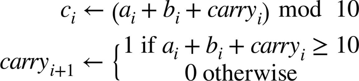
Specifically, how hard is it to add two n-digit numbers an–1…a0 + bn–1…b0 to result in an n + 1-digit number cn…c0 digit value? The primitive operations used in this Addition algorithm are as follows:
A sample Java implementation of Addition is shown in Example 2-2, where an n-digit number is represented as an array of int values whose most significant (i.e., leftmost) digit is in index position 0. For the examples in this section, it is assumed that each of these values is a decimal digitd such that 0 ≤ d ≤9.
Example 2-2. Java implementation of add
public static void add (int[] n1, int[] n2, int[] sum) {
int position = n1.length-1;
int carry = 0;
while (position >= 0) {
int total = n1[position] + n2[position] + carry;
sum[position+1] = total % 10;
if (total > 9) { carry = 1; } else { carry = 0; }
position--;
}
sum[0] = carry;
}
As long as the input problem can be stored in memory, add computes the addition of the two numbers as represented by the input integer arrays n1 and n2 and stores the result in the array sum. Would this implementation be as efficient as the following plus alternative, listed in Example 2-3, which computes the exact same answer using different computations?
Example 2-3. Java implementation of plus
public static void plus(int[] n1, int[] n2, int[] sum) {
int position = n1.length;
int carry = 0;
while (--position >= 0) {
int total = n1[position] + n2[position] + carry;
if (total > 9) {
sum[position+1] = total-10;
carry = 1;
} else {
sum[position+1] = total;
carry = 0;
}
}
sum[0] = carry;
}
Do these small implementation details affect the performance of an algorithm? Let’s consider two other potential factors that can impact the algorithm’s performance:
§ add and plus can trivially be converted into C programs. How does the choice of language affect the algorithm’s performance?
§ The programs can be executed on different computers. How does the choice of computer hardware affect the algorithm’s performance?
The implementations were executed 10,000 times on numbers ranging from 256 digits to 32,768 digits. For each digit size, a random number of that size was generated; thereafter, for each of the 10,000 trials, these two numbers were circular shifted (one left and one right) to create two different numbers to be added. Two different programming languages were used (C and Java). We start with the hypothesis that as the problem size doubles, the execution time for the algorithm doubles as well. We would like to know that this overall behavior occurs regardless of the machine, programming language, or implementation variation used. Each variation was executed on a set of configurations:
g
C version was compiled with debugging information included.
O1, O2, O3
C version was compiled under these different optimization levels. Increasing numbers imply better performance.
Java
Java implementation of algorithm.
Table 2-3 contains the results for both add and plus. The eighth and final column compares the ratio of the performance of plus on problems of size 2n versus problems of size n. Define t(n) to be the actual running time of the Addition algorithm on an input of size n. This growth pattern provides empirical evidence of the time to compute plus for two n-digit numbers.
|
n |
Add-g |
Add-java |
Add-O3 |
Plus-g |
Plus-java |
Plus-O3 |
Ratio |
|
256 |
33 |
19 |
10 |
31 |
20 |
11 |
|
|
512 |
67 |
22 |
20 |
58 |
32 |
23 |
2.09 |
|
1024 |
136 |
49 |
40 |
126 |
65 |
46 |
2.00 |
|
2048 |
271 |
98 |
80 |
241 |
131 |
95 |
2.07 |
|
4096 |
555 |
196 |
160 |
489 |
264 |
195 |
2.05 |
|
8192 |
1107 |
392 |
321 |
972 |
527 |
387 |
1.98 |
|
16384 |
2240 |
781 |
647 |
1972 |
1052 |
805 |
2.08 |
|
32768 |
4604 |
1554 |
1281 |
4102 |
2095 |
1721 |
2.14 |
|
65536 |
9447 |
3131 |
2572 |
8441 |
4200 |
3610 |
2.10 |
|
131072 |
19016 |
6277 |
5148 |
17059 |
8401 |
7322 |
2.03 |
|
262144 |
38269 |
12576 |
10336 |
34396 |
16811 |
14782 |
2.02 |
|
524288 |
77147 |
26632 |
21547 |
69699 |
35054 |
30367 |
2.05 |
|
1048576 |
156050 |
51077 |
53916 |
141524 |
61856 |
66006 |
2.17 |
|
Table 2-3. Time (in milliseconds) to execute 10,000 add/plus invocations on random digits of size n |
|||||||
We can classify the Addition algorithm as being linear with respect to its input size n. That is, there is some constant c > 0 such that t(n) ≤ c*n for “large enough” n, or more precisely, all n > n0. We don’t actually need to compute the actual value of c or n0; we just know they exist and they can be computed. An argument can be made to establish a linear-time lower bound on the complexity of Addition by showing that every digit must be examined (consider the consequences of not checking one of the digits).
For all plus executions (regardless of language or compilation configuration) of Addition, we can set c to 1/7 and choose n0 to be 256. Other implementations of Addition would have different constants, yet their overall behavior would still be linear. This result may seem surprising given that most programmers assume integer arithmetic is a constant time operation; however, constant time addition is achievable only when the integer representation (such as 16-bit or 64-bit) uses a fixed integer size n.
When considering differences in algorithms, the constant c is not as important as knowing the rate of growth of the algorithm. Seemingly inconsequential differences result in different performance. The plus implementation of Addition attempts to improve efficiency by eliminating the modulo operator (%). Still, when compiling both plus and add using -O3 optimization, add is nearly 30% faster. This is not to say that we ignore the value of c. Certainly if we execute Addition a large number of times, even small changes to the actual value of c can have a large impact on the performance of a program.
Linearithmic Performance
A common behavior in efficient algorithms is best described by this performance family. To explain how this behavior occurs in practice, let’s define t(n) to represent the time an algorithm takes to solve an input problem instance of size n. Divide and Conquer is an efficient way to solve a problem in which a problem of size n is divided into (roughly equal) subproblems of size n/2, which are solved recursively. The solutions of these subproblems are combined together in linear time to solve the original problem of size n. Mathematically, this can be stated as:
t(n) = 2*t(n/2) + c*n
That is, t(n) includes the cost of the two subproblems together with no more than a linear time cost (i.e., c*n) to merge the results. Now, on the right side of the equation, t(n/2) is the time to solve a problem of size n/2; using the same logic, this can be represented as:
t(n/2) = 2*t(n/4) + c*n/2
and so the original equation is now:
t(n) = 2*[2*t(n/4) + c*n/2] + c*n
If we expand this out once more, we see that:
t(n) = 2*[2*[2*t(n/8) + c*n/4] + c*n/2] + c*n
This last equation reduces to t(n) = 8*t(n/8) + 4*c*n/4 + 2*c*n/2 + c*n, which can be simplified as 8*t(n/8) + 3*c*n. We can then say that t(n) = (2k)*t(n/2k) + k*c*n. This expansion ends when 2k = n (i.e., when k = log(n)). In the final base case when the problem size is 1, the performancet(1) is a constant d. Thus, the closed-form formula for t(n) = n*d + c*n*log(n). Because c*n*log(n) is asymptotically greater than d*n for any fixed constants c and d, t(n) can be simply written as O(n log n).
Quadratic Performance
Now consider a similar problem where two integers of size n are multiplied together. Example 2-4 shows an implementation of Multiplication, an elementary school algorithm, using the same n-digit representation used earlier when adding numbers.
Example 2-4. mult implementation of Multiplication in Java
public static void mult (int[] n1, int[] n2, int[] result) {
int pos = result.length-1;
// clear all values
for (int i = 0; i < result.length; i++) { result[i] = 0; }
for (int m = n1.length-1; m>=0; m--) {
int off = n1.length-1 - m;
for (int n = n2.length-1; n>=0; n--,off++) {
int prod = n1[m]*n2[n];
// compute partial total by carrying previous digit's position
result[pos-off] += prod % 10;
result[pos-off-1] += result[pos-off]/10 + prod/10;
result[pos-off] %= 10;
}
}
}
Once again, an alternative program is written, times, which eliminates the need for the costly modulo operator, and skips the innermost computations when n1[m] is zero (note that times is not shown here, but can be found in the provided code repository). The times variation contains 203 lines of generated Java code to remove the two modulo operators. Does this variation show cost savings that validate the extra maintenance and development cost in managing this generated code?
Table 2-4 shows the behavior of these implementations of Multiplication using the same random input set used when demonstrating Addition. Figure 2-4 graphically depicts the performance, showing the parabolic growth curve that is the trademark of quadratic behavior.
|
n |
multn(ms) |
timesn(ms) |
mult2n/multn |
|
4 |
2 |
41 |
|
|
8 |
8 |
83 |
4 |
|
16 |
33 |
129 |
4.13 |
|
32 |
133 |
388 |
4.03 |
|
64 |
530 |
1276 |
3.98 |
|
128 |
2143 |
5009 |
4.04 |
|
256 |
8519 |
19014 |
3.98 |
|
512 |
34231 |
74723 |
4.02 |
|
Table 2-4. Time (in milliseconds) to execute 10,000 multiplications |
|||
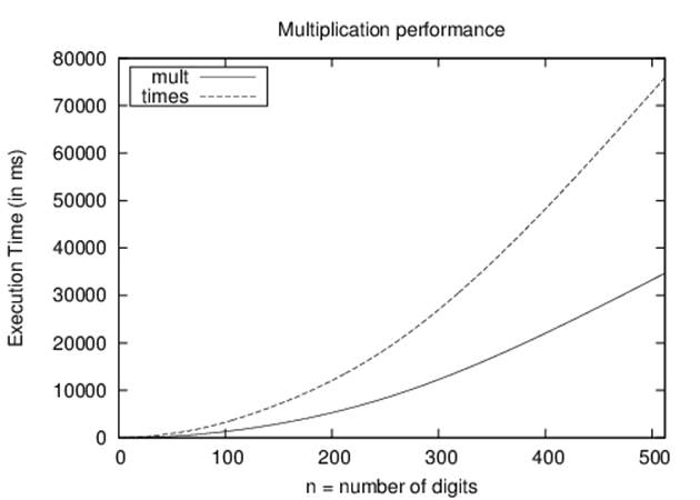
Figure 2-4. Comparison of mult versus times
Even though the times variation is twice as slow, both times and mult exhibit the same asymptotic performance. The ratio of mult2n/multn is roughly 4, which demonstrates that the performance of Multiplication is quadratic. Let’s define t(n) to be the actual running time of theMultiplication algorithm on an input of size n. By this definition, there must be some constant c > 0 such that t(n) ≤ c*n2 for all n > n0. We don’t actually need to know the full details of the c and n0 values, just that they exist. For the mult implementation of Multiplication on our platform, we can set c to 1/7 and choose n0 to be 16.
Once again, individual variations in implementation are unable to “break” the inherent quadratic performance behavior of an algorithm. However, other algorithms exist (Zuras, 1994) to multiply a pair of n-digit numbers that are significantly faster than quadratic. These algorithms are important for applications such as data encryption, in which one frequently multiplies large integers.
Less Obvious Performance Computations
In most cases, reading the description of an algorithm (as shown in Addition and Multiplication) is sufficient to classify an algorithm as being linear or quadratic. The primary indicator for quadratic, for example, is a nested loop structure. But some algorithms defy such straightforward analysis. Consider the GCD algorithm in Example 2-5, designed by Euclid to compute the greatest common divisor between two integers.
Example 2-5. Euclid’s GCD algorithm
public static void gcd (int a[], int b[], int gcd[]) {
if (isZero (a)) { assign (gcd, a); return; }
if (isZero (b)) { assign (gcd, b); return; }
a = copy (a); // Make copies to ensure
b = copy (b); // that a and b are not modified
while (!isZero (b)) {
// last argument to subtract represents sign of results which
// we can ignore since we only subtract smaller from larger.
// Note compareTo (a, b) is positive if a > b.
if (compareTo (a, b) > 0) {
subtract (a, b, gcd, new int[1]);
assign (a, gcd);
} else {
subtract (b, a, gcd, new int[1]);
assign (b, gcd);
}
}
// value held in a is the computed gcd of original (a,b)
assign (gcd, a);
}
This algorithm repeatedly compares two numbers (a and b) and subtracts the smaller number from the larger until zero is reached. The implementations of the helper methods (isZero, assign, compareTo, subtract) can be found in the accompanying code repository.
This algorithm produces the greatest common divisor of two numbers, but there is no clear answer as to how many iterations will be required based on the size of the input. During each pass through the loop, either a or b is reduced and never becomes negative, so we can guarantee that the algorithm will terminate, but some GCD requests take longer than others; for example, using this algorithm, gcd(1000,1) takes 999 steps! Clearly the performance of this algorithm is more sensitive to its inputs than Addition or Multiplication, in that there are different problem instances of the same size that require very different computation times. This GCD algorithm exhibits its worst-case performance when asked to compute the GCD of (10k–1, 1); it needs to process the while loop n = 10k–1 times! Since we have already shown that Addition is O(n) in terms of the input size n—and so is subtraction, by the way—GCD can be classified as O(n2).
The GCD implementation in Example 2-5 is outperformed handily by the ModGCD algorithm described in Example 2-6, which relies on the modulo operator to compute the integer remainder of a divided by b.
Example 2-6. ModGCD algorithm for GCD computation
public static void modgcd (int a[], int b[], int gcd[]) {
if (isZero(a)) { assign (gcd, a); return; }
if (isZero(b)) { assign (gcd, b); return; }
// align a and b to have same number of digits and work on copies
a = copy(normalize(a, b.length));
b = copy(normalize(b, a.length));
// ensure a is greater than b. Also return trivial gcd
int rc = compareTo(a,b);
if (rc == 0) { assign (gcd, a); return; }
if (rc < 0) {
int t[] = b;
b = a;
a = t;
}
int quot[] = new int[a.length];
int remainder[] = new int[a.length];
while (!isZero(b)) {
int t[] = copy (b);
divide (a, b, quot, remainder);
assign (b, remainder);
assign (a, t);
}
// value held in a is the computed gcd of (a,b).
assign (gcd, a);
}
ModGCD arrives at a solution more rapidly because it won’t waste time subtracting really small numbers from large numbers within the while loop. This difference is not simply an implementation detail; it reflects a fundamental shift in how the algorithm solves the problem.
The computations shown in Figure 2-5 (and enumerated in Table 2-5) show the result of generating 142 random n-digit numbers and computing the GCD of all 10,011 pairs of these numbers.
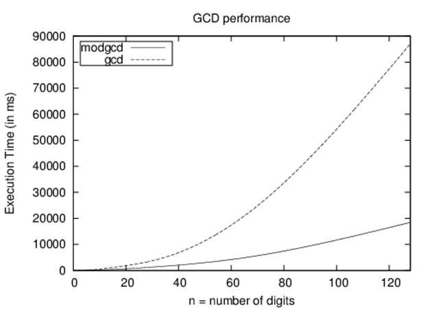
Figure 2-5. Comparison of gcd versus modgcd
|
n |
modgcd |
gcd |
modgcd2n/modgcdn |
|
4 |
68 |
45 |
0.23 |
|
8 |
226 |
408 |
3.32 |
|
16 |
603 |
1315 |
2.67 |
|
32 |
1836 |
4050 |
3.04 |
|
64 |
5330 |
18392 |
2.9 |
|
128 |
20485 |
76180 |
3.84 |
|
Table 2-5. Time (in milliseconds) to execute 10,011 gcd computations |
|||
Even though the ModGCD implementation is nearly three times faster than the corresponding GCD implementation on random computations, the performance of ModGCD is quadratic, or O(n2). The analysis is challenging and it turns out that the worst-case performance for ModGCD occurs for two successive Fibonacci numbers. Still, from Table 2-5 we can infer that the algorithm is quadratic because the performance appears to quadruple as the problem size doubles.
More sophisticated algorithms for computing GCD have been designed—though most are impractical except for extremely large integers—and analysis suggests that the problem allows for more efficient algorithms.
Exponential Performance
Consider a lock with three numeric dials in sequence, each of which contains the digits from 0 to 9. Each dial can be set independently to one of these 10 digits. Assume you have a found such a lock, but don’t have its combination; it is simply a matter of some manual labor to try each of the 1,000 possible combinations, from 000 to 999. To generalize this problem, assume the lock has n dials, then the total number of possibilities is 10n. Solving this problem using a brute-force approach would be considered exponential performance or O(10n), in this case in base 10. Often, the exponential base is 2, but this performance holds true for any base b > 1.
Exponential algorithms are practical only for very small values of n. Some algorithms might have a worst-case behavior that is exponential, yet still are heavily used in practice because of their average-case behavior. A good example is the Simplex algorithm for solving linear programming problems.
Summary of Asymptotic Growth
An algorithm with better asymptotic growth will eventually execute faster than one with worse asymptotic growth, regardless of the actual constants. The actual breakpoint will differ based on the actual constants, but it exists and can be empirically evaluated. In addition, during asymptotic analysis we only need to be concerned with the fastest-growing term of the t(n) function. For this reason, if the number of operations for an algorithm can be computed as c*n3 + d*n*log(n), we would classify this algorithm as O(n3) because that is the dominant term that grows far more rapidly than n*log(n).
Benchmark Operations
The Python operator ** rapidly performs exponentiation. The sample computation 2**851 is shown here.
150150336576094004599423153910185137226235191870990070733 557987815252631252384634158948203971606627616971080383694 109252383653813326044865235229218132798103200794538451818 051546732566997782908246399595358358052523086606780893692 34238529227774479195332149248
In Python, computations are relatively independent of the underlying platform (i.e., computing 2851 in Java or C on most platforms would cause numeric overflow). But a fast computation in Python yields the result shown in the preceding example. Is it an advantage or a disadvantage that Python abstracts away the underlying architecture? Consider the following two hypotheses:
Hypothesis H1
Computing 2n has consistent behavior, regardless of the value of n.
Hypothesis H2
Large numbers (such as shown previously in expanded form) can be treated in the same way as any other number, such as 123,827 or 997.
To refute hypothesis H1, we conduct 10,000 evaluations of 2n. The total execution time for each value of n is shown in Figure 2-6.
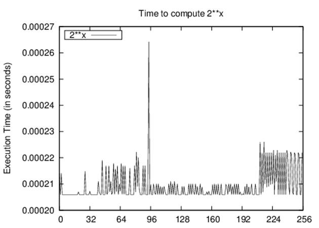
Figure 2-6. Execution times for computing 2x in Python
Oddly enough, the performance seems to have different behaviors, one for x smaller than 16, a second for x values around 145, and a third for x greater than 200. This behavior reveals that Python uses an Exponentiation By Squaring algorithm for computing powers using the ** operator. Manually computing 2x using a for loop would cause quadratic performance.
To refute hypothesis H2, we conduct an experiment that precomputes the value of 2n and then evaluates the time to compute π*2n. The total execution time of these 10,000 trials is shown in Figure 2-7.
Why do the points in Figure 2-7 not appear on a straight line? For what value of x does the line break? The multiplication operation (*) appears to be overloaded. It does different things depending on whether the numbers being multiplied are floating-point numbers, or integers that each fit into a single word of the machine, or integers that are so large they must each be stored in several words of the machine, or some combination of these.
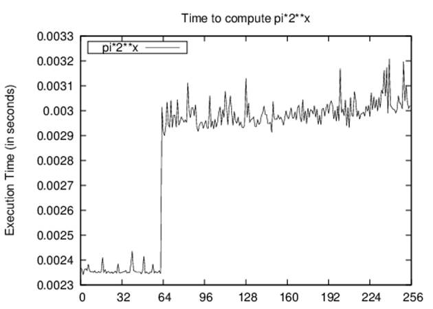
Figure 2-7. Execution times for computing large multiplication
The break in the plot occurs for x = {64,65} and appears to correspond to a shift in the storage of large floating-point numbers. Again, there may be unexpected slowdowns in computations that can only be uncovered by such benchmarking efforts.
References
Bentley, J., Programming Pearls. Second Edition. Addison-Wesley Professional, 1999.
Bentley, J. and M. McIlroy, “Engineering a sort function,” Software—Practice and Experience, 23(11): 1249–1265, 1993. http://dx.doi.org/10.1002/spe.4380231105
Zuras, D., “More on squaring and multiplying large integers,” IEEE Transactions on Computers, 43(8): 899–908, 1994, http://dx.doi.org/10.1109/12.295852.
All materials on the site are licensed Creative Commons Attribution-Sharealike 3.0 Unported CC BY-SA 3.0 & GNU Free Documentation License (GFDL)
If you are the copyright holder of any material contained on our site and intend to remove it, please contact our site administrator for approval.
© 2016-2026 All site design rights belong to S.Y.A.