Algorithms in a Nutshell: A Practical Guide (2016)

Chapter 7. Path Finding in AI

To solve a problem when there is no clear computation for a valid solution, we turn to path finding. This chapter covers two related path-finding approaches: one using game trees for two-player games and the other using search trees for single-player games. These approaches rely on a common structure, namely a state tree whose root node represents the initial state and edges represent potential moves that transform the state into a new state. The searches are challenging because the underlying structure is not computed in its entirety due to the explosion of the number of states. In a game of checkers, for example, there are roughly 5*10²⁰ different board configurations (Schaeffer, 2007). Thus, the trees over which the search proceeds are constructed on demand as needed. The two path-finding approaches are characterized as follows:

Game tree

Two players take turns alternating moves that modify the game state from its initial state. There are many states in which either player can win the game. There may also be some “draw” states in which no one wins. A path-finding algorithm maximizes the chance that a player will win or force a draw.

Search tree

A single player starts from an initial board state and makes valid moves until the desired goal state is reached. A path-finding algorithm identifies the exact sequence of moves that will transform the initial state into the goal state.

Game Trees

The game of tic-tac-toe is played on a 3×3 board where players take turns placing X and O marks on the board. The first player to place three of his marks in a row wins; the game is a draw if no spaces remain and no player has won. In tic-tac-toe there are only 765 unique positions (ignoring reflections and rotations of the board state) and a calculated 26,830 possible games that can be played (Schaeffer, 2002). To see some of the potential games, construct a game tree, as shown partially in Figure 7-1, and find a path from player O’s current game state (represented as the top node in this tree) to some future game state that ensures either a victory or a draw for player O.

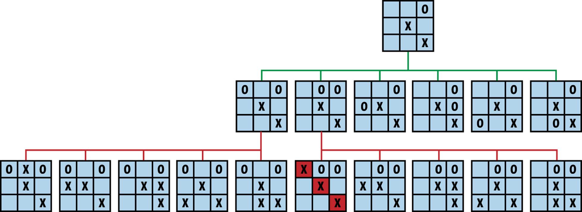
Figure 7-1. Partial game tree given an initial tic-tac-toe game state

A game tree is also known as an AND/OR tree since it is formed by two different types of nodes. The top node is an OR node, because the goal is for player O to select just one of the six available moves in the middle tier. The middle-tier nodes are AND nodes, because the goal (from O’s perspective) is to ensure all countermoves by X (shown as children nodes in the bottom tier) will still lead to either a victory or a draw for O. The game tree in Figure 7-1 is only partially expanded because there are actually 30 different game states in the bottom tier.

In a sophisticated game, the game tree may never be computed fully because of its size. The goal of a path-finding algorithm is to determine from a game state the player’s move that maximizes (or even guarantees) his chance of winning the game. We thus transform an intelligent set of player decisions into a path-finding problem over the game tree. This approach works for games with small game trees, but it can also scale to solve more complex problems.

The American game of checkers is played on an 8×8 board with an initial set of 24 pieces (12 red and 12 black). For decades, researchers attempted to determine whether the opening player could force a draw or a win. Although it is difficult to compute exactly, the size of the game tree must be incredibly large. After nearly 18 years of computations (sometimes on as many as 200 computers), researchers at the University of Alberta, Canada, demonstrated that perfect play by both players leads to a draw (Schaeffer, 2007).

Path finding in artificial intelligence (AI) provides specific algorithms to tackle incredibly complex problems if they can be translated into a combinatorial game of alternating players. Early researchers in AI (Shannon, 1950) considered the challenge of building a chess-playing machine and developed two types of approaches for search problems that continue to define the state of the practice today:

Type A

Consider the various allowed moves for both players a fixed set of turns into the future, and determine the most favorable position that results for the original player. Then, select the initial move that makes progress in that direction.

Type B

Add some adaptive decision based on knowledge of the game rather than static evaluation functions. More explicitly, (a) evaluate promising positions as far ahead as necessary to find a stable position where the board evaluation truly reflects the strength of the resulting position, and (b) select appropriate available moves. This approach tries to prevent pointless possibilities from consuming precious time.

In this chapter, we describe the family of Type A algorithms that provides a general-purpose approach for searching a game tree to find the best move for a player in a two-player game. These algorithms include Minimax, AlphaBeta, and NegMax.

The algorithms discussed in this chapter become unnecessarily complicated if the underlying information is poorly modeled. Many of the examples in textbooks or on the Internet naturally describe these algorithms in the context of a particular game. However, it may be difficult to separate the arbitrary way in which the game is represented from the essential elements of these algorithms. For this reason, we intentionally designed a set of object-oriented interfaces to maintain a clean separation between the algorithms and the games. We’ll now briefly summarize the core interfaces in our implementation of game trees, which are illustrated in Figure 7-2.

The IGameState interface abstracts the essential concepts needed to conduct searches over a game state. It defines how to:

Interpret the game state

isDraw() determines whether the game concludes with neither player winning; isWin() determines whether the game is won.

Manage the game state

copy() returns an identical copy of the game state so moves can be applied without updating the original game state; equivalent(IGameState) determines whether two game state positions are equal.

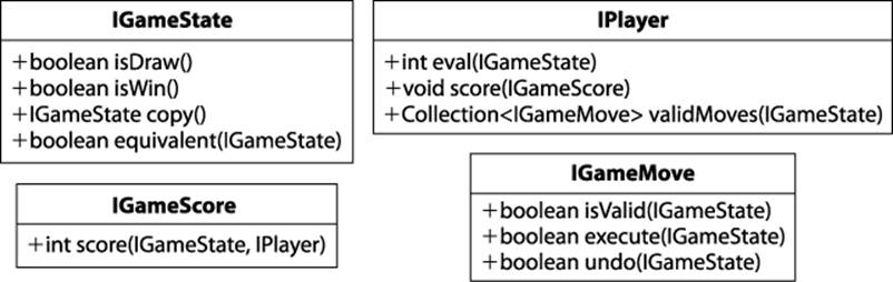
Figure 7-2. Core interfaces for game-tree algorithms

The IPlayer interface abstracts the abilities of a player to manipulate the game state. It defines how to:

Evaluate a board

eval(IGameState) returns an integer evaluating the game state from the player’s perspective; score(IGameScore) sets the scoring computation the player uses to evaluate a game state.

Generate valid moves

validMoves(IGameState) returns a collection of available moves given the game state.

The IGameMove interface defines how moves manipulate the game state. The move classes are problem-specific, and the search algorithm need not be aware of their specific implementation. IGameScore defines the interface for scoring states.

From a programming perspective, the heart of the path-finding algorithm for a game tree is an implementation of the IEvaluation interface shown in Example 7-1.

Example 7-1. Common interface for game-tree path finding

/**

* For game state, player and opponent, return the best move

* for player. If no move is even available, null is returned.

*/

public interface IEvaluation {

IGameMove bestMove(IGameState state, IPlayer player, IPlayer opponent);

}

Given a node representing the current game state, the algorithm computes the best move for a player assuming the opponent will play a perfect game in return.

Static Evaluation Functions

There are several ways to add intelligence to the search (Barr and Feigenbaum, 1981):

Select the order and number of allowed moves to be applied

When considering available moves at a game state, we should first evaluate the moves that are likely to lead to a successful outcome. In addition, we might discard specific moves that do not seem to lead to a successful outcome.

Select game states to “prune” from the search tree

As the search progresses, new knowledge may be discovered that can be used to eliminate game states that had (at one time) been selected to be part of the search.

The most common approach is to define static evaluation functions to evaluate the game state at intermediate points in the computation, and then order the set of available moves so that moves with a higher probability of leading to a solution are tried first. However, poor evaluation functions can prevent path-finding algorithms from selecting the best moves to make. As the saying goes, “garbage in, garbage out.”

A static evaluation function must take into account various features of the game-tree position to return an integer score that reflects the relative strength of the position from a player’s perspective. For example, the first successful program to play checkers, developed by Arthur Samuel (1959), evaluated board positions by considering two dozen features of a game, such as the “piece advantage feature” (comparing the number of pieces a player has versus her opponent) and a “winning trade feature” (trading pieces when winning but not when losing). Clearly, a more accurate evaluation function makes the game-solving engine a better player.

In this chapter, we use the BoardEvaluation scoring function for tic-tac-toe, which was defined by Nil Nilsson (1971). Let nc(gs, p) be the number of rows, columns, or diagonals on a tic-tac-toe game state, gs, in which player p may still get three in a row. We then define score(gs, p) to be:

§ +∞ if player p has won the game in game state gs

§ −∞ if the opponent of player p has won the game in game state gs

§ nc(gs, p) – nc(gs, opponent) if neither player has won the game in game state gs

Instead of restricting the evaluation to the current game state, an evaluation function could temporarily expand that state a fixed number of moves and select the move that may ultimately lead to a game state with maximum benefit to the player. This is frowned upon in practice because of (a) the cost in performing the operations, and (b) the sharing of code logic between the evaluation function and the search function, which breaks the clean separation between them.

Path-Finding Concepts

The following concepts apply to both two-player game trees and single-player search trees.

Representing State

Each node in a game or search tree contains all state information known at that position in the game. For example, in chess, the king can “castle” with the rook only if (a) neither piece has yet moved, (b) the intervening squares are empty and not currently attacked by an enemy piece, and (c) the king is not currently in check. Note that (b) and (c) can be computed directly from the board state and therefore do not need to be stored; however, the board state must separately store whether the king or rooks have moved.

For games with exponentially large trees, the state must be stored as compactly as possible. If symmetries exist in the state, such as with Connect Four, Othello, or the 15-puzzle, the tree can be greatly reduced by eliminating identical states that may simply be rotated or reflected. More complex representations called bitboards have been used for chess, checkers, or Othello to manage the incredibly large number of states with impressive efficiency gains (Pepicelli, 2005).

Calculating Available Moves

To find the best move, it must be possible at each state to compute the available moves allowed to the player making the move. The term branching factor refers to the total number of moves that are allowed at any individual state. The original 3×3 Rubik’s Cube has (on average) a branching factor of 13.5 (Korf, 1985). The popular children’s game Connect Four has a branching factor of 7 for most of the game. Checkers is more complicated because of the rule that a player must capture a piece if that move is available. Based on analyzing a large number of checkers databases, the branching factor for capture positions is 1.20, whereas for noncapture positions it is 7.94; Schaeffer (2008) computes the average branching factor in Checkers to be 6.14. The game of Go has an initial branching factor of 361 because it is played on a 19×19 board.

Algorithms are sensitive to the order by which the available moves are attempted. When the branching factor for a game is high but the moves are not properly ordered based on some evaluative measure of success, blindly searching a tree is inefficient.

Maximum Expansion Depth

Because of limited memory resources, some search algorithms limit the extent to which they expand the search and game trees. This approach has its weaknesses in games where a sequence of moves forms a calculated strategy. In chess, for example, a piece is often sacrificed for a potential advantage; if the sacrifice occurs at the edge of the maximum expansion, the advantageous game state would not be found. A fixed expansion depth leaves a “horizon” beyond which the search cannot see, often to the detriment of the success of the search. For single-player games, fixing the maximum depth means the algorithm will not find the solution that lies just beyond the horizon.

Minimax

Given a specific position in a game tree from the perspective of an initial player, a search program must find a move that leads to the greatest chance of victory (or at least a draw). Instead of considering only the current game state and the available moves at that state, the program must consider any countermoves that its opponent will make after it makes each move. The program assumes there is an evaluation function score(state, player) that returns an integer representing the score of the game state from player’s perspective; lower integer numbers (which may be negative) reflect weaker positions.

The game tree is expanded by considering future game states after a sequence of n moves have been made. Each level of the tree alternates between MAX levels (where the goal is to benefit the original player by maximizing the evaluated score of a game state) and MIN levels (where the goal is to benefit the opponent by minimizing the evaluated score of a game state). At alternating levels, then, the program selects a move that maximizes score(state, initial), but when the opponent is making its move, the program assumes the opponent will select a move that minimizesscore(state, initial).

Of course, the program can look ahead only a finite number of moves because the game tree is potentially infinite. The number of moves chosen to look ahead is called the ply. The trade-off is to select a suitable ply that leads to a search exploration that completes in reasonable time.

The following pseudocode illustrates the Minimax algorithm.

MINIMAX SUMMARY

Best, Average, Worst: O(b^ply)

bestmove (s, player, opponent)

original = player

[move, score] = minimax (s, ply, player, opponent)

return move

end

minimax (s, ply, player, opponent)

best = [null, null]

if ply is 0 orthere are no valid moves then

score = evaluate s for original player

return [null, score]

foreach valid move m for player in state s do

execute move m on s

[move, score] = minimax(s, ply-1, opponent, player)

undo move m on s

if player is original then

if score > best.score then best = [m, score]

else

if score < best.score then best = [m, score]

return best

end

Remember original player since evaluation is always from that player’s perspective.

If no more moves remain, player might have won (or lost), which is equivalent to reaching target ply depth.

With each recursive call, swap player and opponent to reflect alternating turns.

Successive levels alternate between MAX or MIN.

Figure 7-3 shows an evaluation of a move using Minimax with ply depth of 3. The bottom row of the game tree contains the five possible game states that result after the player makes a move, the opponent responds, and then the player makes a move. Each of these game states is evaluated from the point of view of the original player, and the integer rating is shown in each node. The MAX second row from the bottom contains internal nodes whose scores are the maximum of their respective children. From the point of view of the original player, these represent the best scores he can attain. However, the MIN third row from the bottom represents the worst positions the opponent can force on the player, thus its scores are the minimum of its children. As you can see, each level alternates between selecting the maximum and minimum of its children. The final score demonstrates that the original player can force the opponent into a game state that evaluates to 3.

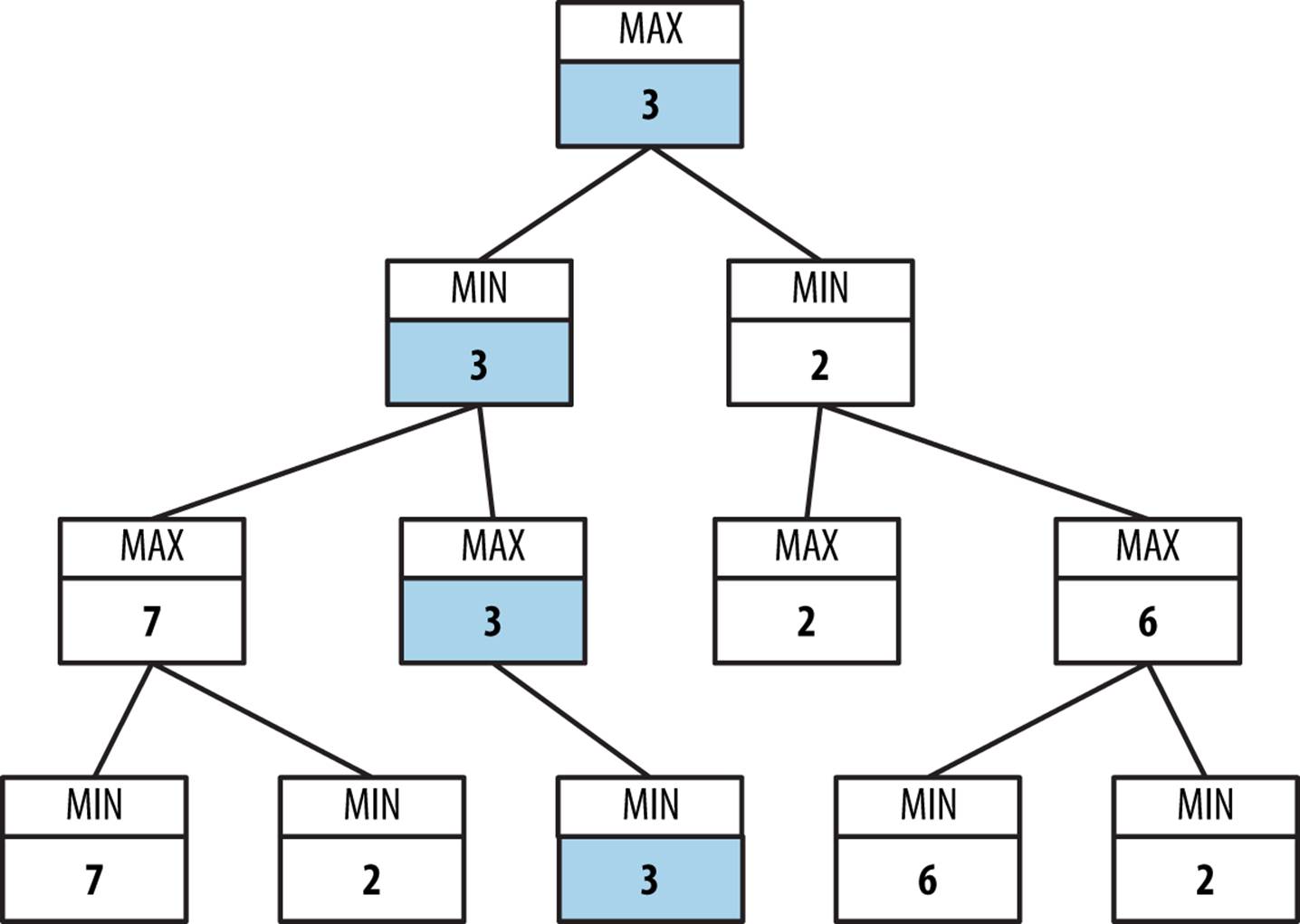
Figure 7-3. Minimax sample game tree

Input/Output

Minimax looks ahead a fixed number of moves, which is called the ply depth.

Minimax returns a move from among the valid moves that leads to the best future game state for a specific player, as determined by the evaluation function.

Context

Evaluating the game state is complex, and we must resort to heuristic evaluations to determine the better game state. Indeed, developing effective evaluation functions for games such as chess, checkers, or Othello is the greatest challenge in designing intelligent programs. We assume these evaluation functions are available.

The size of the game tree is determined by the number of available moves, b, at each game state. For most games, we can only estimate the value of b. For tic-tac-toe (and other games such as Nine Men’s Morris) there are b available moves in the initial empty game state, and each move takes away a potential move from the opponent. If the ply depth is d, the number of game states checked for tic-tac-toe is

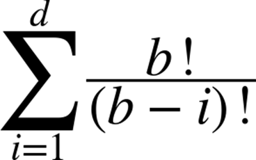
where b! is the factorial of b. To give an example of the scale involved, Minimax evaluates 187,300 states when b = 10 and d = 6.

During the recursive invocation within Minimax, the score(state, player) evaluation function must be consistently applied using the original player for whom a move is being calculated. This coordinates the minimum and maximum recursive evaluations.

Solution

The helper class MoveEvaluation pairs together an IMove and an int evaluation to be associated with that move. Minimax explores to a fixed ply depth, or when a game state has no valid moves for a player. The Java code in Example 7-2 returns the best move for a player in a given game state.

Example 7-2. Minimax implementation

public class MinimaxEvaluation implements IEvaluation {

IGameState state; /** State to be modified during search. */

int ply; /** Ply depth. How far to continue search. */

IPlayer original; /** Evaluate all states from this perspective. */

public MinimaxEvaluation (int ply) {

this.ply = ply;

}

public IGameMove bestMove (IGameState s,

IPlayer player, IPlayer opponent) {

this.original = player;

this.state = s.copy();

MoveEvaluation me = minimax(ply, IComparator.MAX,

player, opponent);

return me.move;

}

MoveEvaluation minimax (int ply, IComparator comp,

IPlayer player, IPlayer opponent) {

// If no allowed moves or a leaf node, return game state score.

Iterator<IGameMove> it = player.validMoves (state).iterator();

if (ply == 0 || !it.hasNext()) {

return new MoveEvaluation (original.eval (state));

}

// Try to improve on this lower bound (based on selector).

MoveEvaluation best = new MoveEvaluation (comp.initialValue());

// Generate game states resulting from valid moves for player

while (it.hasNext()) {

IGameMove move = it.next();

move.execute(state);

// Recursively evaluate position. Compute Minimax and swap

// player and opponent, synchronously with MIN and MAX.

MoveEvaluation me = minimax (ply-1, comp.opposite(),

opponent, player);

move.undo(state);

// Select maximum (minimum) of children if we are MAX (MIN)

if (comp.compare (best.score, me.score) < 0) {

best = new MoveEvaluation (move, me.score);

}

}

return best;

}

}

The MAX and MIN selectors evaluate scores to properly select the maximum or minimum score as desired. This implementation is simplified by defining an IComparator interface, shown in Figure 7-4, that defines MAX and MIN and consolidates how they select the best move from their perspective. Switching between the MAX and MIN selector is done using the opposite() method. The worst score for each of these comparators is returned by initialValue().

Minimax can rapidly become overwhelmed by the sheer number of game states generated during the recursive search. In chess, where the average number of moves on a board is 30 (Laramée, 2000), looking ahead just five moves (i.e., b = 30, d = 5) requires evaluating up to 25,137,931 board positions, as determined by the expression:

Minimax can take advantage of symmetries in the game state, such as rotations or reflections of the board, by caching past states viewed (and their respective scores), but the savings are game-specific.

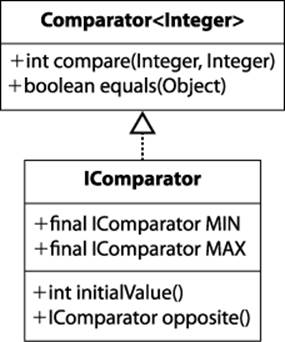
Figure 7-4. IComparator interface abstracts MAX and MIN operators

Figure 7-5 contains a two-ply exploration of an initial tic-tac-toe game state for player O using Minimax. The alternating levels of MAX and MIN show how the first move from the left—placing an O in the upper-left corner—is the only move that averts an immediate loss. Note that all possible game states are expanded, even when it becomes clear the opponent X can secure a win if O makes a poor move choice.

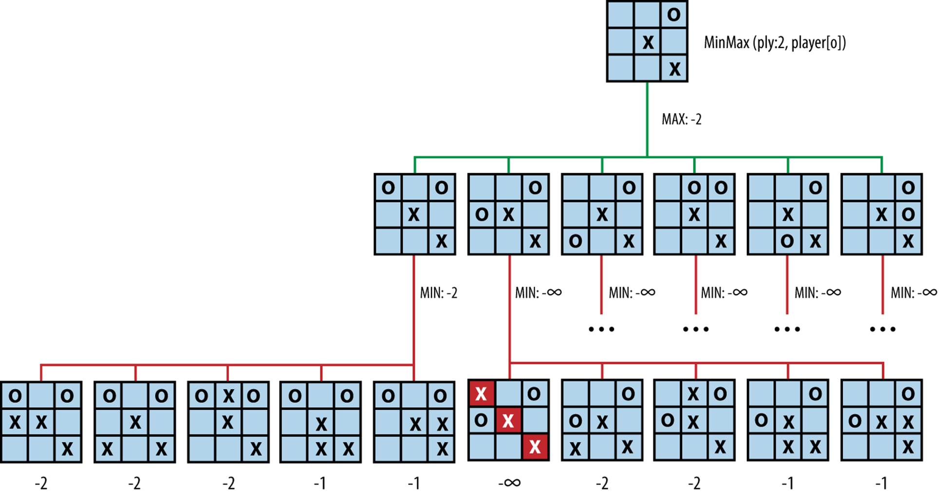
Figure 7-5. Sample Minimax exploration

Analysis

When there is a fixed number b of moves at each game state (or even when the number of available moves reduces by one with each level), the total number of game states searched in a d-ply Minimax is O(b^d), demonstrating exponential growth. The ply-depth restriction can be eliminated if the game tree is small enough to be completely evaluated in an acceptable amount of time.

Given the results of Figure 7-5, is there some way to eliminate exploring useless game states? Because we assume the player and opponent make no mistakes, we need to find a way to stop expanding the game tree once the algorithm determines that an entire subtree is worthless to explore further. AlphaBeta properly implements this capability; we first explain how to simplify the alternating MAX and MIN levels of the game tree with the NegMax algorithm.

NegMax

NegMax replaces the alternative MAX and MIN levels of Minimax with a single approach used at each level of the game tree. It also forms the basis of the AlphaBeta algorithm presented next.

In Minimax, the game state is always evaluated from the perspective of the player making the initial move (which requires the evaluation function to store this information). The game tree is thus composed of alternating levels that maximize the score of children nodes (when the original player) or minimize the score of children nodes (when the opponent). Instead, NegMax consistently seeks the move that produces the maximum of the negative values of a state’s children nodes.

NEGMAX SUMMARY

Best, Average, Worst: O(b^ply)

bestmove (s, player, opponent)

[move, score] = negmax (s, ply, player, opponent)

return move

end

negmax (s, ply, player, opponent)

best = [null, null]

if ply is 0 orthere are no valid moves then

score = evaluate s for player

return [null, score]

foreach valid move m for player in state s do

execute move m on s

[move, score] = negmax (s, ply-1, opponent, player)

undo move m on s

if -score > best.score then best = [m, -score]

return best

end

NegMax swaps players with each successive level.

Choose largest of the negative scores of its children.

Intuitively, after a player has made its move, the opponent will try to make its best move; thus, to find the best move for a player, select the one that restricts the opponent from scoring too highly. If you compare the pseudocode examples, you will see that Minimax and NegMax produce two game trees with identical structure; the only difference is how the game states are scored.

The structure of the NegMax game tree is identical to the Minimax game tree because it finds the exact same move; the only difference is that the values in levels previously labeled as MIN are negated in NegMax. If you compare the tree in Figure 7-6 with Figure 7-3, you see this behavior.

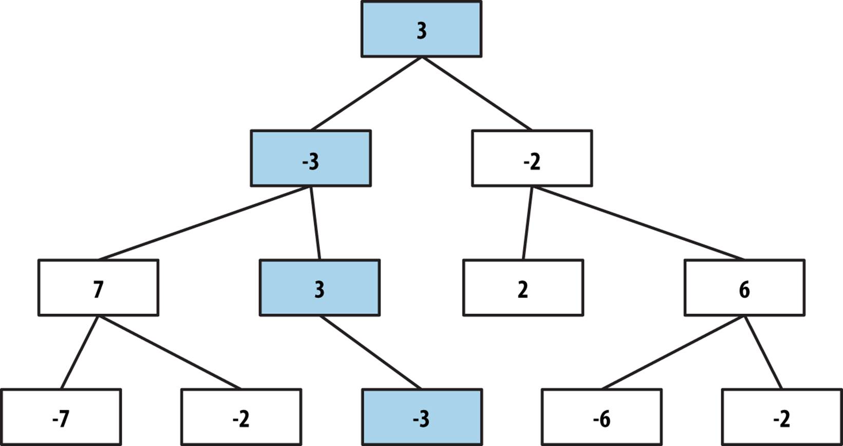
Figure 7-6. NegMax sample game tree

Solution

In Example 7-3, note that the score for each MoveEvaluation is simply the evaluation of the game state from the perspective of the player making that move. Reorienting each evaluation toward the player making the move simplifies the algorithm implementation.

Example 7-3. NegMax implementation

public class NegMaxEvaluation implements IEvaluation {

IGameState state; /** State to be modified during search. */

int ply; /** Ply depth. How far to continue search. */

public NegMaxEvaluation (int ply) {

this.ply = ply;

}

public IGameMove bestMove (IGameState s, IPlayer player, IPlayer opponent)

{

state = s.copy();

MoveEvaluation me = negmax (ply, player, opponent);

return me.move;

}

public MoveEvaluation negmax (int ply, IPlayer player, IPlayer opponent)

{

// If no allowed moves or a leaf node, return board state score.

Iterator<IGameMove> it = player.validMoves (state).iterator();

if (ply == 0 || !it.hasNext()) {

return new MoveEvaluation (player.eval (state));

}

// Try to improve on this lower-bound move.

MoveEvaluation best = new MoveEvaluation (MoveEvaluation.minimum());

// get moves for this player and generate the boards that result from

// these moves. Select maximum of the negative scores of children.

while (it.hasNext()) {

IGameMove move = it.next();

move.execute (state);

// Recursively evaluate position using consistent negmax.

MoveEvaluation me = negmax (ply-1, opponent, player);

move.undo (state);

if (-me.score > best.score) {

best = new MoveEvaluation (move, -me.score);

}

}

return best;

}

}

NegMax is useful because it prepares a simple foundation on which to extend to AlphaBeta. Because board scores are routinely negated in this algorithm, we must carefully choose values that represent winning and losing states. Specifically, the minimum value must be the negated value of the maximum value. Note that Integer.MIN_VALUE (defined in Java as 0x80000000 or −2,147,483,648) is not the negated value of Integer.MAX_VALUE (in Java, defined as 0x7fffffff or 2,147,483,647). For this reason, we use Integer.MIN_VALUE+1 as the minimum value, which is retrieved by the static function MoveEvaluation.minimum(). For completeness, we provide MoveEvaluation.maximum() as well.

Figure 7-7 contains a two-ply exploration of an initial tic-tac-toe game state for player O using NegMax. NegMax expands all possible game states, even when it becomes clear the opponent X can secure a win if O makes a poor move. The scores associated with each of the leaf game states are evaluated from that player’s perspective (in this case, the original player O). The score for the initial game state is −2, because that is the “maximum of the negative scores of its children.”

Analysis

The number of states explored by NegMax is the same as Minimax, on the order of b^d for a d-ply search with fixed number b of moves at each game state. In all other respects, it performs identically to Minimax.

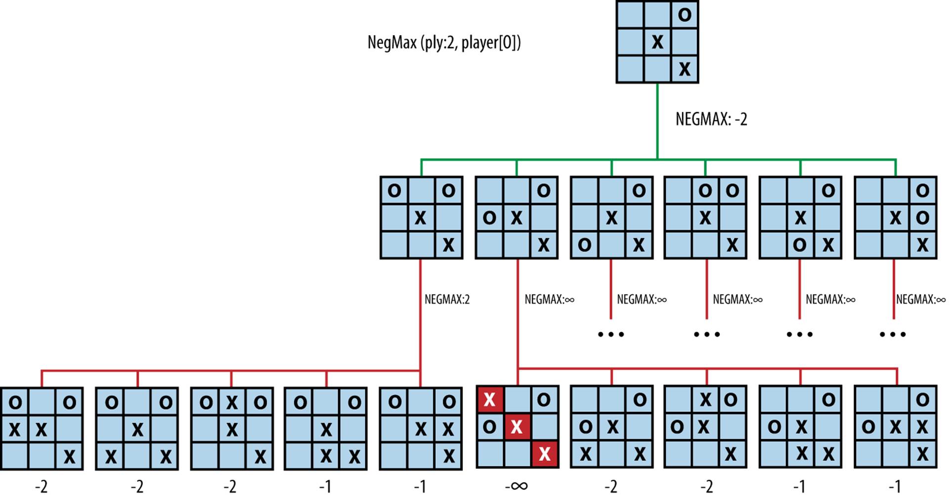
Figure 7-7. Sample NegMax exploration

AlphaBeta

Minimax evaluates a player’s best move when considering the opponent’s countermoves, but this information is not used while the game tree is generated! Consider the BoardEvaluation scoring function introduced earlier. Recall Figure 7-5, which shows the partial expansion of the game tree from an initial game state after X has made two moves and O has made just one move.

Note how Minimax plods along even though each subsequent search reveals a losing board if X is able to complete the diagonal. A total of 36 nodes are evaluated. Minimax takes no advantage of the fact that the original decision for O to play in the upper-left corner prevented X from scoring an immediate victory. AlphaBeta defines a consistent strategy to prune unproductive searches from the search tree.

After evaluating the sub game tree rooted at (1) in Figure 7-8, AlphaBeta knows that if this move is made the opponent cannot force a worse position than -3, which means the best the player can do is score a 3. When AlphaBeta gets to the game state (2), the first child game state (3) evaluates to 2. This means that if the move for (2) is selected, the opponent can force the player into a game state that is less than the best move found so far (i.e., 3). There is no need to check the sibling subtree rooted at (4), so it is pruned away.

Using AlphaBeta, the equivalent expansion of the game tree is shown in Figure 7-9.

As AlphaBeta searches for the best move in Figure 7-9, it remembers that X can score no higher than 2 if O plays in the upper-left corner. For each subsequent other move for O, AlphaBeta determines that X has at least one countermove that outperforms the first move for O (indeed, in all cases X can win). Thus, the game tree expands only 16 nodes, a savings of more than 50% from Minimax. AlphaBeta selects the same move that Minimax would have selected, with potentially significant performance savings.

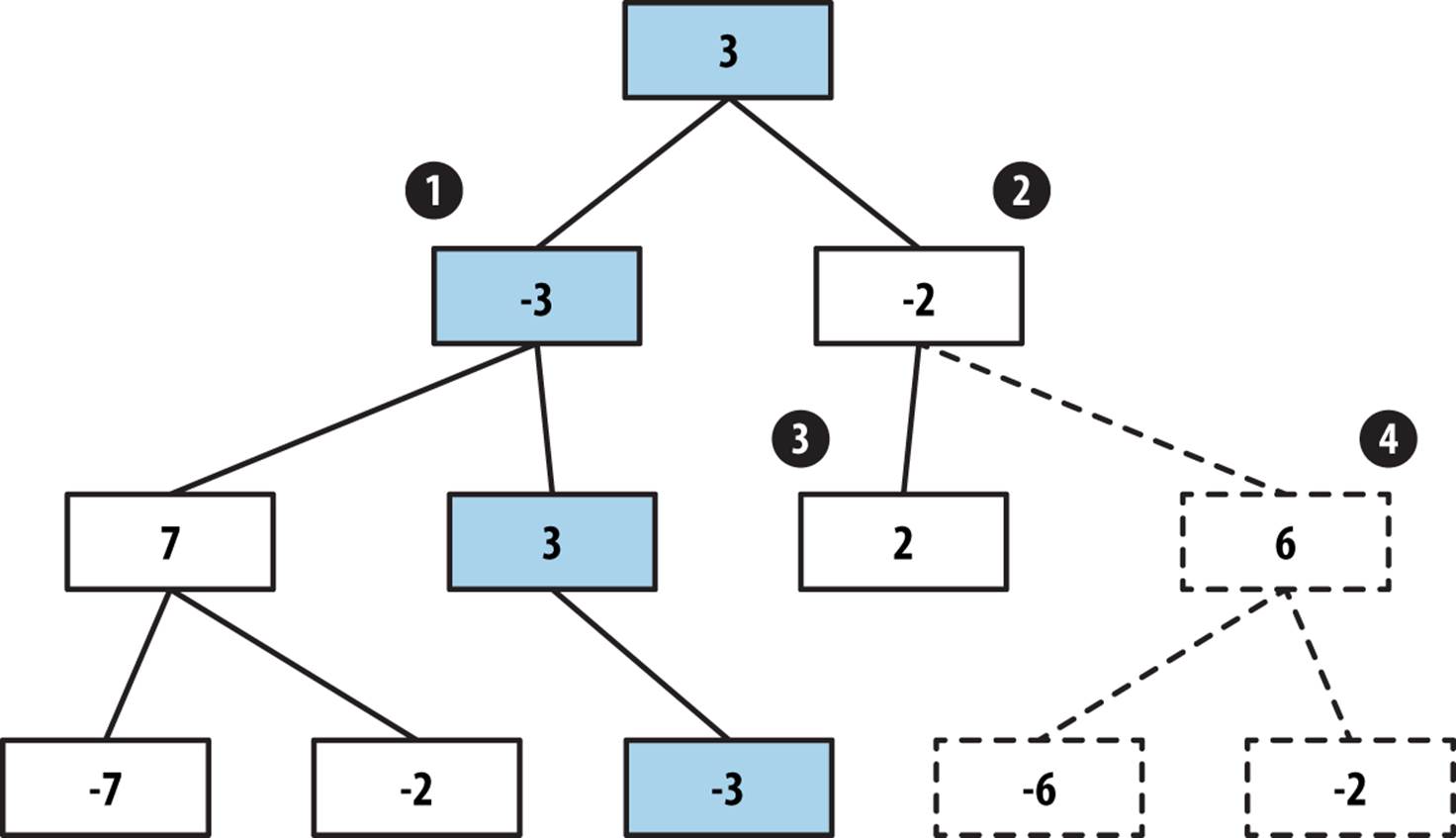
Figure 7-8. AlphaBeta sample game tree

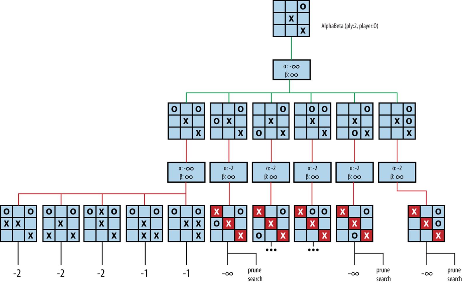
Figure 7-9. AlphaBeta two-ply search

AlphaBeta recursively searches through the game tree and maintains two values, α and β, which define a “window of opportunity” for a player as long as α < β. The value α represents the lower bound of the game states found for the player so far (or −∞ if none have been found) and declares that the player has found a move to ensure it can score at least that value. Higher values of α mean the player is doing well; when α = +∞, the player has won and the search can terminate.

The value β represents the upper bound of game states so far (or +∞ if none have been found) and declares the maximum value the player can achieve. When β drops lower and lower, the opponent is doing better at restricting the player’s options. Since AlphaBeta has a maximum ply depth beyond which it will not search, any decisions it makes are limited to this scope.

ALPHABETA SUMMARY

Best, Average: O(b^ply/2) Worst: O(b^ply)

bestmove (s, player, opponent)

[move, score] = alphaBeta (s, ply, player, opponent, -∞, ∞)

return move

end

alphaBeta (s, ply, player, opponent, low, high)

best = [null, null]

if ply is 0 orthere are no valid moves then

score = evaluate s for player

return [null, score]

foreach valid move m for player in state s do

execute move m on s

[move, score] = alphaBeta (s, ply-1, opponent, player, -high, -low)

undo move m on s

if -score > best.score then

low = -score

best = [m, -low]

if low ≥ high then return best

return best

end

At start, worst player can do is lose (low = –∞). Best player can do is win (high = +∞).

AlphaBeta evaluates leaf nodes as in NegMax.

Stop exploring sibling nodes when worst score possible by opponent equals or exceeds our maximum threshold.

The game tree in Figure 7-9 shows the [α, β] values as AlphaBeta executes; initially they are [–∞, ∞]. With a two-ply search, AlphaBeta is trying to find the best move for O when considering just the immediate countermove for X.

Because AlphaBeta is recursive, we can retrace its progress by considering a traversal of the game tree. The first move AlphaBeta considers is for O to play in the upper-left corner. After all five of X’s countermoves are evaluated, it is evident that X can ensure only a score of –2 for itself (using the static evaluation BoardEvaluation for tic-tac-toe). When AlphaBeta considers the second move for O (playing in the middle of the left column), its [α, β] values are now [–2, ∞], which means “the worst that O can end up with so far is a state whose score is –2, and the best that O can do is still win the game.” When the first countermove for X is evaluated, AlphaBeta detects that X has won, which falls outside of this “window of opportunity,” so further countermoves by X no longer need to be considered.

To explain how AlphaBeta prunes the game tree to eliminate nonproductive nodes, Figure 7-10 presents a three-ply search of Figure 7-5 that expands 66 nodes (whereas the corresponding Minimax game tree would require 156 nodes).

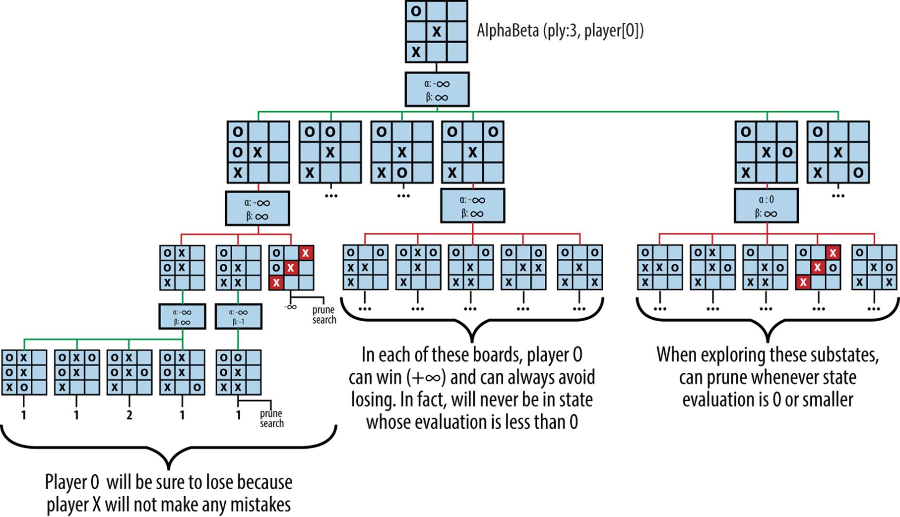
Figure 7-10. AlphaBeta three-ply search

At the initial node n in the game tree, player O must consider one of six potential moves. Pruning can occur on either the player’s turn or the opponent’s turn. In the search shown in Figure 7-10, there are two such examples:

Player’s turn

Assume O plays in the middle of the left column and X responds by playing in the middle of the top row (this is the leftmost grandchild of the root node in the search tree). From O’s perspective, the best score that O can force is –1 (note that in the diagram the scores are shown as 1 because AlphaBeta uses the same scoring mechanism used by NegMax). This value is remembered when it tries to determine what O can achieve if X had instead countered by playing in the middle of the bottom row. Note that [α, β] is now [–∞, –1]. AlphaBeta evaluates the result when O plays in the middle of the top row and computes the score 1. Because this value is greater than or equal to the –1 value, the remaining three potential moves for O in this level are ignored.

Opponent’s turn

Assume O plays in the middle of the left column and X responds by playing in the upper-right corner, immediately winning the game. AlphaBeta can ignore X’s two other potential moves, because O will prune the remaining nodes in the search subtree “rooted” in the decision to play in the middle of the left column.

The pruning of the search occurs when α ≥ β, or in other words, when the “window of opportunity” closes. When AlphaBeta is based on Minimax, there are two ways to prune the search, known as α-prune and β-prune; in the simpler AlphaBeta based on NegMax, these two cases are combined into the one discussed here. Because AlphaBeta is recursive, the range [α, β] represents the window of opportunity for the player, and the window of opportunity for the opponent is [–β, –α]. Within the recursive invocation of AlphaBeta the player and opponent are swapped, and the window is similarly swapped.

Solution

The AlphaBeta implementation in Example 7-4 augments NegMax by terminating early the evaluation of game states once it becomes clear that either the player can’t guarantee a better position (an α-prune) or the opponent can’t force a worse position (a β-prune).

Example 7-4. AlphaBeta implementation

public class AlphaBetaEvaluation implements IEvaluation {

IGameState state; /** State to be modified during search. */

int ply; /** Ply depth. How far to continue search. */

public AlphaBetaEvaluation (int ply) { this.ply = ply; }

public IGameMove bestMove (IGameState s,

IPlayer player, IPlayer opponent) {

state = s.copy();

MoveEvaluation me = alphabeta (ply, player, opponent,

MoveEvaluation.minimum(),

MoveEvaluation.maximum());

return me.move;

}

MoveEvaluation alphabeta (int ply, IPlayer player, IPlayer opponent,

int alpha, int beta) {

// If no moves, return board evaluation from player's perspective.

Iterator<IGameMove> it = player.validMoves (state).iterator();

if (ply == 0 || !it.hasNext()) {

return new MoveEvaluation (player.eval (state));

}

// Select "maximum of negative value of children" that improves alpha

MoveEvaluation best = new MoveEvaluation (alpha);

while (it.hasNext()) {

IGameMove move = it.next();

move.execute (state);

MoveEvaluation me = alphabeta (ply-1,opponent,player,-beta,-alpha);

move.undo (state);

// If improved upon alpha, keep track of this move.

if (-me.score > alpha) {

alpha = -me.score;

best = new MoveEvaluation (move, alpha);

}

if (alpha >= beta) { return best; } // search no longer productive.

}

return best;

}

}

The moves found will be exactly the same as those found by Minimax. But because many states are removed from the game tree as it is expanded, execution time is noticeably less for AlphaBeta.

Analysis

To measure the benefit of AlphaBeta over NegMax, we compare the size of their respective game trees. This task is complicated because AlphaBeta will show its most impressive savings if the opponent’s best move is evaluated first whenever AlphaBeta executes. When there is a fixed number b of moves at each game state, the total number of potential game states to search in a d-ply AlphaBeta is on the order of b^d. If the moves are ordered by decreasing favorability (i.e., the best move first), we still have to evaluate all b children for the initiating player (because we are to choose his best move); however, in the best case we need to evaluate only the first move by the opponent. Note in Figure 7-9 that, because of move ordering, the prune occurs after several moves have been evaluated, so the move ordering for that game tree is not optimal.

In the best case, therefore, AlphaBeta evaluates b game states for the initial player on each level, but only one game state for the opponent. So, instead of expanding b*b*b* … *b*b (a total of d times) game states on the d^th level of the game tree, AlphaBeta may require only b*1*b*…*b*1(a total of d times). The resulting number of game states is b^d/2, an impressive savings.

Instead of simply trying to minimize the number of game states, AlphaBeta could explore the same total number of game states as Minimax. This would extend the depth of the game tree to 2*d, thus doubling how far ahead the algorithm can look.

To empirically evaluate Minimax and AlphaBeta, we construct a set of initial tic-tac-toe board states that are possible after k moves have been made. We then compute Minimax and AlphaBeta with a ply of 9 – k, which ensures all possible moves are explored. The results are shown inTable 7-1. Observe the significant reduction of explored states using AlphaBeta.

Individual comparisons show the dramatic improvement of AlphaBeta; some of these cases explain why AlphaBeta is so powerful. For the game state shown in Figure 7-11, AlphaBeta explores only 450 game states (instead of 8,232 for Minimax, a 94.5% reduction) to determine that player X should select the center square, after which a win is assured.

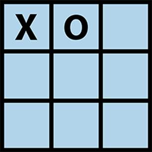
Figure 7-11. Sample tic-tac-toe board after two plays

However, the only way to achieve such deep reductions is if the available moves are ordered such that the best move appears first. Because our tic-tac-toe solution does not order moves in this fashion, some anomalies will result. For example, given the same board state rotated 180 degrees (Figure 7-12), AlphaBeta will explore 960 game states (an 88.3% reduction) because it expands the game tree using a different ordering of valid moves. For this reason, search algorithms often reorder moves using a static evaluation function to reduce the size of the game tree.

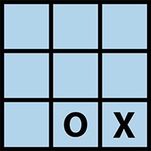
Figure 7-12. Sample tic-tac-toe board after two plays, rotated

Search Trees

Games that have just one player are similar to game trees, featuring an initial state (the top node in the search tree) and a sequence of moves that transforms the board state until a goal state is reached. A search tree represents the set of intermediate board states as a path-finding algorithm progresses. The computed structure is a tree because the algorithm ensures it does not visit a board state twice. The algorithm decides the order of board states to visit as it attempts to reach the goal.

We’ll explore search trees using an 8-puzzle, which is played on a 3×3 grid containing eight square tiles numbered 1 to 8 and an empty space that contains no tile. A tile adjacent (either horizontally or vertically) to the empty space can be moved by sliding it into the empty space. The aim is to start from a shuffled initial state and move tiles to achieve the goal state. The eight-move solution in Figure 7-13 is recorded as the bold path from the initial node to the goal node.

Figure 7-13. Sample 8-puzzle search

Search trees can rapidly explode to contain (potentially) billions or trillions of states. The algorithms in this chapter describe how to efficiently search through these trees more rapidly than using a blind search. To describe the inherent complexity of the problem, we introduce Depth-First Search and Breadth-First Search as two potential approaches to path-finding algorithms. We then present the powerful A*Search algorithm for finding a minimal-cost solution (under certain conditions). We’ll now briefly summarize the core classes, illustrated in Figure 7-14, that will be used when discussing search tree algorithms.

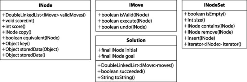
Figure 7-14. Core interfaces and classes for search-tree algorithms

The INode interface abstracts the essential concepts needed to conduct searches over a board state:

Generate valid moves

validMoves() returns a list of available moves for a board state.

Evaluate the board state

score(int) associates an integer score with the board state, representing the result of an evaluation function; score() returns the evaluation result previously associated with the board state.

Manage the board state

copy() returns an identical copy of the board state (except for the optional stored data); equivalent(INode) determines whether two board states are equal (sophisticated implementations may detect rotational symmetries in the board state or other means for equivalence). key()returns an object to support an equivalence check: if two board states have the same key() result, the board states are equivalent.

Managing optional board state data

storedData(Object o) associates the given object with the board state to be used by search algorithms; storedData() returns the optionally stored data that may be associated with the board state.

The INodeSet interface abstracts the underlying implementation of a set of INodes. Some algorithms require a queue of INode objects, some a stack, and others a balanced binary tree. Once properly constructed (using the StateStorageFactory class), the provided operations enable algorithms to manipulate the state of the INode set no matter the underlying data structure used. The IMove interface defines how moves can manipulate the board state; the specific move classes are problem-specific, and the search algorithm need not be aware of their specific implementation.

From a programming perspective, the heart of the path-finding algorithm for a search tree is the implementation of the ISearch interface shown in Example 7-5. Given such a solution, the moves that produced the solution can be extracted.

Example 7-5. Common interface for search-tree path finding

/**

* Given an initial state, return a Solution to the final

* state, or null if no such path can be found.

*/

public interface ISearch {

Solution search (INode initial, INode goal);

}

Given a node representing the initial board state and a desired goal node, an ISearch implementation computes a path representing a solution, or returns null if no solution was found. To differentiate from game trees, we use the term board state when discussing search tree nodes.

Path-Length Heuristic Functions

A blind-search algorithm uses a fixed strategy rather than evaluating the board state. A depth-first blind search simply plays the game forward by arbitrarily choosing the next move from available choices in that board state, backtracking when it hits its maximum expansion depth. A breadth-first blind search methodically explores all possible solutions with k moves before first attempting any solution with k + 1 moves. Surely there must be a way to guide the search based on the characteristics of the board states being investigated, right?

The discussion of A*Search will show searches over the 8-puzzle using different heuristic functions. These heuristic functions do not play the game, rather they estimate the number of remaining moves to a goal state from a given board state and can be used to direct the path-finding search. For example, in the 8-puzzle, such a function would evaluate for each tile in the board state the number of moves to position it in its proper location in the goal state. Most of the difficulty in path finding is crafting effective heuristic functions.

Depth-First Search

Depth-First Search attempts to locate a path to the goal state by making as much forward progress as possible. Because some search trees explore a high number of board states, Depth-First Search is practical only if a maximum search depth is fixed in advance. Furthermore, loops must be avoided by remembering each state and ensuring it is visited only once.

DEPTH-FIRST SEARCH SUMMARY

Best: O(b*d) Average, Worst: O(b^d)

search (initial, goal, maxDepth)

if initial = goal then return "Solution"

initial.depth = 0

open = new Stack

closed = new Set

insert (open, copy(initial))

while open is notempty do

n = pop (open)

insert (closed, n)

foreach valid move m at n do

nextState = state when playing m at n

if closed doesn't contain nextState then

nextState.depth = n.depth + 1

if nextState = goal then return "Solution"

if nextState.depth < maxDepth then

insert (open, nextState)

return "No Solution"

end

Depth-First Search uses a Stack to store open states to be visited.

Pop the most recent state from the stack.

Depth-First Search computes the depth to avoid exceeding maxDepth.

Inserting the next state will be a push operation since open is a stack.

Depth-First Search maintains a stack of open board states that have yet to be visited and a set of closed board states that have been visited. At each iteration, Depth-First Search pops from the stack an unvisited board state and expands it to compute the set of successor board states given the available valid moves. The search terminates if the goal state is reached. Any successor board states that already exist within the closed set are discarded. The remaining unvisited board states are pushed onto the stack of open board states and the search continues.

Figure 7-15 shows the computed search tree for an initial 8-puzzle board state using a depth limit of 9. Note how a path of 8 moves is found to the solution (marked as GOAL) after some exploration to depth 9 in other areas of the tree. In all, 50 board states were processed and 4 remain to be explored (shown in light gray). Thus, we have solved the puzzle in this case, but we cannot be sure we have found the best (shortest) solution.

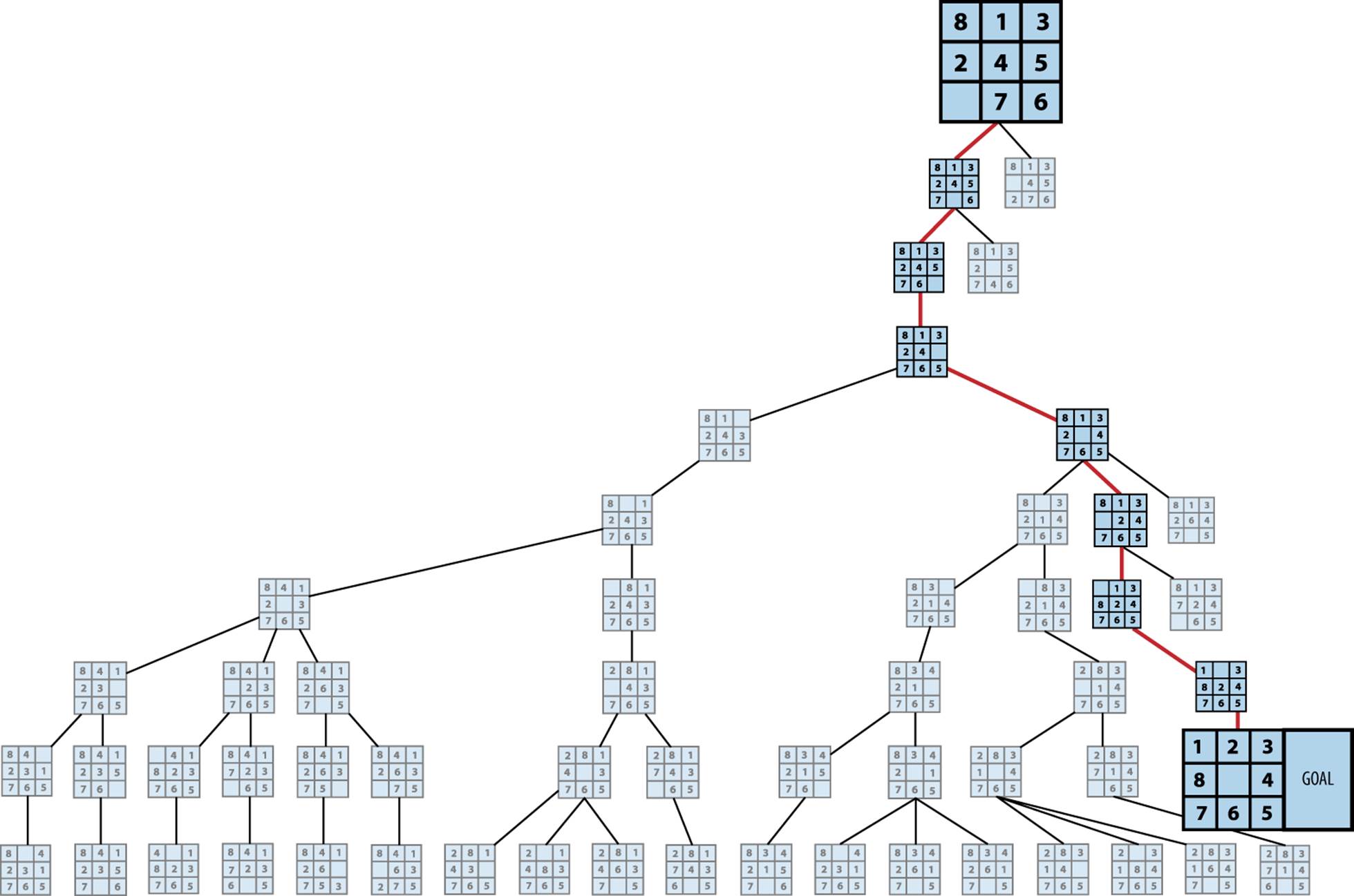
Figure 7-15. Sample Depth-First Search tree for 8-puzzle

Input/Output

The algorithm starts from an initial board state and seeks a goal state. It returns a sequence of moves that represents a path from the initial state to the goal state (or declares that no such solution was found).

Context

Depth-First Search is a blind search that is made practical by restricting the search to stop after a fixed depth bound, maxDepth, is reached, which helps manage memory resources.

Solution

Depth-First Search stores the set of open (i.e., yet to be visited) board states in a stack, and retrieves them one at a time for processing. In the implementation shown in Example 7-6, the closed set is stored in a hash table to efficiently determine when not to revisit a board state previously encountered within the search tree; the hash function used is based on the key computed for each INode object.

Each board state stores a reference, called a DepthTransition, that records (a) the move that generated it, (b) the previous state, and (c) the depth from the initial position. The algorithm generates copies of each board state, because the moves are applied directly to the boards and not undone. As soon as a node is identified as the goal, the search algorithm terminates (this is true for Breadth-First Search as well).

Example 7-6. Depth-First Search implementation

public Solution search(INode initial, INode goal) {

// If initial is the goal, return now.

if (initial.equals (goal)) { return new Solution (initial, goal); }

INodeSet open = StateStorageFactory.create (OpenStateFactory.STACK);

open.insert (initial.copy());

// states we have already visited.

INodeSet closed = StateStorageFactory.create (OpenStateFactory.HASH);

while (!open.isEmpty()) {

INode n = open.remove();

closed.insert (n);

DepthTransition trans = (DepthTransition) n.storedData();

// All successor moves translate into appended OPEN states.

DoubleLinkedList<IMove> moves = n.validMoves();

for (Iterator<IMove> it = moves.iterator(); it.hasNext(); ) {

IMove move = it.next();

// Execute move on a copy since we maintain sets of board states.

INode successor = n.copy();

move.execute (successor);

// If already visited, try another state.

if (closed.contains (successor) != null) { continue; }

int depth = 1;

if (trans != null) { depth = trans.depth+1; }

// Record previous move for solution trace. If solution, leave now,

// otherwise add to the OPEN set if still within depth bound

successor.storedData (new DepthTransition (move, n, depth));

if (successor.equals (goal)) {

return new Solution (initial, successor);

}

if (depth < depthBound) { open.insert (successor); }

}

}

return new Solution (initial, goal, false); // No solution

}

Board states are stored to avoid visiting the same state twice. We assume there is an efficient function to generate a unique key for a board state; we consider two board states to be equivalent if this function generates the same key value for the two states.

Analysis

Assume d is the maximum depth bound for Depth-First Search and define b to be the branching factor for the underlying search tree.

The performance of the algorithm is governed by problem-specific and generic characteristics. In general, the core operations provided by the open and closed sets may unexpectedly slow the algorithm down, because naïve implementations would require O(n) performance to locate a board state within the set. The key operations include:

open.remove()

Remove the next board state to evaluate.

closed.insert(INode state)

Add board state to the closed set.

closed.contains(INode state)

Determine whether board state already exists in closed.

open.insert(INode state)

Add board state into the open set, to be visited later.

Because Depth-First Search uses a stack to store the open set, remove and insert operations are performed in constant time. Because closed is a hash table that stores the board states using key values (as provided by the board state class implementing INode) the lookup time is amortized to be constant.

The problem-specific characteristics that affect the performance are (a) the number of successor board states for an individual board state, and (b) the ordering of valid moves. Some games have a large number of potential moves at each board state, which means that many depth-first paths may be ill-advised. Also, the way that moves are ordered will affect the overall search. If any heuristic information is available, make sure that moves most likely leading to a solution appear earlier in the ordered list of valid moves.

We evaluate Depth-First Search using a set of three examples (N1, N2, and N3) to show how capricious the search is with seemingly slight differences in state. In each example, 10 tiles are moved from the goal state. Occasionally Depth-First Search penetrates quickly to locate a solution. In general, the size of the search tree grows exponentially based on the branching factor b. For the 8-puzzle, the branching factor is between 2 and 4, based on where the empty tile is located, with an average of 2.67. We make the following two observations:

An ill-chosen depth level may prevent a solution from being found

For initial position N2 shown in Figure 7-16 and a depth of 25, no solution was found after searching 20,441 board states. How is this even possible? It’s because Depth-First Search will not visit the same board state twice. Specifically, the closest this particular search comes to finding the solution is on the 3,451^st board state, which is inspected in the 25^th level. That board is only three moves away from the solution! But because the board was visited just as the depth limit was reached, expansion stopped and the board was added to the closed set. If Depth-First Searchlater encountered this node again at an earlier level, it would not explore further because the node would be in the closed set.

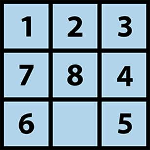
Figure 7-16. Initial position N2

It may seem better, therefore, to set the maximum depth level to be a high value; but as shown in Figure 7-17, this routinely leads to extremely large search trees and may not guarantee a solution will be found.

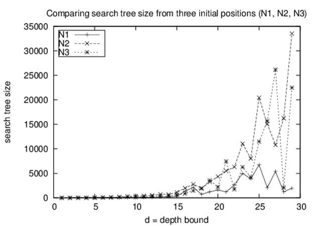
Figure 7-17. Search-tree size for Depth-First Search as depth increases

As the depth level increases, the solution found may be suboptimal

The discovered solutions grow as the depth limit increases, sometimes to two or three times larger than necessary.

Interestingly, given the example N1, an unbounded Depth-First Search actually finds a 30-move solution after processing only 30 board states, with 23 left in its open set to be processed. However, this fortunate series of events is not repeated for examples N2 and N3.

Breadth-First Search

Breadth-First Search attempts to locate a path by methodically evaluating board states closest to the initial board state. Breadth-First Search is guaranteed to find the shortest path to the goal state, if such a path exists.

The essential difference from Depth-First Search is that Breadth-First Search maintains a queue of open states that have yet to be visited, whereas Depth-First Search uses a stack. At each iteration, Breadth-First Search removes from the front of the queue an unvisited board state and expands it to compute the set of successor board states given the valid moves. If the goal state is reached, then the search terminates. Like Depth-First Search, this search makes sure not to visit the same state twice. Any successor board states that already exist within closed are discarded. The remaining unvisited board states are appended to the end of the queue of open board states, and the search continues.

Using the example from the 8-puzzle starting at Figure 7-18, the computed search tree is shown in Figure 7-19. Note how a solution is found with five moves after all paths with four moves are explored (and nearly all five-move solutions were inspected). The 20 light-gray board states in the figure are board states in the open queue waiting to be inspected. In total, 25 board states were processed.

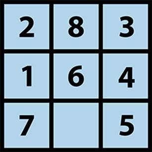
Figure 7-18. Starting board for Breadth-First Search

Input/Output

The algorithm starts from an initial board state and seeks a goal state. It returns a sequence of moves that represents a minimal-cost solution from the initial state to the goal state (or declares that no such solution was found given existing resources).

Context

A blind search is practical only if the predicted search space is within the memory space of the computer. Because Breadth-First Search methodically checks all shortest paths first, it may take quite a long time to locate paths that require a large number of moves. This algorithm may not be suitable if you need only some path from an initial state to the goal (i.e., if there is no need for it to be the shortest path).

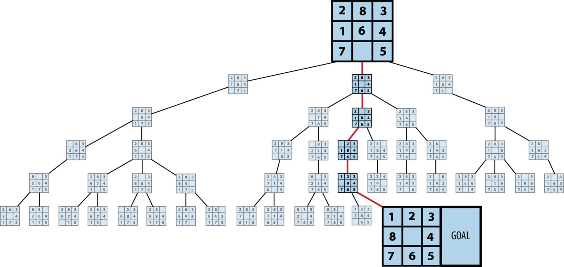
Figure 7-19. Sample Breadth-First Search tree for 8-puzzle

BREADTH-FIRST SEARCH SUMMARY

Best, Average, Worst: O(b^d)

search (initial, goal)

if initial = goal then return "Solution"

open = new Queue

closed = new Set

insert (open, copy(initial))

while open is notempty do

n = head (open)

insert (closed, n)

foreach valid move m at n do

nextState = state when playing m at n

if closed doesn't contain nextState then

if nextState = goal then return "Solution"

insert (open, nextState)

return "No Solution"

end

Breadth-First Search uses a Queue to store open states to be visited.

Remove the oldest state from the queue.

Inserting the next state will be an append operation since open is a queue.

Solution

Breadth-First Search stores the set of open (i.e., yet to be visited) board states in a queue, and retrieves them one at a time for processing. The closed set is stored using a hash table. Each board state stores a back link, called a Transition, that records the move that generated it and a reference to the previous state. Breadth-First Search generates copies of each board state, because moves are applied directly to the boards and not undone. Example 7-7 shows the implementation.

Example 7-7. Breadth-First Search implementation

public Solution search (INode initial, INode goal) {

// Return now if initial is the goal

if (initial.equals (goal)) { return new Solution (initial, goal); }

// Start from the initial state

INodeSet open = StateStorageFactory.create (StateStorageFactory.QUEUE);

open.insert (initial.copy());

// states we have already visited.

INodeSet closed = StateStorageFactory.create (StateStorageFactory.HASH);

while (!open.isEmpty()) {

INode n = open.remove();

closed.insert (n);

// All successor moves translate into appended OPEN states.

DoubleLinkedList<IMove> moves = n.validMoves();

for (Iterator<IMove> it = moves.iterator(); it.hasNext(); ) {

IMove move = it.next();

// make move on a copy

INode successor = n.copy();

move.execute (successor);

// If already visited, search this state no more

if (closed.contains (successor) != null) {

continue;

}

// Record previous move for solution trace. If solution, leave

// now, otherwise add to the OPEN set.

successor.storedData (new Transition (move, n));

if (successor.equals (goal)) {

return new Solution (initial, successor);

}

open.insert (successor);

}

}

}

Analysis

As with Depth-First Search, the algorithm’s performance is governed by problem-specific and generic characteristics. The same analysis regarding Depth-First Search applies here, and the only difference is the size of the set of open board states. Breadth-First Search must store on the order of b^d board states in open, where b is the branching factor for the board states and d is the depth of the solution found. This is much higher than Depth-First Search, which needs to store only about b*d board states in open at any one time, based on the actively pursued board state at depth d. Breadth-First Search is guaranteed to find the solution with the least number of moves that transforms the initial board state to the goal board state.

Breadth-First Search only adds a board state to the open set if it does not already exist in the closed set. You can save additional space (at the expense of some extra processing) by only adding the board state if you first confirm that it is not already contained by the open set.

A*Search

Breadth-First Search finds an optimal solution (if one exists), but it may explore a tremendous number of nodes because it makes no attempt to intelligently select the order of moves to investigate. In contrast, Depth-First Search tries to rapidly find a path by making as much progress as possible when investigating moves; however, it must be bounded because otherwise it may fruitlessly search unproductive areas of the search tree. A*Search adds heuristic intelligence to guide its search rather than blindly following either of these fixed strategies.

A*Search is an iterative, ordered search that maintains a set of open board states to explore in an attempt to reach the goal state. At each search iteration, A*Search uses an evaluation function f(n) to select a board state n from open whose f(n) has the smallest value. f(n) has the distinctive structure f(n) = g(n) + h(n), where:

§ g(n) records the length of the shortest sequence of moves from the initial state to board state n; this value is recorded as the algorithm executes

§ h(n) estimates the length of the shortest sequence of moves from n to the goal state

Thus, f(n) estimates the length of the shortest sequence of moves from initial state to goal state, passing through n. A*Search checks whether the goal state is reached only when a board state is removed from the open board states (differing from Breadth-First Search and Depth-First Search, which check when the successor board states are generated). This difference ensures the solution represents the shortest number of moves from the initial board state, as long as h(n) never overestimates the distance to the goal state.

Having a low f(n) score suggests the board state n is close to the final goal state. The most critical component of f(n) is the heuristic evaluation that computes h(n), because g(n) can be computed on the fly by recording with each board state its depth from the initial state. If h(n) is unable to accurately separate promising board states from unpromising board states, A*Search will perform no better than the blind searches already described. In particular, h(n) must be admissable—that is, it must never overstate the actual minimum cost of reaching the goal state. If the estimate is too high, A*Search may not find the optimal solution. However, it is difficult to determine an effective h(n) that is admissible and that can be computed effectively. There are numerous examples of inadmissible h(n) that still lead to solutions that are practical without necessarily being optimal.

A*SEARCH SUMMARY

Best: O(b*d) Average, Worst: O(b^d)

search (initial, goal)

initial.depth = 0

open = new PriorityQueue

closed = new Set

insert (open, copy(initial))

while open is notempty do

n = minimum (open)

insert (closed, n)

if n = goal then return "Solution"

foreach valid move m at n do

nextState = state when playing m at n

if closed contains nextState then continue

nextState.depth = n.depth + 1

prior = state in open matching nextState

if no prior state ornextState.score < prior.score then

if prior exists

remove (open, prior)

insert (open, nextState)

return "No Solution"

end

A*Search stores open states in a priority queue by evaluated score.

Must be able to rapidly locate matching node in open.

If A*Search revisits a prior state in open that now has a lower score…

…replace prior state in open with better scoring alternative.

Since open is a priority queue, nextState is inserted based on its score.

Input/Output

The algorithm starts from an initial board state in a search tree and a goal state. It assumes the existence of an evaluation function f(n) with admissible h(n) function. It returns a sequence of moves that represents the solution that most closely approximates the minimal-cost solution from the initial state to the goal state (or declares that no such solution was found given existing resources).

Context

Using the example from the 8-puzzle starting at Figure 7-20, two computed search trees are shown in Figures 7-21 and 7-22. Figure 7-21 uses the GoodEvaluator f(n) function proposed by Nilsson (1971). Figure 7-22 uses the WeakEvaluator f(n) function also proposed by Nilsson. These evaluation functions will be described shortly. The light-gray board states depict the open set when the goal is found.

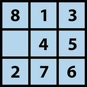
Figure 7-20. Starting board state for A*Search

Both GoodEvaluator and WeakEvaluator locate the same nine-move solution to the goal node (labeled GOAL) but GoodEvaluator is more efficient in its search. Let’s review the f(n) values associated with the nodes in both search trees to see why the WeakEvaluator search tree explores more nodes.

Observe that just two moves away from the initial state in the GoodEvaluator search tree, there is a clear path of nodes with ever-decreasing f(n) values that lead to the goal node. In contrast, the WeakEvaluator search tree explores four moves away from the initial state before narrowing its search direction. WeakEvaluator fails to differentiate board states; indeed, note how its f(n) value of the goal node is actually higher than the f(n) values of the initial node and all three of its children nodes.

Solution

A*Search stores the open board states so it can both efficiently remove the board state whose evaluation function is smallest and determine whether a specific board state exists within open. Example 7-8 contains a sample Java implementation.

Figure 7-21. Sample A*Search tree in 8-puzzle using GoodEvaluator

Figure 7-22. Sample A*Search tree in 8-puzzle using WeakEvaluator

Example 7-8. A*Search implementation

public Solution search (INode initial, INode goal) {

// Start from the initial state

int type = StateStorageFactory.PRIORITY_RETRIEVAL;

INodeSet open = StateStorageFactory.create (type);

INode copy = initial.copy();

scoringFunction.score (copy);

open.insert (copy);

// Use Hashtable to store states we have already visited.

INodeSet closed = StateStorageFactory.create (StateStorageFactory.HASH);

while (!open.isEmpty()) {

// Remove node with smallest evaluation function and mark closed.

INode best = open.remove();

// Return if goal state reached.

if (best.equals (goal)) { return new Solution (initial, best); }

closed.insert (best);

// Compute successor moves and update OPEN/CLOSED lists.

DepthTransition trans = (DepthTransition) best.storedData();

int depth = 1;

if (trans != null) { depth = trans.depth+1; }

for (IMove move : best.validMoves()) {

// Make move and score the new board state.

INode successor = best.copy();

move.execute (successor);

if (closed.contains(successor) != null) { continue; }

// Record previous move for solution trace and compute

// evaluation function to see if we have improved.

successor.storedData (new DepthTransition (move, best, depth));

scoringFunction.score (successor);

// If not yet visited, or it has better score.

INode exist = open.contains (successor);

if (exist == null || successor.score() < exist.score()) {

// remove old one, if one had existed, and insert better one

if (exist != null) {

open.remove (exist);

}

open.insert(successor);

}

}

}

// No solution.

return new Solution (initial, goal, false);

}

As with Breadth-First Search and Depth-First Search, board states are entered into the closed set when processed. Each board state stores a reference, called a DepthTransition, that records (a) the move that generated it, (b) the previous state, and (c) the depth from the initial position. That last value, the depth, is used as the g(n) component within the evaluation function. The algorithm generates copies of each board state, because the moves are applied directly to the boards and not undone.

Because A*Search incorporates heuristic information that includes a g(n) computational component, there is one situation when A*Search may review a past decision on boards already visited. A board state to be inserted into the open set may have a lower evaluation score than an identical state that already appears in open. If so, A*Search removes the existing board in open with the higher score, since that state will not be part of the minimum-cost solution. Recall the situation in Depth-First Search where board states at the depth limit were found to be (as it turned out) only three moves away from the goal state (see “Analysis”). These board states were placed into the closed set, never to be processed again. A*Search avoids this mistake by continuing to evaluate the board state in open with the lowest evaluated score.

The success of A*Search is directly dependent on its heuristic function. The h(n) component of f(n) must be carefully designed, and this effort is more of a craft than a science. If h(n) is always zero, A*Search is nothing more than Breadth-First Search. Furthermore, if h(n) overestimates the cost of reaching the goal, A*Search may not be able to find the optimal solution, although it may be possible to return some solution, assuming h(n) is not wildly off the mark. A*Search will find an optimal solution if its heuristic function h(n) is admissible.

Much of the available A*Search literature describes highly specialized h(n) functions for different domains, such as route finding on digital terrains (Wichmann and Wuensche, 2004) or project scheduling under limited resources (Hartmann, 1999). Pearl (1984) has written an extensive (and unfortunately out-of-print) reference for designing effective heuristics. Korf (2000) discusses how to design admissible h(n) functions (defined in the following section). Michalewicz and Fogel (2004) provide a recent perspective on the use of heuristics in problem solving, not just forA*Search.

For the 8-puzzle, here are three admissible heuristic functions and one badly-defined function:

FairEvaluator

P(n), where P(n) is the sum of the Manhattan distance that each tile is from its “home.”

GoodEvaluator

P(n) + 3*S(n), where P(n) is as above and S(n) is a sequence score that checks the noncentral squares in turn, allotting 0 for every tile followed by its proper successor and 2 for every tile that is not; having a piece in the center scores 1.

WeakEvaluator

Counts the number of misplaced tiles.

BadEvaluator

Total the differences of opposite cells (across the center square) and compare against the ideal of 16.

To justify why the first three heuristic functions are admissible, consider WeakEvaluator, which simply returns a count from 0 to 8. Clearly this doesn’t overestimate the number of moves but is a poor heuristic for discriminating among board states. FairEvaluator computes P(n), the Manhattan distance that computes the distance between two tiles assuming you can only move horizontally or vertically; this accurately sums the distance of each initial tile to its ultimate destination. Naturally this underestimates the actual number of moves because in 8-puzzle you can only move tiles neighboring the empty tile. What is important is not to overestimate the number of moves. GoodEvaluator adds a separate count 3*S(n) that detects sequences and adds to the move total when more tiles are out of sequence. All three of these functions are admissible.

These functions evaluated the sample board state in Figure 7-23, with the results shown in Table 7-2. You can see that all admissible functions located a shortest 13-move solution while the nonadmissible heuristic function BadEvaluator found a 19-move solution with a much larger search tree.

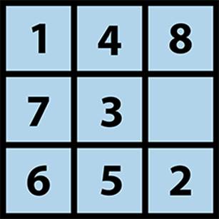
Figure 7-23. Sample board state for evaluation functions

Breadth-First Search and Depth-First Search inspect the closed set to see whether it contains a board state, so we used a hash table for efficiency. However, A*Search may need to reevaluate a board state that had previously been visited if its evaluated score function is lower than the current state. Therefore, a hash table is not appropriate because A*Search must be able to rapidly locate the board state in the open priority queue with the lowest evaluation score.

Note that Breadth-First Search and Depth-First Search retrieve the next board state from the open set in constant time because they use a queue and a stack, respectively. If we stored the open set as an ordered list, performance suffers because inserting a board state into the open set takes O(n). Nor can we use a binary heap to store the open set, because we don’t know in advance how many board states are to be evaluated. Thus, we use a balanced binary tree, which offers O(log n) performance, where n is the size of the open set, when retrieving the lowest-cost board state and for inserting nodes into the open set.

Analysis

The computational behavior of A*Search is entirely dependent on the heuristic function. Russel and Norvig (2003) summarize the characteristics of effective heuristic functions. Barr and Feigenbaum (1981) present several alternatives to consider when one cannot efficiently compute an admissible h(n) function. As the board states become more complex, heuristic functions become more important than ever—and more complicated to design. They must remain efficient to compute, or the entire search process is affected. However, even rough heuristic functions are capable of pruning the search space dramatically. For example, the 15-puzzle, the natural extension of the 8-puzzle, includes 15 tiles in a 4×4 board. It requires but a few minutes of work to create a 15-puzzle GoodEvaluator based on the logic of the 8-puzzle GoodEvaluator. With the goal state of Figure 7-24 (left) and an initial state of Figure 7-24 (right), A*Search rapidly locates a 15-move solution after processing 39 board states. When the search ends, 43 board states remain in the open set waiting to be explored.

With a 15-move limit, Depth-First Search fails to locate a solution after exploring 22,125 board states. After 172,567 board states (85,213 in the closed set and 87,354 remaining in the open set), Breadth-First Search runs out of memory when using 64MB of RAM to try the same task. Of course, you could add more memory or increase the depth limit, but this won’t work in all cases since every problem is different.

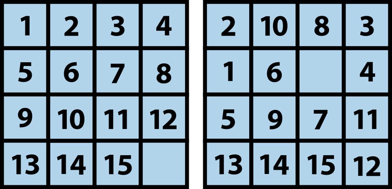
Figure 7-24. Goal for 15-puzzle (left) and sample starting board for 15-puzzle (right)

But do not be fooled by how easily A*Search solved this sample 15-puzzle; A*Search runs out of memory when attempting a more complicated initial board, such as Figure 7-25.

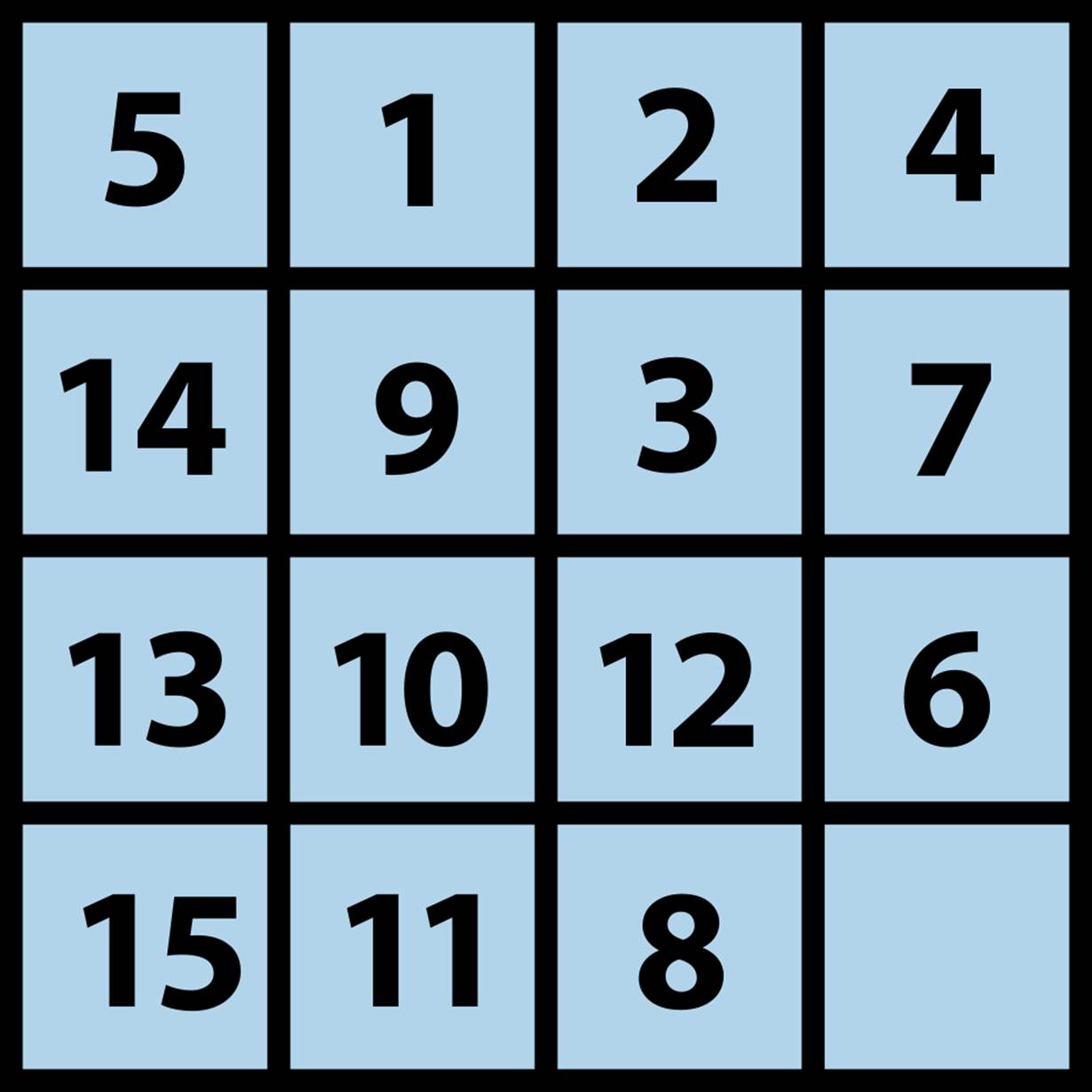
Figure 7-25. Complicated starting board for 15-puzzle

Clearly the rough evaluation function for the 15-puzzle is ineffective for the 15-puzzle, which has over 10²⁵ possible states (Korf, 2000).

Variations

Instead of only searching forward from the initial state, Kaindl and Kain (1997) augment this search by simultaneously searching backward from the goal state. Initially discarded by early AI researchers as being unworkable, Kaindl and Kainz have presented powerful arguments that the approach should be reconsidered.

A common powerful alternative to A*Search, known as IterativeDeepeningA* (or IDA*), relies on a series of expanding depth-first searches with a fixed cost bound (Reinefeld, 1993). For each successive iteration, the bound is increased based on the results of the prior iteration. IDA* is more efficient than Breadth-First Search or Depth-First Search alone because each computed cost value is based on actual move sequences rather than heuristic estimates. Korf (2000) has described how powerful heuristics, coupled with IDA*, have been used to solve random instances of the 15-puzzle, evaluating more than 400 million board states during the search.

Although A*Search produces minimal-cost solutions, the search space may be too large for A*Search to complete. The major ideas that augment A*Search and address these very large problems include:

Iterative deepening

This state search strategy uses repeated iterations of limited depth-first search, with each iteration increasing the depth limit. This approach can prioritize the nodes to be searched in successive iterations, thus reducing nonproductive searching and increasing the likelihood of rapidly converging on winning moves. Also, because the search space is fragmented into discrete intervals, real-time algorithms can search as much space as allowed within a time period and return a “best effort” result. The technique was first applied to A*Search by (Korf, 1985) to create IDA*.

Transposition tables

To avoid repeating computations that have already proved fruitless, we can hash game states and store in a transposition table the length of the path (from the source state) needed to reach each state. If the state appears later in the search, and its current depth is greater than what was discovered earlier, the search can be terminated. This approach can avoid searching entire subtrees that will ultimately prove to be unproductive.

Hierarchy

If the game state can be represented as a hierarchy, rather than as a flat model, techniques can be applied to restructure large search spaces into clusters, over which A*Search can be run. Hierarchical Path-Finding A* (HPA*) is an example of this approach (Botea et al., 2004).

Memory bound

Instead of restricting the search space by computation time, we could perform a “lossy” search and throw away various nodes as the search progresses, focusing on searches within areas that are deemed relevant. Simplified Memory Bounded A* (SMA*) is an example (Russell, 1992).

Reinefeld and Marsland (1994) summarize a variety of interesting extensions to A*Search. Much information on the use of A*Search in AI systems is available in textbooks and various online sources (Barr and Feigenbaum, 1981).

Comparing Search-Tree Algorithms

Breadth-First Search is guaranteed to find the solution with the least number of moves from the initial state, although it may evaluate a rather large number of potential move sequences as it operates. Depth-First Search tries to make as much progress as possible each time it searches, and may locate a solution rather quickly, but it also may waste a lot of time on searching parts of the search tree that seem to offer no hope for success. A*Search, when paired with an admissible heuristic function, takes the least time and finds the optimal solution, but finding an admissible function may be difficult.

It is thus worthwhile to compare Depth-First Search, Breadth-First Search, and A*Search directly. Using the 8-puzzle as our sample game, we created an initial state by randomly moving n tiles (ranging from 2 to 14); note that the same tile will not be moved twice in a row, because that would “undo” the move. Once n reached 32, the searches ran out of memory. For each board state, we execute Breadth-First Search, Depth-First Search(n), Depth-First Search(2*n), and A*Search. Note that the parameters to Depth-First Search indicate the maximum allowed depth during the search. For each move size n:

§ We total the number of board states in the open and closed lists. This reveals the efficiency of the algorithm in locating the solution. The columns marked with # contain the average of these totals over all runs. This analysis focuses on the number of states searched as the prime factor in determining search efficiency.

§ We total the number of moves in the solution once found. This reveals the efficiency of the found solution paths. The columns whose names begin with s contain the average of these totals over all runs. The number in parentheses records the number of trials that failed to locate a solution within the given ply depth.

Table 7-3 contains the aggregate results of 1,000 trials, where n random moves were made (n = 2 through 14). Table 7-3 shows two statistics: (a) the average number of states of the generated search trees, and (b) the average number of moves of the identified solutions.

Note that as n increases linearly, the size of the search tree grows exponentially for all blind approaches, but the A*Search tree remains manageable. To be precise, the growth rates of these blind searches are estimated by the following functions:

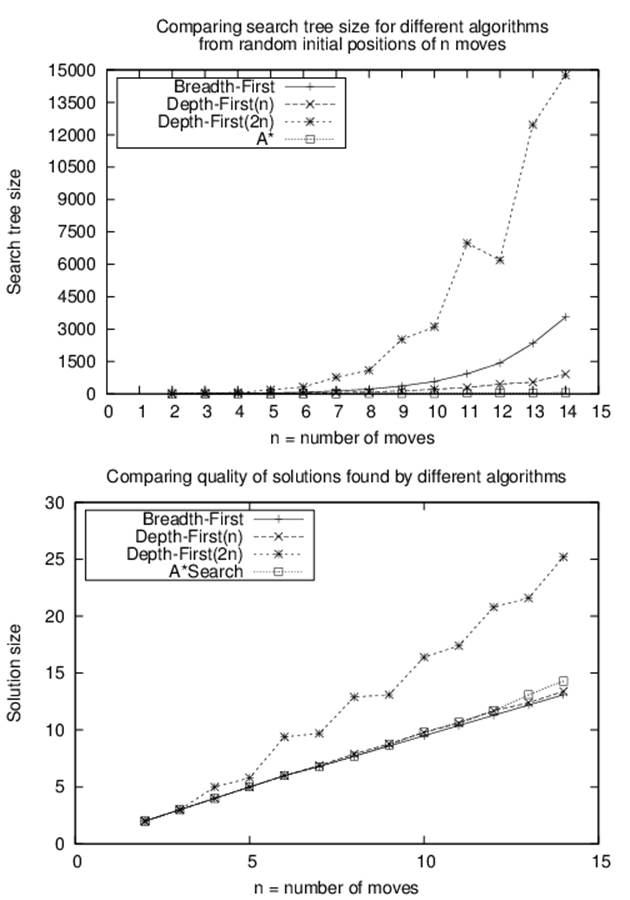
Figure 7-26. Comparing search tree size for random positions

Breadth-First Search always finds the shortest path to the solution, but note that A*Search is not far behind (because of the GoodEvaluator heuristic) even though it explores significantly fewer board states. In separate trials of A*Search with up to 30 random moves, the growth rate of the search tree was O(n^1.5147); although not linear, this size is significantly smaller than for the blind searches. The actual exponent in each of these growth rate functions is dependent on the branching factor for the problem being solved. The results of Table 7-3 are shown graphically inFigure 7-26.

Finally, note how the horizon effect prevents Depth-First Search from solving numerous cases (recall that this happens when a board state node that is only a step away from the goal is added to the closed set). In fact, in this example run of 1,000 trials, Depth-First Search failed more than 60% of the time when using a maximum depth bound of 13.

Although all three searches have the potential to explore an exponential number of states, A*Search explores the smallest number given an admissible h(n) estimation function.

There are other known ways to solve n² – 1 sliding tile puzzles besides relying on path finding. One ingenious approach proposed by Parberry (1995) is to use a Divide and Conquer strategy. That is, given an n×n puzzle, where n > 3, first complete the leftmost column and topmost row and then recursively solve the resulting (n − 1)² − 1 puzzle. When the inner problem to be solved is the 3×3 square, simply use brute force. This approach is guaranteed to find a solution that uses at most 5*n³ moves.

References

Barr, A. and E. Feigenbaum, The Handbook of Artificial Intelligence. William Kaufmann, Inc., 1981.

Berlekamp, E. and D. Wolfe, Mathematical Go: Chilling Gets the Last Point. A K Peters/CRC Press, 1994.

Botea, A., M. Müller, and J. Schaeffer, “Near optimal hierarchical path-finding,” Journal of Game Development, 1(1): 2004, http://www.cs.ualberta.ca/~mmueller/ps/hpastar.pdf.

Hartmann, S., Project Scheduling Under Limited Resources: Models, Methods, and Applications. Springer, 1999.

Kaindl, H. and G. Kainz, “Bidirectional heuristic search reconsidered,” Journal of Artificial Intelligence Research, 7: 283–317, 1997, http://arxiv.org/pdf/cs/9712102.pdf.

Korf, R. E., “Recent progress in the design and analysis of admissible heuristic functions,” Proceedings, Abstraction, Reformulation, and Approximation: 4th International Symposium (SARA), Lecture notes in Computer Science #1864: 45–51, 2000,http://www.aaai.org/Papers/AAAI/2000/AAAI00-212.pdf.

Laramée, F. D., “Chess programming Part IV: Basic search,” GameDev.net, August 26, 2000, http://www.gamedev.net/reference/articles/article1171.asp.

Michalewicz, Z. and D. Fogel, How to Solve It: Modern Heuristics. Second Edition. Springer, 2004.

Nilsson, N., Problem-Solving Methods in Artificial Intelligence. McGraw-Hill, 1971.

Parberry, I., “A real-time algorithm for the (n²−1)-Puzzle,” Information Processing Letters, 56(1):23–28, 1995, http://dx.doi.org/10.1016/0020-0190(95)00134-X.

Pearl, J., Heuristics: Intelligent Search Strategies for Computer Problem Solving. Addison-Wesley, 1984.

Pepicelli, G., “Bitwise optimization in Java: Bitfields, bitboards, and beyond,” O’Reilly on Java.com, February 2, 2005, http://www.onjava.com/pub/a/onjava/2005/02/02/bitsets.html.

Reinefeld, A., “Complete solution of the 8-puzzle and the benefit of node ordering in IDA,” Proceedings of the 13th International Joint Conference on Artificial Intelligence (IJCAI), Volume 1, 1993, http://dl.acm.org/citation.cfm?id=1624060.

Reinefeld, A. and T. Marsland, “Enhanced iterative-deepening search,” IEEE Transactions on Pattern Analysis and Machine Intelligence, 16(7): 701–710, 1994, http://dx.doi.org/10.1109/34.297950.

Russell, S. J., “Efficient memory-bounded search methods,” Proceedings, 10th European Conference on Artificial Intelligence (ECAI): 1–5, 1992.

Russell, S. J. and P. Norvig, Artificial Intelligence: A Modern Approach. Third Edition. Prentice Hall, 2009.

Samuel, A., “Some studies in machine learning using the game of checkers,” IBM Journal 3(3): 210–229, 1967, http://dx.doi.org/10.1147/rd.116.0601.

Schaeffer, J., “Game over: Black to play and draw in checkers,” Journal of the International Computer Games Association (ICGA), https://ilk.uvt.nl/icga/journal/contents/Schaeffer07-01-08.pdf.

Schaeffer, J., N. Burch, Y. Björnsson, A. Kishimoto, M. Müller, R. Lake, P. Lu, and S. Sutphen, “Checkers is solved,” Science Magazine, September 14, 2007, 317(5844):1518–1522, http://www.sciencemag.org/cgi/content/abstract/317/5844/1518.

Shannon, C., “Programming a computer for playing chess,” Philosophical Magazine, 41(314): 1950, http://tinyurl.com/ChessShannon-pdf.

Wichmann, D. and B. Wuensche, “Automated route finding on digital terrains,” Proceedings of IVCNZ, Akaroa, New Zealand, pp. 107–112, November 2004, https://www.researchgate.net/publication/245571114_Automated_Route_Finding_on_Digital_Terrains.