Algorithms in a Nutshell: A Practical Guide (2016)
Chapter 8. Network Flow Algorithms
Many problems can be presented as a network of vertices and edges, with a capacity associated with each edge over which commodities flow. The algorithms in this chapter spring from the need to solve these specific classes of problems. Ahuja (1993) contains an extensive discussion of numerous applications of network flow algorithms:
Assignment
Given a set of tasks to be carried out and a set of employees, who may cost different amounts depending on their assigned task, assign the employees to tasks while minimizing the overall expense.
Bipartite matching
Given a set of applicants who have been interviewed for a set of job openings, find a matching that maximizes the number of applicants selected for jobs for which they are qualified.
Maximum flow
Given a network that shows the potential capacity over which goods can be shipped between two locations, compute the maximum flow supported by the network.
Transportation
Determine the most cost-effective way to ship goods from a set of supplying factories to a set of retail stores.
Transshipment
Determine the most cost-effective way to ship goods from a set of supplying factories to a set of retail stores, while potentially using a set of warehouses as intermediate holding stations.
Figure 8-1 shows how each of these problems can be represented as a network flow from one or more source nodes to one or more terminal nodes. The most general definition of a problem is at the bottom, and each of the other problems is a refinement of the problem beneath it. For example, the Transportation problem is a specialized instance of the Transshipment problem because transportation graphs do not contain intermediate transshipment nodes. Thus, a program that solves Transshipment problems can be applied to Transportation problems as well.
This chapter presents the Ford–Fulkerson algorithm, which solves the Maximum Flow problem. Ford–Fulkerson can also be applied to Bipartite Matching problems, as shown in Figure 8-1. Upon further reflection, the approach outlined in Ford–Fulkerson can be generalized to solve the more powerful Minimal Cost Flow problem, which enables us to solve the Transshipment, Transportation, and Assignment problems using that algorithm.
In principle, you could apply Linear Programming (LP) to all of the problems shown in Figure 8-1, but then you would have to convert these problems into the proper LP form, whose solution would then have to be recast into the original problem (we’ll show how to do this at the end of the chapter). LP is a method to compute an optimal result (such as maximum profit or lowest cost) in a mathematical model consisting of linear relationships. In practice, however, the specialized algorithms described in this chapter outperform LP by several orders of magnitude for the problems shown in Figure 8-1.
Network Flow
We model a flow network as a directed graph G = (V, E), where V is the set of vertices and E is the set of edges over these vertices. The graph itself is connected (though not every edge need be present). A special source vertex s ∈ V produces units of a commodity that flow through the edges of the graph to be consumed by a sink vertex t ∈ V (also known as the target or terminus). A flow network assumes the supply of units produced is infinite and that the sink vertex can consume all units it receives.
Each edge (u, v) has a flow f(u, v) that defines the number of units of the commodity that flows from u to v. An edge also has a fixed capacity c(u, v) that constrains the maximum number of units that can flow over that edge. In Figure 8-2, each vertex between the source s and the sink t is numbered, and each edge is labeled as f/c, showing the flow over that edge and the maximum allowed capacity. The edge between s and v1, for example, is labeled 5/10, meaning that 5 units flow over that edge but it can sustain a capacity of up to 10. When no units are flowing over an edge (as is the case with the edge between v5 and v2), f is zero, and only the capacity is shown, outlined in a box.
Figure 8-1. Relationship between network flow problems
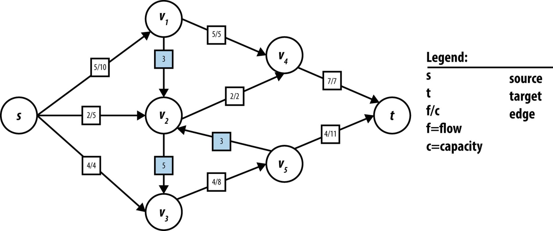
Figure 8-2. Sample flow network graph
The following criteria must be satisfied for any feasible flow f through a network:
Capacity constraint
The flow f(u, v) through an edge cannot be negative and cannot exceed the capacity of the edge c(u, v). In other words, 0 ≤ f(u, v) ≤ c(u, v). If the network does not contain an edge from u to v, we define c(u, v) to be 0.
Flow conservation
Except for the source vertex s and sink vertex t, each vertex u ∈ V must satisfy the property that the sum of f(v, u) for all edges (v, u) ∈ E (the flow into u) must equal the sum of f(u, w) for all edges (u, w) ∈ E (the flow out of u). This property ensures that flow is neither produced nor consumed in the network, except at s and t.
Skew symmetry
The quantity f(v, u) represents the opposite of the net flow from vertex u to v. This means that f(u, v) must equal –f(v, u).
In the ensuing algorithms, we refer to a network path that is a noncyclic path of unique vertices < v1, v2, …, vn > involving n-1 consecutive edges (vi, vj) in E. In the flow network shown in Figure 8-2, one possible network path is < v3, v5, v2, v4 >. In a network path, the direction of the edges can be ignored, which is necessary to properly construct augmenting paths as we will see shortly. In Figure 8-2, a possible network path is < s, v1, v4, v2, v5, t >.
Maximum Flow
Given a flow network, you can compute the maximum flow (mf) between vertices s and t given the capacity constraints c(u, v) ≥ 0 for all directed edges e = (u, v) in E. That is, compute the largest amount that can flow out of source s, through the network, and into sink t given specific capacity limits on individual edges. Starting with the lowest possible flow—a flow of 0 through every edge—Ford–Fulkerson successively locates an augmenting path through the network from s to t to which more flow can be added. The algorithm terminates when no augmenting paths can be found. The Max-flow Min-cut theorem (Ford and Fulkerson, 1962) guarantees that with non-negative integral flows and capacities, Ford–Fulkerson always terminates and identifies the maximum flow in a network.
The flow network is defined by a graph G = (V, E) with designated start vertex s and sink vertex t. Each directed edge e = (u, v) in E has a defined integer capacity c(u, v) and actual flow f(u, v). A path can be constructed from a sequence of n vertices from V, which we call p0, p1, …, pn-1, where p0 is the designated source vertex of the flow network and pn-1 is its sink vertex. The path is constructed from forward edges, where the edge over consecutive vertices (pi, pi+1) ∈ E, and backward edges, where the edge (pi+1, pi) ∈ E and the path traverses the edge opposite to its direction.
Input/Output
The flow network is defined by a graph G = (V, E) with designated start vertex s and sink vertex t. Each directed edge e = (u, v) in E has a defined integer capacity c(u, v) and actual flow f(u, v).
For each edge (u, v) in E, Ford–Fulkerson computes an integer flow f(u, v) representing the units flowing through edge (u, v). As a side effect of its termination, Ford–Fulkerson computes the min cut of the network—in other words, the set of edges that form a bottleneck, preventing further units from flowing across the network from s to t.
Solution
The implementation of Ford–Fulkerson we’ll describe here uses linked lists to store edges. Each vertex u maintains two separate lists: forward edges for the edges emanating from u and backward edges for the edges coming into u; thus each edge appears in two lists. The code repository provided with this book contains an implementation using a two-dimensional matrix to store edges, a more appropriate data structure to use for dense flow network graphs.
Ford–Fulkerson relies on the following structures:
FlowNetwork
Represents the network flow problem. This abstract class has two subclasses, one based on adjacency lists and the other using an adjacency matrix. The getEdgeStructure() method returns the underlying storage used for the edges.
VertexStructure
Maintains two linked lists (forward and backward) for the edges leaving and entering a vertex.
EdgeInfo
Records information about edges in the network flow.
VertexInfo
Records the augmenting path found by the search method. It records the previous vertex in the augmenting path and whether it was reached through a forward or backward edge.
FORD–FULKERSON SUMMARY
Best, Average, Worst: O(E*mf)
compute (G)
while exists augmenting path in G do ![]()
processPath (path)
end
processPath (path)
v = sink
delta = ∞
while v ≠ source do ![]()
u = vertex previous to v in path
if edge(u,v) is forward then
t = (u,v).capacity - (u,v).flow
else
t = (v,u).flow
delta = min (t, delta)
v = u
v = sink
while v ≠ source do ![]()
u = vertex previous to v in path
if edge(u,v) is forward then ![]()
(u,v).flow += delta
else
(v,u).flow -= delta
v = u
end
![]()
Can loop up to mf times, making overall behavior O(E*mf).
![]()
Work backward from sink to find edge with lowest potential to increase.
![]()
Adjust augmenting path accordingly.
![]()
Forward edges increase flow; backward edges reduce.
Ford–Fulkerson is implemented in Example 8-1 and illustrated in Figure 8-4. A configurable Search object computes the augmented path in the network to which additional flow can be added without violating the flow network criteria. Ford–Fulkerson makes continual progress because suboptimal decisions made in earlier iterations of the algorithm can be fixed without having to undo all past history.
Example 8-1. Sample Java Ford–Fulkerson implementation
public class FordFulkerson {
FlowNetwork network; /** Represents the FlowNetwork problem. */
Search searchMethod; /** Search method to use. */
// Construct instance to compute maximum flow across given
// network using given search method to find augmenting path.
public FordFulkerson (FlowNetwork network, Search method) {
this.network = network;
this.searchMethod = method;
}
// Compute maximal flow for the flow network. Results of the
// computation are stored within the flow network object.
public boolean compute () {
boolean augmented = false;
while (searchMethod.findAugmentingPath (network.vertices)) {
processPath (network.vertices);
augmented = true;
}
return augmented;
}
// Find edge in augmenting path with lowest potential to be increased
// and augment flows within path from source to sink by that amount.
protected void processPath (VertexInfo []vertices) {
int v = network.sinkIndex;
int delta = Integer.MAX_VALUE; // goal is to find smallest
while (v != network.sourceIndex) {
int u = vertices[v].previous;
int flow;
if (vertices[v].forward) {
// Forward edges can be adjusted by remaining capacity on edge.
flow = network.edge(u, v).capacity - network.edge(u, v).flow;
} else {
// Backward edges can be reduced only by their existing flow.
flow = network.edge(v, u).flow;
}
if (flow < delta) { delta = flow; } // smaller candidate flow.
v = u; // follow reverse path to source
}
// Adjust path (forward is added, backward is reduced) with delta.
v = network.sinkIndex;
while (v != network.sourceIndex) {
int u = vertices[v].previous;
if (vertices[v].forward) {
network.edge(u, v).flow += delta;
} else {
network.edge(v, u).flow -= delta;
}
v = u; // follow reverse path to source
}
Arrays.fill (network.vertices, null); // reset for next iteration
}
}
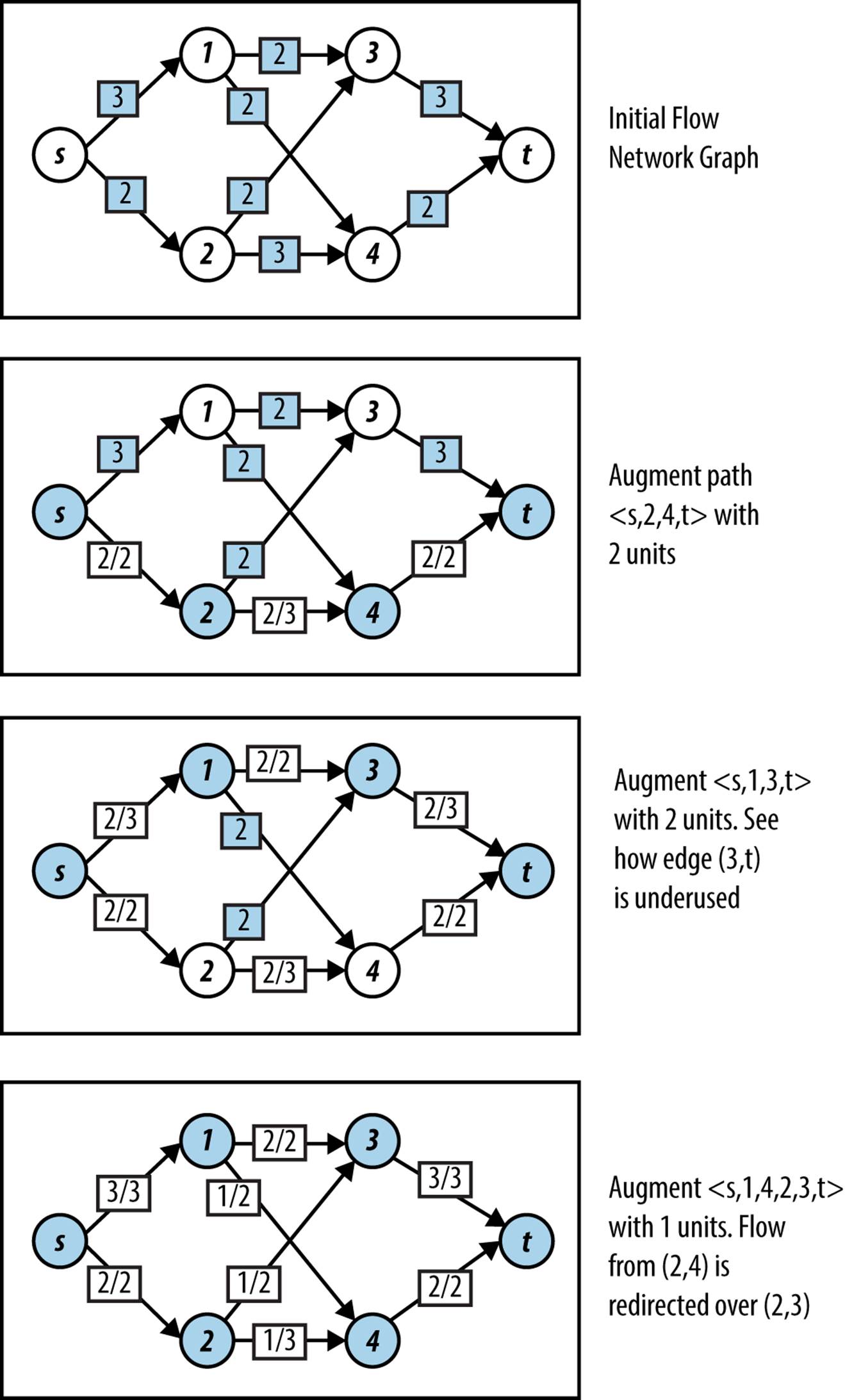
Figure 8-3. Ford–Fulkerson example
Any search method that extends the abstract Search class in Figure 8-5 can be used to locate an augmenting path. The original description of Ford–Fulkerson uses Depth-First Search while Edmonds–Karp uses Breadth-First Search (see Chapter 6).
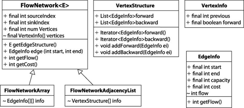
Figure 8-4. Modeling information for Ford–Fulkerson
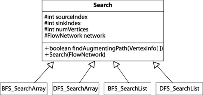
Figure 8-5. Search capability
The flow network example in Figure 8-3 shows the results of using Depth-First Search to locate an augmenting path; the implementation is listed in Example 8-2. The path structure contains a stack of vertices during its search. A potential augmenting path is extended by popping a vertexu from the stack and finding an adjacent unvisited vertex v that satisfies one of two constraints: (i) edge (u, v) is a forward edge with unfilled capacity; (ii) edge (v, u) is a backward edge with flow that can be reduced. If such a vertex is found, then v is appended to the end of path and the inner while loop continues. Eventually, the sink vertex t is visited or path becomes empty, in which case no augmenting path is possible.
Example 8-2. Using Depth-First Search to locate augmenting path
public boolean findAugmentingPath (VertexInfo[] vertices) {
// Begin potential augmenting path at source.
vertices[sourceIndex] = new VertexInfo (-1);
Stack<Integer> path = new Stack<Integer>();
path.push (sourceIndex);
// Process forward edges from u; then try backward edges.
VertexStructure struct[] = network.getEdgeStructure();
while (!path.isEmpty()) {
int u = path.pop();
// try to make forward progress first...
Iterator<EdgeInfo> it = struct[u].forward();
while (it.hasNext()) {
EdgeInfo ei = it.next();
int v = ei.end;
// not yet visited AND has unused capacity? Plan to increase.
if (vertices[v] == null && ei.capacity > ei.flow) {
vertices[v] = new VertexInfo (u, FORWARD);
if (v == sinkIndex) { return true; } // we have found one!
path.push (v);
}
}
// try backward edges
it = struct[u].backward();
while (it.hasNext()) {
// try to find an incoming edge into u whose flow can be reduced.
EdgeInfo rei = it.next();
int v = rei.start;
// now try backward edge not yet visited (can't be sink!)
if (vertices[v] == null && rei.flow > 0) {
vertices[v] = new VertexInfo (u, BACKWARD);
path.push (v);
}
}
}
return false; // nothing
}
As the path is expanded, the vertices array stores VertexInfo information about forward and backward edges enable the augmenting path to be traversed within the processPath method from Example 8-1.
The implementation of the Breadth-First Search alternative, known as Edmonds–Karp, is shown in Example 8-3. Here the path structure contains a queue of vertices during its search. The potential augmenting path is expanded by removing a vertex u from the head of the queue and expanding the queue by appending adjacent unvisited vertices through which the augmented path may exist. Again, either the sink vertex t will be visited or path becomes empty (in which case no augmenting path is possible). Given the same example flow network from Figure 8-3, the four augmenting paths located using Breadth-First Search are < s, 1, 3, t >, < s, 1, 4, t >, < s, 2, 3, t >, and < s, 2, 4, t >. The resulting maximum flow will be the same.
Example 8-3. Using Breadth-First Search to locate augmenting path
public boolean findAugmentingPath (VertexInfo []vertices) {
// Begin potential augmenting path at source with maximum flow.
vertices[sourceIndex] = new VertexInfo (-1);
DoubleLinkedList<Integer> path = new DoubleLinkedList<Integer>();
path.insert (sourceIndex);
// Process forward edges out of u; then try backward edges into u.
VertexStructure struct[] = network.getEdgeStructure();
while (!path.isEmpty()) {
int u = path.removeFirst();
Iterator<EdgeInfo> it = struct[u].forward(); // edges out from u
while (it.hasNext()) {
EdgeInfo ei = it.next();
int v = ei.end;
// if not yet visited AND has unused capacity? Plan to increase.
if (vertices[v] == null && ei.capacity > ei.flow) {
vertices[v] = new VertexInfo (u, FORWARD);
if (v == sinkIndex) { return true; } // path is complete.
path.insert (v); // otherwise append to queue
}
}
it = struct[u].backward(); // edges into u
while (it.hasNext()) {
// try to find an incoming edge into u whose flow can be reduced.
EdgeInfo rei = it.next();
int v = rei.start;
// Not yet visited (can't be sink!) AND has flow to be decreased?
if (vertices[v] == null && rei.flow > 0) {
vertices[v] = new VertexInfo (u, BACKWARD);
path.insert (v); // append to queue
}
}
}
return false; // no augmented path located.
}
When Ford–Fulkerson terminates, the vertices in V can be split into two disjoint sets, S and T (where T = V – S). Note that s ∈ S, whereas t ∈ T. S is computed to be the set of vertices from V that were visited in the final failed attempt to locate an augmenting path. The importance of these sets is that the forward edges between S and T comprise a min cut or a bottleneck in the flow network. That is, the capacity that can flow from S to T is minimized, and the available flow between S and T is already at full capacity.
Analysis
Ford–Fulkerson terminates because the units of flow are non-negative integers (Ford–Fulkerson, 1962). The performance of Ford–Fulkerson using Depth-First Search is O(E*mf) and is based on the final value of the maximum flow, mf. Briefly, it is possible that each iteration adds only one unit of flow to the augmenting path, and thus networks with very large capacities might require a great number of iterations. It is striking that the running time is based not on the problem size (i.e., the number of vertices or edges) but on the capacities of the edges themselves.
When using Breadth-First Search (identified by name as the Edmonds–Karp variation), the performance is O(V*E2). Breadth-First Search finds the shortest augmented path in O(V + E), which is really O(E) because the number of vertices is smaller than the number of edges in the connected flow network graph. Cormen et al. (2009) prove that the number of flow augmentations performed is on the order of O(V*E), leading to the final result that Edmonds–Karp has O(V*E2) performance. Edmonds–Karp often outperforms Ford–Fulkerson by relying on Breadth-First Search to pursue all potential paths in order of length, rather than potentially wasting much effort in a depth-first “race” to the sink.
Optimization
Typical implementations of network-flow problems use arrays to store information. We choose instead to present each algorithm with lists because the code is more readable and readers can understand how the algorithm works. It is worth considering, however, how much performance speedup can be achieved by optimizing the resulting code; in Chapter 2 we showed a 50% performance improvement in optimizing the multiplication of n-digit numbers. It is clear that faster code can be written, but it may not be easy to understand or maintain if the problem changes. With this caution in mind, Example 8-4 contains an optimized Java implementation of Ford–Fulkerson.
Example 8-4. Optimized Ford–Fulkerson implementation
public class Optimized extends FlowNetwork {
int[][] capacity; // Contains all capacities.
int[][] flow; // Contains all flows.
int[] previous; // Contains predecessor information of path.
int[] visited; // Visited during augmenting path search.
final int QUEUE_SIZE; // Size of queue will never be greater than n.
final int queue[]; // Use circular queue in implementation.
// Load up the information
public Optimized (int n, int s, int t, Iterator<EdgeInfo> edges) {
super (n, s, t);
queue = new int[n];
QUEUE_SIZE = n;
capacity = new int[n][n];
flow = new int[n][n];
previous = new int[n];
visited = new int [n];
// Initially, flow is set to 0. Pull info from input.
while (edges.hasNext()) {
EdgeInfo ei = edges.next();
capacity[ei.start][ei.end] = ei.capacity;
}
}
// Compute and return the maxFlow.
public int compute (int source, int sink) {
int maxFlow = 0;
while (search(source, sink)) { maxFlow += processPath (source, sink); }
return maxFlow;
}
// Augment flow within network along path found from source to sink.
protected int processPath (int source, int sink) {
// Determine amount by which to increment the flow. Equal to
// minimum over the computed path from sink to source.
int increment = Integer.MAX_VALUE;
int v = sink;
while (previous[v] != −1) {
int unit = capacity[previous[v]][v] - flow[previous[v]][v];
if (unit < increment) { increment = unit; }
v = previous[v];
}
// push minimal increment over the path
v = sink;
while (previous[v] != −1) {
flow[previous[v]][v] += increment; // forward edges.
flow[v][previous[v]] -= increment; // don't forget back edges
v = previous[v];
}
return increment;
}
// Locate augmenting path in the Flow Network from source to sink.
public boolean search (int source, int sink) {
// clear visiting status. 0=clear, 1=actively in queue, 2=visited
for (int i = 0 ; i < numVertices; i++) { visited[i] = 0; }
// create circular queue to process search elements.
queue[0] = source;
int head = 0, tail = 1;
previous[source] = −1; // make sure we terminate here.
visited[source] = 1; // actively in queue.
while (head != tail) {
int u = queue[head]; head = (head + 1) % QUEUE_SIZE;
visited[u] = 2;
// add to queue unvisited neighbors of u with enough capacity.
for (int v = 0; v < numVertices; v++) {
if (visited[v] == 0 && capacity[u][v] > flow[u][v]) {
queue[tail] = v;
tail = (tail + 1) % QUEUE_SIZE;
visited[v] = 1; // actively in queue.
previous[v] = u;
}
}
}
return visited[sink] != 0; // did we make it to the sink?
}
}
Related Algorithms
The Push/Relabel algorithm introduced by Goldberg and Tarjan (1986) improves the performance to O(V*E*log(V2/E)) and also provides an algorithm that can be parallelized for greater gains. A variant of the problem, known as the Multi-Commodity Flow problem, generalizes the Maximum Flow problem stated here. Briefly, instead of having a single source and sink, consider a shared network used by multiple sources si and sinks ti to transmit different commodities. The capacity of the edges is fixed, but the usage demanded for each source and sink may vary. Practical applications of algorithms that solve this problem include routing in wireless networks (Fragouli and Tabet, 2006). Leighton and Rao (1999) have written a widely cited reference for multicommodity problems.
There are several slight variations to the Maximum Flow problem:
Vertex capacities
What if a flow network places a maximum capacity k(v) flowing through a vertex v in the graph? We can solve these problems by constructing a modified flow network Gm as follows. For each vertex v in G, create two vertices va and vb. Create edge (va, vb) with a flow capacity of k(v). For each incoming edge (u, v) in G with capacity c(u, v), create a new edge (u, va) with capacity c(u, v). For each outgoing edge (v, w) in G, create edge (vb, w) in Gm with capacity k(v). A solution in Gm determines the solution to G.
Undirected edges
What if the flow network G has undirected edges? Construct a modified flow network Gm with the same set of vertices. For each edge (u, v) in G with capacity c(u, v), construct a pair of edges (u, v) and (v, u) each with the same capacity c(u, v). A solution in Gm determines the solution toG.
Bipartite Matching
Matching problems exist in numerous forms. Consider the following scenario. Five applicants have been interviewed for five job openings. The applicants have listed the jobs for which they are qualified. The task is to match applicants to jobs such that each job opening is assigned to exactly one qualified applicant.
We can use Ford–Fulkerson to solve the Bipartite Matching problem. This technique is known in computer science as “problem reduction.” We reduce the Bipartite Matching problem to a Maximum Flow problem in a flow network by showing (a) how to map the Bipartite Matching problem input into the input for a Maximum Flow problem, and (b) how to map the output of the Maximum Flow problem into the output of the Bipartite Matching problem.
Input/Output
A Bipartite Matching problem consists of a set of n elements, where si ∈ S; a set of m partners, where tj ∈ T; and a set of p acceptable pairs, where pk ∈ P. Each P pair associates an element si ∈ S with a partner tj ∈ T. The sets S and T are disjoint, which gives this problem its name.
The output is a set of (si, tj) pairs selected from the original set of acceptable pairs, P. These pairs represent a maximum number of pairs allowed by the matching. The algorithm guarantees that no greater number of pairs can be matched (although there may be other arrangements that lead to the same number of pairs).
Solution
Instead of devising a new algorithm to solve this problem, we reduce a Bipartite Matching problem instance into a Maximum Flow instance. In Bipartite Matching, selecting the match (si, tj) for element si ∈ S with partner tj ∈ T prevents either si or tj from being selected again in another pairing. Let n be the size of S and m be the size of T. To produce this same behavior in a flow network graph, construct G = (V, E):
V contains n + m + 2 vertices
Each element si maps to a vertex numbered i. Each partner tj maps to a vertex numbered n + j. Create a new source vertex src (labeled 0) and a new target vertex tgt (labeled n + m + 1).
E contains n + m + k edges
There are n edges connecting the new src vertex to the vertices mapped from S. There are m edges connecting the new tgt vertex to the vertices mapped from T. For each of the k pairs, pk = (si, tj), add edge (i, n + j). All of these edges must have a flow capacity of 1.
Computing the Maximum Flow in the flow network graph G produces a maximal matching set for the original Bipartite Matching problem, as proven in Cormen et al. (2009). For an example, consider Figure 8-6(a), where it is suggested that the two pairs (a, z) and (b, y) form the maximum number of pairs; the corresponding flow network using this construction is shown in Figure 8-6(b), where vertex 1 corresponds to a, vertex 4 corresponds to x, and so on. Upon reflection we can improve this solution to select three pairs, (a, z), (c, y), and (b, x). The corresponding adjustment to the flow network is made by finding the augmenting path <0,3,5,2,4,7>. Applying this augmenting path removes match (b, y) and adds match (b, x) and (c, y).
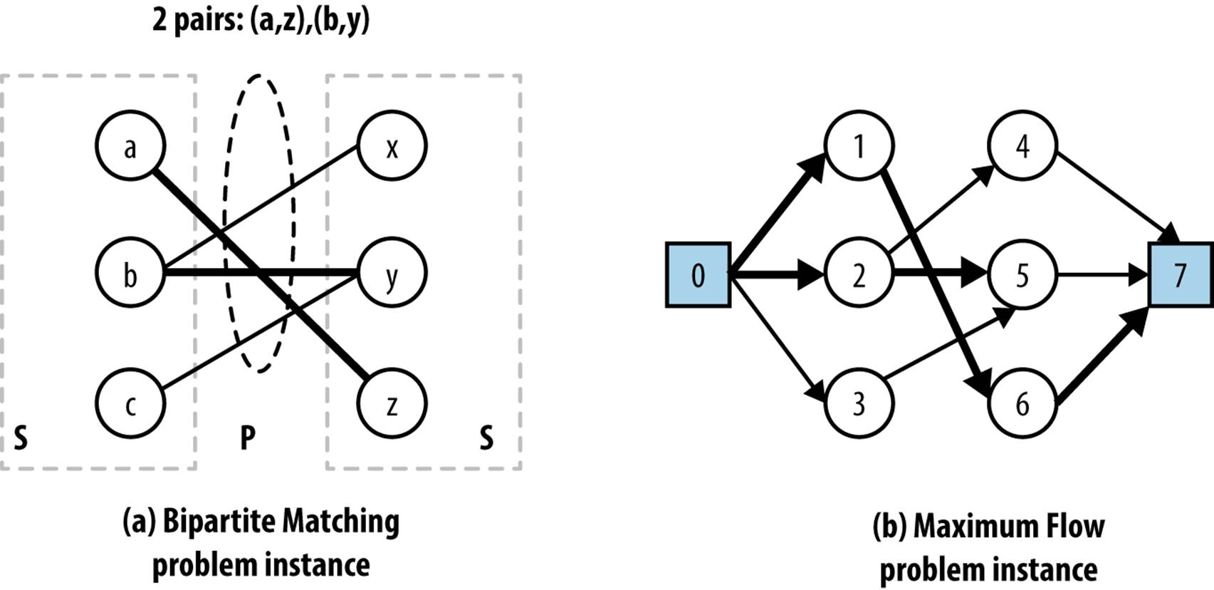
Figure 8-6. Bipartite Matching reduces to Maximum Flow
Once the Maximum Flow is determined, we convert the output of the Maximum Flow problem into the appropriate output for the Bipartite Matching problem. That is, for every edge (si, tj) whose flow is 1, indicate that the pairing (si, tj) ∈ P is selected. In the code shown in Example 8-5, error checking has been removed to simplify the presentation.
Example 8-5. Bipartite Matching using Ford–Fulkerson
public class BipartiteMatching {
ArrayList<EdgeInfo> edges; /* Edges for S and T. */
int ctr = 0; /* Unique id counter. */
/* Maps that convert between problem instances. */
Hashtable<Object,Integer> map = new Hashtable<Object,Integer>();
Hashtable<Integer,Object> reverse = new Hashtable<Integer,Object>();
int srcIndex; /* Source index of flow network problem. */
int tgtIndex; /* Target index of flow network problem. */
int numVertices; /* Number of vertices in flow network problem. */
public BipartiteMatching (Object[] S, Object[] T, Object[][] pairs) {
edges = new ArrayList<EdgeInfo>();
// Convert pairs into input for FlowNetwork with capacity 1.
for (int i = 0; i < pairs.length; i++) {
Integer src = map.get (pairs[i][0]);
Integer tgt = map.get (pairs[i][1]);
if (src == null) {
map.put (pairs[i][0], src = ++ctr);
reverse.put (src, pairs[i][0]);
}
if (tgt == null) {
map.put (pairs[i][1], tgt = ++ctr);
reverse.put (tgt, pairs[i][1]);
}
edges.add (new EdgeInfo (src, tgt, 1));
}
// add extra "source" and extra "target" vertices
srcIndex = 0;
tgtIndex = S.length + T.length+1;
numVertices = tgtIndex+1;
for (Object o : S) {
edges.add (new EdgeInfo (0, map.get (o), 1));
}
for (Object o : T) {
edges.add (new EdgeInfo (map.get (o), tgtIndex, 1));
}
}
public Iterator<Pair> compute() {
FlowNetworkArray network = new FlowNetworkArray (numVertices,
srcIndex, tgtIndex, edges.iterator());
FordFulkerson solver = new FordFulkerson (network,
new DFS_SearchArray(network));
solver.compute();
// retrieve from original edgeInfo set; ignore created edges to the
// added "source" and "target". Only include in solution if flow == 1
ArrayList<Pair> pairs = new ArrayList<Pair>();
for (EdgeInfo ei : edges) {
if (ei.start != srcIndex && ei.end != tgtIndex) {
if (ei.getFlow() == 1) {
pairs.add (new Pair (reverse.get (ei.start),
reverse.get (ei.end)));
}
}
}
return pairs.iterator(); // iterator generates solution
}
}
Analysis
For a problem reduction to be efficient, it must be possible to efficiently map both the problem instance and the computed solutions. The Bipartite Matching problem M = (S, T, P) is converted into a graph G = (V, E) in n + m + k steps. The resulting graph G has n + m + 2 vertices and n + m +k edges, and thus the size of the graph is only a constant size larger than the original Bipartite Matching problem size. This important feature of the construction ensures we have an efficient solution to the Bipartite Matching problem. After Ford–Fulkerson computes the maximum flow, the edges in the network with a flow of 1 correspond to pairs in the Bipartite Matching problem that belong to the matching. Determining these edges requires k steps, or O(k) extra processing, to “read” the solution to Bipartite Matching.
Reflections on Augmenting Paths
The Maximum Flow problem underlies solutions to all the remaining problems discussed earlier in this chapter in Figure 8-1. Each requires steps to represent it as a flow network, after which we can minimize the cost of that flow. If we associate with each edge (u, v) in the network a costd(u, v) that reflects the per-unit cost of shipping a unit over edge (u, v), the goal is to minimize
Σ f(u, v)*d(u, v)
for all edges in the flow network. Now, for Ford–Fulkerson, we stressed the importance of finding an augmenting path that could increase the maximum flow through the network. But what if we modify the search routine to find the least costly augmentation, if one exists? We have already seen Greedy algorithms (such as Prim’s Algorithm for building a Minimum Spanning Tree in Chapter 6) that iteratively select the least costly extension; perhaps such an approach will work here.
To find the least costly augmentation path, we cannot rely strictly on a breadth-first or a depth-first approach. As we saw with Prim’s Algorithm, we must use a priority queue to store and compute the distance of each vertex in the flow network from the source vertex. We essentially compute the costs of shipping an additional unit from the source vertex to each vertex in the network, and we maintain a priority queue based on the ongoing computation:
1. As the search proceeds, the priority queue stores the ordered set of nodes that define the active searching focus.
2. To expand the search, retrieve from the priority queue the vertex u whose distance (in terms of cost) from the source is the smallest. Then locate a neighboring vertex v that has not yet been visited and that meets one of two conditions: either (a) the forward edge (u, v) still has remaining capacity to be increased, or (b) the backward edge (v, u) has flow that can be reduced.
3. If the sink index is encountered during the exploration, the search terminates successfully with an augmenting path; otherwise, no such augmenting path exists.
The Java implementation of ShortestPathArray is shown in Example 8-6. When this method returns true, the vertices parameter contains information about the augmenting path.
Example 8-6. Shortest path (in costs) search for Ford–Fulkerson
public boolean findAugmentingPath (VertexInfo[] vertices) {
Arrays.fill (vertices, null); // reset for iteration
// Construct queue using BinaryHeap. The inqueue[] array avoids
// an O(n) search to determine if an element is in the queue.
int n = vertices.length;
BinaryHeap<Integer> pq = new BinaryHeap<Integer> (n);
boolean inqueue[] = new boolean [n];
// initialize dist[] array. Use INT_MAX when edge doesn't exist.
for (int u = 0; u < n; u++) {
if (u == sourceIndex) {
dist[u] = 0;
pq.insert (sourceIndex, 0);
inqueue[u] = true;
} else {
dist[u] = Integer.MAX_VALUE;
}
}
while (!pq.isEmpty()) {
int u = pq.smallestID();
inqueue[u] = false;
// When reach sinkIndex we are done.
if (u == sinkIndex) { break; }
for (int v = 0; v < n; v++) {
if (v == sourceIndex || v == u) continue;
// forward edge with remaining capacity if cost is better.
EdgeInfo cei = info[u][v];
if (cei != null && cei.flow < cei.capacity) {
int newDist = dist[u] + cei.cost;
if (0 <= newDist && newDist < dist[v]) {
vertices[v] = new VertexInfo (u, Search.FORWARD);
dist[v] = newDist;
if (inqueue[v]) {
pq.decreaseKey (v, newDist);
} else {
pq.insert (v, newDist);
inqueue[v] = true;
}
}
}
// backward edge with at least some flow if cost is better.
cei = info[v][u];
if (cei != null && cei.flow > 0) {
int newDist = dist[u] - cei.cost;
if (0 <= newDist && newDist < dist[v]) {
vertices[v] = new VertexInfo (u, Search.BACKWARD);
dist[v] = newDist;
if (inqueue[v]) {
pq.decreaseKey (v, newDist);
} else {
pq.insert (v, newDist);
inqueue[v] = true;
}
}
}
}
}
return dist[sinkIndex] != Integer.MAX_VALUE;
}
Armed with this strategy for locating the lowest-cost augmenting path, we can solve the remaining problems shown in Figure 8-1. To show the effect of this low-cost search strategy, Figure 8-7 illustrates the side-by-side computation on a small example comparing a straightforward Maximum Flow computation with a Minimum Cost Flow computation. Each iteration moving vertically down the figure is another pass through the while loop within the compute() method of Ford–Fulkerson (as seen in Figure 8-1). The result, at the bottom of the figure, is the maximum flow found by each approach.
In this example, you are the shipping manager in charge of two factories in Chicago (v1) and Washington, D.C. (v2) that can each produce 300 widgets daily. You must ensure that two customers in Houston (v3) and Boston (v4) each receive 300 widgets a day. You have several options for shipping, as shown in the figure. For example, between Washington, D.C. and Houston, you may ship up to 280 widgets daily at $4 per widget, but the cost increases to $6 per widget if you ship from Washington, D.C. to Boston (although you can then send up to 350 widgets per day along that route).
Figure 8-7. Side-by-side computation showing difference when considering the minimum cost flow
It may not even be clear that Ford–Fulkerson can be used to solve this problem, but note that we can create a graph G with a new source vertex s0 that connects to the two factory nodes (v1 and v2), and the two customers (v3 and v4) connect to a new sink vertex t5. To save space, the source and sink vertices s0 and t5 are omitted. On the lefthand side of Figure 8-7 we execute the Edmonds–Karp variation to demonstrate that we can meet all of our customer needs as requested, at the total daily shipping cost of $3,600. During each of the four iterations by Ford–Fulkerson, the impact of the augmented path is shown (when an iteration updates the flow for an edge, the flow value is shaded gray).
Is this the lowest cost we can achieve? The righthand side of Figure 8-7 shows the execution of Ford–Fulkerson using ShortestPathArray as its search strategy, as described in Example 8-6. Note how the first augmented path found takes advantage of the lowest-cost shipping rate. AlsoShortestPathArray only uses the costliest shipping route from Chicago (v1) to Houston (v3) when there is no other way to meet the customer needs; when this happens, the augmented path reduces the existing flows between Washington, D.C. (v2) and Houston (v3), as well as between Washington, D.C. (v2) and Boston (v4).
Minimum Cost Flow
To solve a Minimum Cost Flow problem we need only construct a flow network graph and ensure it satisfies the criteria discussed earlier—capacity constraint, flow conservation, and skew symmetry—as well as two additional criteria, supply satisfaction and demand satisfaction. These terms came into being when the problem was defined in an economic context, and they roughly correspond to the electical engineering concepts of a source and a sink:
Supply satisfaction
For each source vertex si ∈ S, the sum of f(si, v) for all edges (si, v) ∈ E (the flow out of si) minus the sum of f(u, si) for all edges (u, si) ∈ E (the flow into si) must be less than or equal to sup(si). That is, the supply sup(si) at each source vertex is a firm upper bound on the net flow from that vertex.
Demand satisfaction
For each sink vertex tj ∈ T, the sum of f(u, tj) for all edges (u, tj) ∈ E (the flow into tj) minus the sum of f(tj, v) for all edges (tj, v) ∈ E (the flow out of tj) must be less than or equal to dem(tj). That is, the dem(tj) at each target vertex is a firm upper bound on the net flow into that vertex.
To simplify the algorithmic solution, we further constrain the flow network graph to have a single source vertex and sink vertex. This can be easily accomplished by taking an existing flow network graph with any number of source and sink vertices and adding two new vertices. First, add a new vertex (which we refer to as s0) to be the source vertex for the flow network graph, and add edges (s0, si) for all si ∈ S whose capacity c(s0, si) = sup(si) and whose cost d(s0, si) = 0. Second, add a new vertex (referred to as tgt, for target) to be the sink vertex for the flow network graph, and add edges (tj, tgt) for all tj ∈ T whose capacity c(tj, tgt) = dem(tj) and whose cost d(t0, tj) = 0. As you can see, adding these vertices and edges does not increase the cost of the network flow, nor do they reduce or increase the final computed flow over the network.
The supplies sup(si), demands dem(tj), and capacities c(u, v) are all greater than 0. The shipping cost d(u, v) associated with each edge may be greater than or equal to zero. When the resulting flow is computed, all f(u, v) values will be greater than or equal to zero.
We now present the constructions that allow us to solve each of the remaining flow network problems listed in Figure 8-1. For each problem, we describe how to reduce the problem to Minimum Cost Flow.
Transshipment
The inputs are:
§ m supply stations si, each capable of producing sup(si) units of a commodity
§ n demand stations tj, each demanding dem(tj) units of the commodity
§ w warehouse stations wk, each capable of receiving and reshipping (known as “transshipping”) a maximum maxk units of the commodity at the fixed warehouse processing cost of wpk per unit
There is a fixed shipping cost of d(i, j) for each unit shipping from supply station si to demand stations tj, a fixed transshipping cost of ts(i, k) for each unit shipped from supply station si to warehouse station wk, and a fixed transshipping cost of ts(k, j) for each unit shipped from warehouse station wk to demand station tj. The goal is to determine the flow f(i, j) of units from supply station si to demand station tj that minimizes the overall total cost, which can be concisely defined as:
Total Cost (TC) = Total Shipping Cost (TSC) + Total Transshipping Cost (TTC)
TSC = Σi Σj d(i, j)*f(i, j)
TTC = Σi Σk ts(i, k)*f(i, k) + Σj Σk ts(j, k)*f(j, k)
The goal is to find integer values for f(i, j) ≥ 0 that ensure that TC is a minimum while meeting all of the supply and demand constraints. Finally, the net flow of units through a warehouse must be zero, to ensure no units are lost (or added). The supplies sup(si) and demands dem(ti) are all greater than 0. The shipping costs d(i, j), ts(i, k), and ts(k, j) may be greater than or equal to zero.
Solution
We convert the Transshipment problem instance into a Minimum Cost Flow problem instance (as illustrated in Figure 8-8) by constructing a graph G = (V, E) such that:
V contains n + m + 2*w + 2 vertices
Each supply station si maps to a vertex numbered i. Each warehouse wk maps to two different vertices, one numbered m + 2*k − 1 and one numbered m + 2*k. Each demand station tj maps to 1 + m + 2*w + j. Create a new source vertex src (labeled 0) and a new target vertex tgt (labeled n+ m + 2*w + 1).
E contains (w + 1)*(m + n) + m*n + w edges
The Transshipment class in the code repository encodes the process for constructing edges for the Transshipment problem instance.
Briefly, the artificial source vertex is connected to the m supply vertices, with zero cost and capacity equal to the supplier capacity sup(si). These m supply vertices are each connected to the n demand vertices with cost equal to d(i, j) and infinite capacity. The n demand vertices are connected to the new artificial target vertex with zero cost and capacity equal to dem(tj). There are w warehouse nodes, each connected to the m supply vertices with cost equal to ts(i, k) and capacity equal to the supplier capacity sup(si); these warehouse nodes are also connected to the n demand vertices with cost equal to ts(k, j) and capacity equal to the demand capacity dem(tj). Finally, edges between warehouses have capacities and costs based on the warehouse limits and costs.
Once the Minimum Cost Flow solution is available, the transshipment schedule can be constructed by locating those edges (u, v) ∈ E whose f(u, v) > 0. The cost of the schedule is the sum total of f(u, v)*d(u, v) for these edges.
Transportation
The Transportation problem is simpler than the Transshipment problem because there are no intermediate warehouse nodes. The inputs are:
§ m supply stations si, each capable of producing sup(si) units of a commodity
§ n demand stations tj, each demanding dem(tj) units of the commodity
There is a fixed per-unit cost d(i, j) ≥ 0 associated with transporting a unit over the edge (i, j). The goal is to determine the flow f(i, j) of units from supply stations si to demand stations tj that minimizes the overall transportation cost, TSC, which can be concisely defined as:
Total Shipping Cost (TSC) = Σi Σj d(i, j)*f(i, j)
The solution must also satisfy both the total demand for each demand station tj and the supply capabilities for supply stations si.
Figure 8-8. Sample Transshipment problem instance converted to Minimum Cost Flow problem instance
Solution
We convert the Transportation problem instance into a Transshipment problem instance with no intermediate warehouse nodes.
Assignment
The Assignment problem is simply a more restricted version of the Transportation problem: each supply node must supply only a single unit, and the demand for each demand node is also one.
Solution
We convert the Assignment problem instance into a Transportation problem instance, with the restriction that the supply nodes provide a single unit and the demand nodes require a single unit.
Linear Programming
The different problems described in this chapter can all be solved using Linear Programming (LP), a powerful technique that optimizes a linear objective function, subject to linear equality and inequality constraints (Bazaraa and Jarvis, 1977).
To show LP in action, we convert the Transportation problem depicted in Figure 8-8 into a series of linear equations to be solved by an LP solver. We use a general-purpose commercial mathematics software package known as Maple to carry out the computations. As you recall, the goal is to maximize the flow over the network while minimizing the cost. We associate a variable with the flow over each edge in the network; thus the variable e13 represents f(1,3). The function to be minimized is Cost, which is defined as the sum total of the shipping costs over each of the four edges in the network. This cost equation has the same constraints we described earlier for network flows:
Flow conservation
The sum total of the edges emanating from a source vertex must equal its supply. The sum total of the edges entering a demand vertex must be equal to its demand.
Capacity constraint
The flow over an edge f(i, j) must be greater than or equal to zero. Also, f(i, j) ≤ c(i, j).
When executing the Maple solver, the computed result is {e13 = 100, e24 = 100, e23 = 200, e14 = 200}, which corresponds exactly to the minimum cost solution of 3,300 found earlier (see Example 8-7).
Example 8-7. Maple commands to apply minimization to Transportation problem
Constraints := [
# conservation of units at each node
e13+e14 = 300, # CHI
e23+e24 = 300, # DC
e13+e23 = 300, # HOU
e14+e24 = 300, # BOS
# maximum flow on individual edges
0 <= e13, e13 <= 200,
0 <= e14, e14 <= 200,
0 <= e23, e23 <= 280,
0 <= e24, e24 <= 350
];
Cost := 7*e13 + 6*e14 + 4*e23 + 6*e24;
# Invoke linear programming to solve problem
minimize (Cost, Constraints, NONNEGATIVE);
The Simplex algorithm designed by George Dantzig in 1947 makes it possible to solve problems such as those shown in Example 8-7, which involve hundreds or thousands of variables (McCall, 1982). Simplex has repeatedly been shown to be efficient in practice, although the approach can, under unfortunate circumstances, lead to an exponential number of computations. It is not recommended that you implement the Simplex algorithm yourself, both because of its complexity and because there are commercially available software libraries that do the job for you.
References
Ahuja, R. K., T. Magnanti, and J. Orlin, Network Flows: Theory, Algorithms, and Applications. Prentice Hall, 1993.
Bazaraa, M., J. Jarvis, and H. Sherali, Linear Programming and Network Flows. Fourth Edition. Wiley, 2009.
Cormen, T. H., C. Leiserson, R. Rivest, and C. Stein, Introduction to Algorithms. Third Edition. MIT Press, 2009.
Ford, L. R. Jr. and D. Fulkerson, Flows in Networks. Princeton University Press, 2010.
Fragouli, C. and T. Tabet, “On conditions for constant throughput in wireless networks,” ACM Transactions on Sensor Networks, 2(3): 359–379, 2006, http://dx.doi.org/10.1145/1167935.1167938.
Goldberg, A. V. and R. Tarjan, “A new approach to the maximum flow problem,” Proceedings of the eighteenth annual ACM symposium on theory of computing, pp. 136–146, 1986, http://dx.doi.org/10.1145/12130.12144.
Leighton, T. and S. Rao, “Multicommodity max-flow min-cut theorems and their use in designing approximation algorithms,” Journal of the ACM, 46 (6):787–832, 1999. http://dx.doi.org/10.1145/331524.331526.
McCall, E. H., “Performance results of the simplex algorithm for a set of real-world linear programming models,” Communications of the ACM, 25(3): 207–212, March 1982, http://dx.doi.org/10.1145/358453.358461.
Orden, A., “The Transhipment Problem,” Management Science, 2(3): 276–285, 1956, http://dx.doi.org/10.1287/mnsc.2.3.276.
All materials on the site are licensed Creative Commons Attribution-Sharealike 3.0 Unported CC BY-SA 3.0 & GNU Free Documentation License (GFDL)
If you are the copyright holder of any material contained on our site and intend to remove it, please contact our site administrator for approval.
© 2016-2026 All site design rights belong to S.Y.A.