Computer Science: A Very Short Introduction (2016)
Chapter 6 Heuristic computing
Many problems are not conducive to algorithmic solutions. A parent teaching her child to ride a bicycle cannot present to the child an algorithm he can learn and apply in the way he can learn how to multiply two numbers. A teacher of creative writing or of painting cannot offer students algorithms for writing magical realist fiction or painting abstract expressionist canvases.
This inability is in part because of one’s ignorance (even that of a professor of creative writing) or lack of understanding of the exact nature of such tasks. The painter wants to capture the texture of a velvet gown, the solidity of an apple, the enigma of a smile. But what constitutes that velvetiness, that solidity, that enigmatic smile from a painterly perspective may be unknown or not known exactly enough for an algorithm to be invented for capturing them in a picture. Indeed, some would say that artistic, literary, or musical creativity can never be explicable in terms of algorithms.
Secondly, an algorithm exposes each and every step that must be followed. We can only construct an algorithm if its constitutive steps are in our conscious awareness. But so many of the actions we perform in riding a bicycle or grasping the nuances of a scene we wish to paint occur in what cognitive scientists call the ‘cognitive unconscious’. There are limits to the extent such unconscious acts can be raised to the surface of consciousness.
Thirdly, even if we understand the nature of the task (reasonably) well, the task may involve multiple variables or parameters that interact with one another in nontrivial ways. Our knowledge or understanding of these interactions may be imperfect, incomplete, or hopelessly inadequate. The problem of designing a computer’s outer architecture (see Chapter 5), for example, manifests this characteristic. The architect may well understand the actual parts that will go into an outer architecture (data types, operations, memory system, operand addressing modes, instruction formats, word length), but the range of variations for each such part, and the influences of these variations upon one another may be only inexactly or vaguely understood. Indeed, comprehending the full nature of these interactions may well exceed the architect’s cognitive capacity.
Fourthly, even if one understands the problem well enough, and possesses knowledge about the problem domain, and can construct an algorithm to solve the problem, the amount of computational resources (time or space) needed to execute the algorithm may be simply infeasible. Algorithms of exponential time complexity (see Chapter 3) are examples.
Playing the game of chess is a case in point. The nature of the problem is very well understood. It has precise rules for legal moves, and is a game of ‘perfect information’ in the sense that each player can see all the pieces on the board at each point of time. The possible outcomes are precisely defined: White wins, Black wins, or they draw.
But consider the player’s dilemma. Whenever it is his turn to play, his ideal objective is to choose a move that will lead to a win. In principle there is an optimum strategy (algorithm) the chess player can follow:
The player whose turn it is to make the move considers all possible moves for himself. For each such move he then considers all possible moves for the opponent; and for each of his opponent’s possible moves, he considers again all his possible moves; and so on until an end state is reached: a win, a loss, or a draw. Then working backwards, the player determines whether the current position would force a win, and selects a move accordingly, assuming the opponent makes her moves most favourable to her.
This is called ‘exhaustive search’ or the ‘brute force’ method. In principle it will work. But of course, it is impractical. It has been estimated that in typical board configurations there are about thirty possible legal moves. Assume that a typical game lasts about forty moves before resignation by one of the players. Then beginning at the beginning, a player must consider thirty possible next moves; for each of these, there are thirty possible moves for the opponent, that is, 302 possibilities in the second move; for each of these 302 choices there are another thirty alternatives in the third move, that is, 303 possibilities. And so on until in the fortieth move the number of possibilities is 3040. So at the very beginning, a player will have to consider 30 + 302 + 303 + 304 + … + 3040 alternative moves before making an ‘optimum’ move. The space of alternative pathways is astronomically large.
Ultimately, if an algorithm is to be constructed to solve a problem, whatever knowledge is required about the problem for the algorithm to work must be entirely embedded in the algorithm. As we have noted in Chapter 3, an algorithm is a self-contained piece of procedural knowledge. To do a litmus test, perform a paper-and-pencil multiplication, evaluate the factorial of a number, generate reverse Polish expressions from infix arithmetic expressions (see Chapter 4)—all one needs to know is the algorithm itself. If one cannot incorporate any and all the necessary knowledge into the algorithm, there is no algorithm.
The world is full of tasks or problems manifesting the kinds of characteristics just mentioned. They include not just intellectual and creative work—scientific research, invention, designing, creative writing, mathematical work, literary analysis, historical research—but also the kinds of tasks professional practitioners—doctors, architects, engineers, industrial designers, planners, teachers, craftspeople—do. Even ordinary, humdrum activities—driving through a busy thoroughfare, making a decision about a job offer, planning a holiday trip—are not conducive to algorithmic solutions, or at least to efficient algorithmic solutions.
And yet, people go about performing these tasks and solving such problems. They do not wait for algorithms, efficient or otherwise. Indeed, if we had to wait for algorithms to solve any or all our problems then we, as a species, would have long been extinct. From an evolutionary point of view, algorithms are not all there is to our ways of thinking. And so the question arises: what other computational means are at our disposal to perform such tasks? The answer is to resort to a mode of computing that deploys heuristics.
Heuristics are rules, precepts, principles, hypotheses based on common sense, experience, judgement, analogies, informed guesses, etc., that offer promise but are not guaranteed to solve problems. We encountered heuristics in the last chapter in the discussion of computer architecture. However, to speak of computer architecture as a heuristics-based science of the artificial is one thing; to deploy heuristics in automatic computation is another. It is this latter, heuristic computing, that we now consider.
Search and ye may find
Heuristic computing embodies a spirit of adventure! There is an element of uncertainty and the unknown in heuristic computing. A problem solving agent (a human being or a computer) looking for a heuristic solution to a problem is, in effect, in a kind of terra incognita. And just as someone in an unknown physical territory goes into exploration or search mode so also the heuristic agent: he, she, or it searches for a solution to the problem, in what computer scientists call a problem space, never quite sure that a solution will obtain. Thus one kind of heuristic computing is also called heuristic search.
Consider, for example, the following scenario. You are entering a very large parking area attached to an auditorium where you wish to watch an event. The problem is to find a parking space. Cars are already parked there but you obviously have no knowledge of the distribution or location of empty spots. So what does one do?
In this case, the parking area is, literally, the problem space. And all you can do is, literally, search for an empty spot. But rather than searching aimlessly or randomly, you may decide to adopt a ‘first fit’ policy: pull into the first available empty spot you encounter. Or you may adopt a ‘best fit’ policy: find an empty spot that is the nearest to the auditorium.
These are heuristics that help direct the search through the problem space. There are tradeoffs, of course: the first fit strategy may reduce the search time but you may have to walk a long way to reach the auditorium; the best fit may demand a much longer search time, but if successful, the walk time may be relatively short. But, of course, neither heuristic guarantees success: neither is algorithmic in this sense. In both cases there may be no empty slot found, in which case you may either search indefinitely or you terminate the search by using a separate criterion, for example, ‘exit if the search time exceeds a limit’.
Many strategies, however, that deploy heuristics have all the characteristics of an algorithm (as we discussed in Chapter 3)—with one notable difference: they give only ‘nearly right’ answers for a problem, or they may only give correct answers to some instances of the problem. Computer scientists, thus, refer to some kinds of heuristic problem solving techniques as heuristic or approximate algorithms, in which case we may need to distinguish them from what we may call exact algorithms. The term ‘heuristic computing’ encompasses both heuristic search and heuristic algorithms. An instance of the latter is presented shortly.
A meta-heuristic called ‘satisficing’
Typically, in an optimization problem, the objective is to find the best possible solution to the problem. Many optimization problems have exact algorithmic solutions. Unfortunately, these algorithms are very often of exponential time complexity and so, impractical, even infeasible, to use for large instances of the problem. The chess problem considered earlier is an example. So what does a problem solver do, if optimal algorithms are computationally infeasible?
Instead of stubbornly pursuing the goal of optimality, the agent may aspire to achieve more feasible or ‘reasonable’ goals that are less than optimal but are ‘acceptably good’. If a solution is obtained that meets this aspiration level then the problem solver is satisfied. Herbert Simon coined a term for this kind of mentality: satisficing. To satisfice is a more modest ambition than to optimize; it is to choose the feasible good over the infeasible best.
The satisficing principle is a very high level, very general, heuristic which can serve as a springboard for identifying more domain-specific heuristics. We may well call it a ‘meta-heuristic’.
A chess-related satisficing heuristic. Consider the chess player’s dilemma. As we have seen, optimal search is ruled out. More practical strategies are required, demanding the use of chess-related (domain-specific) heuristic principles. Among the simplest is the following.
Consider a chess board configuration (the positions of all the pieces currently on the board) C. Evaluate the ‘promise’ of C using some ‘goodness’ measure G(C) which takes into account the general characteristics of C (the number and kinds of chess pieces, their relative positions, etc.).
Suppose M1, M2, … , Mn are the moves that can be made by a player in configuration C, and suppose the resulting configurations after each such move is M1C, M2C, etc. Then choose a move that maximizes the goodness value of the resulting configuration. That is, choose the Mi whose goodness value G(MiC) is the highest.
Notice that there is a kind of optimality attempted here. But this is a ‘local’ or ‘short-term’ optimization, looking ahead just one move. It is not a very sophisticated heuristic, but it is of a kind that the casual chess player may cultivate. But it does demand a level of deep knowledge on the player’s part (whether a human being or a computer) about the relative goodness of board configurations.
Chess playing exemplifies instances of satisficing heuristic search. Consider now an instance of a satisficing heuristic algorithm.
A heuristic algorithm
Recall the discussion of parallel processing in the last chapter. A pair of tasks Ti, Tj in a task stream (at whatever level of abstraction) can be processed in parallel providing Bernstein’s data independency conditions are satisfied.
Consider now a sequential stream of machine instructions generated by a compiler for a target physical computer from a high level language sequential program (see Chapter 4). If, however, the target computer can execute instructions simultaneously then the compiler has one more task to perform: to identify parallelism between instructions in the instruction stream and produce a parallel instruction stream, where each element of this stream consists of a set of instructions that can be executed in parallel (call this a ‘parallel set’).
This is, in fact, an optimization problem if the goal is to minimize the number of parallel sets in the parallel instruction stream. An optimizing algorithm would entail, like the case of the chess problem, an exhaustive search strategy and thus be computationally impractical.
In practice, more satisficing heuristics are applied. An example is what I will call here the ‘First Come, First Serve’ (FCFS) algorithm.
Consider the following sequential instruction stream S. (For simplicity, there are no iterations or gotos in this example.)
I1: A ← B;
I2: C ← D + E;
I3: B ← E + F – 1/W;
I4: Z ← C + Q;
I5: D ← A/X;
I6: R ← B – Q;
I7: S ← D * Z.
The FCFS algorithm is as follows.
FCFS:
Input: A straight line sequential instruction stream S: < I1, I2,…, In>;
Output: A straight line parallel instruction stream P consisting of a sequence of parallel sets of instructions each and every one of which are present in S.
For each successive instruction I in S starting with I1 and ending with In, place I in the earliest possible existing parallel set subject to Bernstein’s data independency conditions. If this is not possible—because of data dependency precluding placing I in any of the existing parallel sets—a new (empty) parallel set is created after the existing ones and I is placed there.
When this FCFS algorithm is applied to the earlier example it can be seen that the output is the parallel instruction stream P:
I1 || I2;
I3 || I4 || I5;
I6 || I7.
Here, ‘||’ symbolizes parallel processing, and ‘;’ sequential processing. This is, then, a parallel stream of three parallel sets of instructions.
FCFS is a satisficing strategy. It places each instruction in the earliest possible parallel set so that succeeding data dependent instructions can also appear as early as possible in the parallel stream. The satisficing criterion is: ‘Examine each instruction on its own merit relative to its predecessors and ignore what follows’. For this particular example, FCFS produces an optimal output (a minimal sequence of parallel sets). However, there may well be other input streams for which FCFS will produce suboptimal parallel sets.
So, what is the difference between exact and heuristic algorithms? In the former case the ‘goodness’ is judged by evaluating its time (or space) complexity. There is no surprise or uncertainty attached to the outputs. Two or more exact algorithms for the same task (such as to solve systems of algebraic equations, sort files of data in ascending sequence, process payrolls, or compute the GCD of two integers, etc.) will not vary in their outputs; they will (or may) differ only in their performances and in their respective aesthetic appeal. In the case of heuristic algorithms there is more to the story. The algorithms may certainly be compared for their relative time complexities. (FCFS is an O(n2) algorithm for an input stream of size n.) But they may also be compared in terms of their outputs since the outputs may occasion surprise. Two parallelism detection algorithms or two chess programs employing different sets of heuristics may yield different results.
And how they differ is an empirical issue. One must implement the algorithms as executable programs, conduct experiments on various test data, examine the outputs, and ascertain their strengths and weaknesses based on the experiments. Heuristic computing, thus, entails experimentation.
Heuristics and artificial intelligence
Artificial intelligence (AI) is a branch of computer science concerned with the theory, design and implementation of computational artefacts that perform tasks we normally associate with human thinking: such artefacts can be viewed then as ‘possessing’ artificial intelligence. Thus it provides a bridge between computer science and psychology. And one of the earliest reflections on the possibility of artificial intelligence was due to electrical engineer Claude Shannon in the late 1940s when he considered the idea of programming a computer to play chess. In fact, ever since, computer chess has remained a significant focus in AI research. However, the most influential manifesto of what became AI (the term itself was coined by one of the pioneers of the subject, John McCarthy, in the mid-1950s) was a provocative article by Alan Turing (of Turing machine reputation) in 1950 who posed and proposed an answer to the question: ‘What does it mean to claim that a computer can think?’ His answer involved a kind of experiment—a ‘thought experiment’—in which a human being asks questions of two invisible agents through some ‘neutral’ communication means (so that the interrogator cannot guess the identity of the responder from the means of response), one of the agents being a person, the other a computer. If the interrogator cannot correctly guess the identity of the computer as responder more than, say 40 per cent–50 per cent of the time then the computer may be regarded as manifesting human-like intelligence. This test came to be called the Turing Test, and was for some years a holy grail of AI research.
AI is a vast area and there is, in fact, more than one paradigm favoured by AI researchers. (I use the word ‘paradigm’ in philosopher of science Thomas Kuhn’s sense.) Here, however, to illuminate further the scope and power of heuristic computing, I will consider only the heuristic search paradigm in AI.
This paradigm concerns itself with intelligent agents—natural and artificial: humans and machines. And it rests on two hypotheses articulated most explicitly by Allen Newell and Herbert Simon, the originators of the paradigm:
Physical Symbol System Hypothesis: A physical symbol system has the necessary and sufficient means for general intelligent action.
Heuristic Search Hypothesis: A physical symbol system solves problems by progressively and selectively (heuristically) searching through a problem space of symbol structures.
By ‘physical symbol system’, Newell and Simon meant systems that process symbol structures and yet are grounded in a physical substrate—what I have called material and liminal computational artefacts, except that they include both natural and artificial objects under their rubric.
A very general picture of a heuristic search-based problem solving agent (human or artificial) is depicted in Figure 8. A problem is solved by first creating a symbolic representation of the problem in a working memory or problem space. The problem representation will typically denote theinitial state, which is where the agent starts, and the goal state, which represents a solution to the problem. In addition, the problem space must be capable of representing all possible states that might be reached in the effort to go from the initial to the goal state. The problem space is what mathematicians might call a ‘state space’.
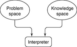
8. General structure of a heuristic search system.
Transitions from one state to another are effected by appealing to the contents of the agent’s knowledge space (the contents of a long-term memory). Elements from this knowledge space are selected and applied to a ‘current state’ in the problem space resulting in a new state. The organ that does this is shown in Figure 8 as the interpreter (on which more later). The successive applications of knowledge elements in effect result in the agent conducting a search for a solution through the problem space. This search process constitutes a computation. The problem is solved when, beginning with the initial state, the application of a sequence of knowledge elements results in the goal state being reached.
However, since a problem space may be arbitrarily large, the search through it is not randomly conducted. Rather, the agent deploys heuristics to control the amount of search, to prune away parts of the search space as unnecessary, and thereby converge to a solution as rapidly as possible.
Weak methods and strong methods
The heart of the heuristic search paradigm is, thus, the heuristics contained in the knowledge space. These may range from the very general—applicable to a wide range of problem domains—to the very specific—relevant to particular problem domains. The former are called weak methodsand the latter strong methods. In general, when the problem domain is poorly understood weak methods are more promising; when the problem domain is known or understood in more detail strong methods are more appropriate.
One effective weak method (which we have encountered several times already) is divide-and-rule. Another is called means-ends analysis:
Given a current problem state and a goal state, determine the difference between the two. Then reduce the difference by applying a relevant ‘operator’. If, however, the necessary precondition for the operator to apply is not satisfied, reduce the difference between the current state and the precondition by recursively applying means-ends analysis to the pair, current state and precondition.
An example of a problem to which both divide-and-conquer and means-ends analysis can apply together is that of a student planning her degree program. Divide-and-conquer decomposes the problem into subproblems corresponding to each of the years of the degree program. The original goal state (to graduate in a particular subject in X number of years, say) is decomposed into ‘subgoal’ states for each of the X years. For each year, the student will identify the initial state for that year (the courses already taken before that year) and attempt to identify courses to be taken that eliminate the difference between the initial and goal states for that year. The search for courses is narrowed by selecting those that are mandatory. But some of these courses may require prerequisites. Thus means-ends analysis is applied to reduce the gap between the initial state and the prerequisites. And so on.
Notice that means-ends analysis is a recursive strategy (see Chapter 3). So what is so ‘heuristic’ about it? The point is that there is no guarantee that in a particular problem domain, means-ends analysis will terminate successfully. For example, given a current state and a goal state, several actions may be applicable to reduce the difference. The action chosen may determine the difference between success and failure.
Strong methods usually represent expert knowledge of the kind specialists in a problem domain possess through formal education, hands-on training, and experience. Computational systems that determine the molecular structure of chemicals or aid engineers in their design projects are typical instances. These heuristics are often represented in the knowledge space as rules (called productions) of the form:
IF condition THEN action.
That is, if the current state in the problem space matches the ‘condition’ part of a production then the corresponding ‘action’ may be taken. As an example from the domain of digital circuit design (and implemented as part of a heuristic design automation system):
IF the goal of the circuit module is to convert a serial signal to a parallel one
THEN use a shift register.
It is possible that the current state in the problem space is such that it matches the condition parts of several productions:
IF condition1 THEN action1;
IF condition2 THEN action2.
…………..
IF conditionM THEN actionM.
In such a situation the choice of an action to take may have to be guided by a higher level heuristic (e.g. select the first matching production). This may turn out to be a wrong choice as realized later in the computation, in which case the system must ‘backtrack’ to a prior state and explore some other production.
Interpreting heuristic rules
Notice the ‘interpreter’ in Figure 8. Its task is to execute a cyclic algorithm analogous to the ICycle in a physical computer (Chapter 5):
Match: Identify all the productions in the knowledge space the condition parts of which match the current state in the problem space. Collect these rules into a conflict set.
Select a preferred rule from the conflict set according to a selection heuristic.
Execute the action part of the preferred rule.
Goto Match.
Apart from the uncertainty associated with the heuristic search paradigm, the other noticeable difference from algorithms (exact or heuristic) is (as mentioned before) that in the latter all the knowledge required to execute an algorithm is embedded in the algorithm itself. In contrast, in the heuristic search paradigm almost all the knowledge is located in the knowledge space (or long-term memory). The complexity of the heuristic search paradigm lies mostly in the richness of the knowledge space.