Practical Data Science with R (2014)

Part 1. Introduction to data science

In part 1, we concentrate on the most essential tasks in data science: working with your partners, defining your problem, and examining your data.

Chapter 1 covers the lifecycle of a typical data science project. We look at the different roles and responsibilities of project team members, the different stages of a typical project, and how to define goals and set project expectations. This chapter serves as an overview of the material that we cover in the rest of the book and is organized in the same order as the topics that we present.

Chapter 2 dives into the details of loading data into R from various external formats and transforming the data into a format suitable for analysis. It also discusses the most important R data structure for a data scientist: the data frame. More details about the R programming language are covered in appendix A.

Chapters 3 and 4 cover the data exploration and treatment that you should do before proceeding to the modeling stage. In chapter 3, we discuss some of the typical problems and issues that you’ll encounter with your data and how to use summary statistics and visualization to detect those issues. In chapter 4, we discuss data treatments that will help you deal with the problems and issues in your data. We also recommend some habits and procedures that will help you better manage the data throughout the different stages of the project.

On completing part 1, you’ll understand how to define a data science project, and you’ll know how to load data into R and prepare it for modeling and analysis.

Chapter 1. The data science process

This chapter covers

· Defining data science project roles

· Understanding the stages of a data science project

· Setting expectations for a new data science project

The data scientist is responsible for guiding a data science project from start to finish. Success in a data science project comes not from access to any one exotic tool, but from having quantifiable goals, good methodology, cross-discipline interactions, and a repeatable workflow.

This chapter walks you through what a typical data science project looks like: the kinds of problems you encounter, the types of goals you should have, the tasks that you’re likely to handle, and what sort of results are expected.

1.1. The roles in a data science project

Data science is not performed in a vacuum. It’s a collaborative effort that draws on a number of roles, skills, and tools. Before we talk about the process itself, let’s look at the roles that must be filled in a successful project. Project management has been a central concern of software engineering for a long time, so we can look there for guidance. In defining the roles here, we’ve borrowed some ideas from Fredrick Brooks’s The Mythical Man-Month: Essays on Software Engineering (Addison-Wesley, 1995) “surgical team” perspective on software development and also from the agile software development paradigm.

1.1.1. Project roles

Let’s look at a few recurring roles in a data science project in table 1.1.

Table 1.1. Data science project roles and responsibilities

Sometimes these roles may overlap. Some roles—in particular client, data architect, and operations—are often filled by people who aren’t on the data science project team, but are key collaborators.

Project sponsor

The most important role in a data science project is the project sponsor. The sponsor is the person who wants the data science result; generally they represent the business interests. The sponsor is responsible for deciding whether the project is a success or failure. The data scientist may fill the sponsor role for their own project if they feel they know and can represent the business needs, but that’s not the optimal arrangement. The ideal sponsor meets the following condition: if they’re satisfied with the project outcome, then the project is by definition a success. Getting sponsor sign-off becomes the central organizing goal of a data science project.

Keep the sponsor informed and involved

It’s critical to keep the sponsor informed and involved. Show them plans, progress, and intermediate successes or failures in terms they can understand. A good way to guarantee project failure is to keep the sponsor in the dark.

To ensure sponsor sign-off, you must get clear goals from them through directed interviews. You attempt to capture the sponsor’s expressed goals as quantitative statements. An example goal might be “Identify 90% of accounts that will go into default at least two months before the first missed payment with a false positive rate of no more than 25%.” This is a precise goal that allows you to check in parallel if meeting the goal is actually going to make business sense and whether you have data and tools of sufficient quality to achieve the goal.

Client

While the sponsor is the role that represents the business interest, the client is the role that represents the model’s end users’ interests. Sometimes the sponsor and client roles may be filled by the same person. Again, the data scientist may fill the client role if they can weight business trade-offs, but this isn’t ideal.

The client is more hands-on than the sponsor; they’re the interface between the technical details of building a good model and the day-to-day work process into which the model will be deployed. They aren’t necessarily mathematically or statistically sophisticated, but are familiar with the relevant business processes and serve as the domain expert on the team. In the loan application example that we discuss later in this chapter, the client may be a loan officer or someone who represents the interests of loan officers.

As with the sponsor, you should keep the client informed and involved. Ideally you’d like to have regular meetings with them to keep your efforts aligned with the needs of the end users. Generally the client belongs to a different group in the organization and has other responsibilities beyond your project. Keep meetings focused, present results and progress in terms they can understand, and take their critiques to heart. If the end users can’t or won’t use your model, then the project isn’t a success, in the long run.

Data scientist

The next role in a data science project is the data scientist, who’s responsible for taking all necessary steps to make the project succeed, including setting the project strategy and keeping the client informed. They design the project steps, pick the data sources, and pick the tools to be used. Since they pick the techniques that will be tried, they have to be well informed about statistics and machine learning. They’re also responsible for project planning and tracking, though they may do this with a project management partner.

At a more technical level, the data scientist also looks at the data, performs statistical tests and procedures, applies machine learning models, and evaluates results—the science portion of data science.

Data architect

The data architect is responsible for all of the data and its storage. Often this role is filled by someone outside of the data science group, such as a database administrator or architect. Data architects often manage data warehouses for many different projects, and they may only be available for quick consultation.

Operations

The operations role is critical both in acquiring data and delivering the final results. The person filling this role usually has operational responsibilities outside of the data science group. For example, if you’re deploying a data science result that affects how products are sorted on an online shopping site, then the person responsible for running the site will have a lot to say about how such a thing can be deployed. This person will likely have constraints on response time, programming language, or data size that you need to respect in deployment. The person in the operations role may already be supporting your sponsor or your client, so they’re often easy to find (though their time may be already very much in demand).

1.2. Stages of a data science project

The ideal data science environment is one that encourages feedback and iteration between the data scientist and all other stakeholders. This is reflected in the lifecycle of a data science project. Even though this book, like any other discussions of the data science process, breaks up the cycle into distinct stages, in reality the boundaries between the stages are fluid, and the activities of one stage will often overlap those of other stages. Often, you’ll loop back and forth between two or more stages before moving forward in the overall process. This is shown in figure 1.1.

Figure 1.1. The lifecycle of a data science project: loops within loops

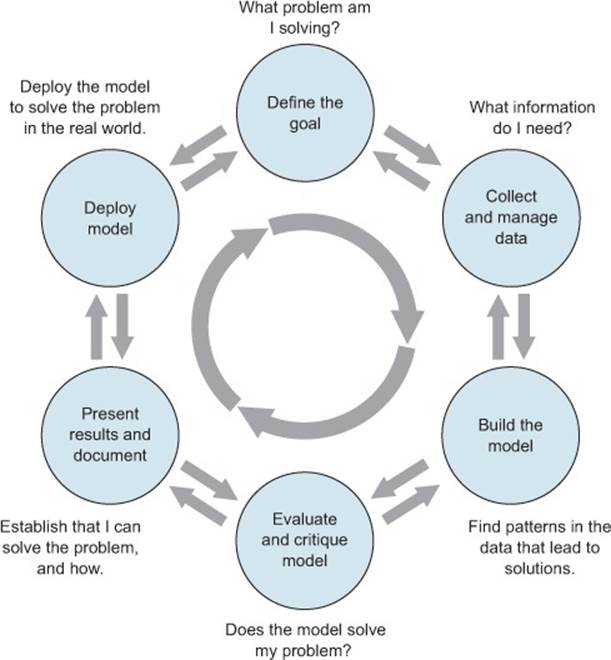
Even after you complete a project and deploy a model, new issues and questions can arise from seeing that model in action. The end of one project may lead into a follow-up project.

Let’s look at the different stages shown in figure 1.1. As a real-world example, suppose you’re working for a German bank.^[1] The bank feels that it’s losing too much money to bad loans and wants to reduce its losses. This is where your data science team comes in.

¹ For this chapter, we use a credit dataset donated by Professor Dr. Hans Hofmann to the UCI Machine Learning Repository in 1994. We’ve simplified some of the column names for clarity. The dataset can be found at http://archive.ics.uci.edu/ml/datasets/Statlog+(German+Credit+Data). We show how to load this data and prepare it for analysis in chapter 2. Note that the German currency at the time of data collection was the deutsch mark (DM).

1.2.1. Defining the goal

The first task in a data science project is to define a measurable and quantifiable goal. At this stage, learn all that you can about the context of your project:

· Why do the sponsors want the project in the first place? What do they lack, and what do they need?

· What are they doing to solve the problem now, and why isn’t that good enough?

· What resources will you need: what kind of data and how much staff? Will you have domain experts to collaborate with, and what are the computational resources?

· How do the project sponsors plan to deploy your results? What are the constraints that have to be met for successful deployment?

Let’s come back to our loan application example. The ultimate business goal is to reduce the bank’s losses due to bad loans. Your project sponsor envisions a tool to help loan officers more accurately score loan applicants, and so reduce the number of bad loans made. At the same time, it’s important that the loan officers feel that they have final discretion on loan approvals.

Once you and the project sponsor and other stakeholders have established preliminary answers to these questions, you and they can start defining the precise goal of the project. The goal should be specific and measurable, not “We want to get better at finding bad loans,” but instead, “We want to reduce our rate of loan charge-offs by at least 10%, using a model that predicts which loan applicants are likely to default.”

A concrete goal begets concrete stopping conditions and concrete acceptance criteria. The less specific the goal, the likelier that the project will go unbounded, because no result will be “good enough.” If you don’t know what you want to achieve, you don’t know when to stop trying—or even what to try. When the project eventually terminates—because either time or resources run out—no one will be happy with the outcome.

This doesn’t mean that more exploratory projects aren’t needed at times: “Is there something in the data that correlates to higher defaults?” or “Should we think about reducing the kinds of loans we give out? Which types might we eliminate?” In this situation, you can still scope the project with concrete stopping conditions, such as a time limit. The goal is then to come up with candidate hypotheses. These hypotheses can then be turned into concrete questions or goals for a full-scale modeling project.

Once you have a good idea of the project’s goals, you can focus on collecting data to meet those goals.

1.2.2. Data collection and management

This step encompasses identifying the data you need, exploring it, and conditioning it to be suitable for analysis. This stage is often the most time-consuming step in the process. It’s also one of the most important:

· What data is available to me?

· Will it help me solve the problem?

· Is it enough?

· Is the data quality good enough?

Imagine that for your loan application problem, you’ve collected a sample of representative loans from the last decade (excluding home loans). Some of the loans have defaulted; most of them (about 70%) have not. You’ve collected a variety of attributes about each loan application, as listed in table 1.2.

Table 1.2. Loan data attributes

In your data, Good.Loan takes on two possible values: GoodLoan and BadLoan. For the purposes of this discussion, assume that a GoodLoan was paid off, and a BadLoan defaulted.

As much as possible, try to use information that can be directly measured, rather than information that is inferred from another measurement. For example, you might be tempted to use income as a variable, reasoning that a lower income implies more difficulty paying off a loan. The ability to pay off a loan is more directly measured by considering the size of the loan payments relative to the borrower’s disposable income. This information is more useful than income alone; you have it in your data as the variableInstallment.rate.in.percentage.of.disposable.income.

This is the stage where you conduct initial exploration and visualization of the data. You’ll also clean the data: repair data errors and transform variables, as needed. In the process of exploring and cleaning the data, you may discover that it isn’t suitable for your problem, or that you need other types of information as well. You may discover things in the data that raise issues more important than the one you originally planned to address. For example, the data in figure 1.2 seems counterintuitive.

Figure 1.2. The fraction of defaulting loans by credit history category. The dark region of each bar represents the fraction of loans in that category that defaulted.

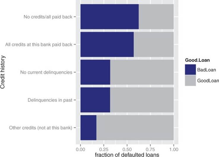
Why would some of the seemingly safe applicants (those who repaid all credits to the bank) default at a higher rate than seemingly riskier ones (those who had been delinquent in the past)? After looking more carefully at the data and sharing puzzling findings with other stakeholders and domain experts, you realize that this sample is inherently biased: you only have loans that were actually made (and therefore already accepted). Overall, there are fewer risky-looking loans than safe-looking ones in the data. The probable story is that risky-looking loans were approved after a much stricter vetting process, a process that perhaps the safe-looking loan applications could bypass. This suggests that if your model is to be used downstream of the current application approval process, credit history is no longer a useful variable. It also suggests that even seemingly safe loan applications should be more carefully scrutinized.

Discoveries like this may lead you and other stakeholders to change or refine the project goals. In this case, you may decide to concentrate on the seemingly safe loan applications. It’s common to cycle back and forth between this stage and the previous one, as well as between this stage and the modeling stage, as you discover things in the data. We’ll cover data exploration and management in depth in chapters 3 and 4.

1.2.3. Modeling

You finally get to statistics and machine learning during the modeling, or analysis, stage. Here is where you try to extract useful insights from the data in order to achieve your goals. Since many modeling procedures make specific assumptions about data distribution and relationships, there will be overlap and back-and-forth between the modeling stage and the data cleaning stage as you try to find the best way to represent the data and the best form in which to model it.

The most common data science modeling tasks are these:

· Classification— Deciding if something belongs to one category or another

· Scoring— Predicting or estimating a numeric value, such as a price or probability

· Ranking— Learning to order items by preferences

· Clustering— Grouping items into most-similar groups

· Finding relations— Finding correlations or potential causes of effects seen in the data

· Characterization— Very general plotting and report generation from data

For each of these tasks, there are several different possible approaches. We’ll cover some of the most common approaches to the different tasks in this book.

The loan application problem is a classification problem: you want to identify loan applicants who are likely to default. Three common approaches in such cases are logistic regression, Naive Bayes classifiers, and decision trees (we’ll cover these methods in-depth in future chapters). You’ve been in conversation with loan officers and others who would be using your model in the field, so you know that they want to be able to understand the chain of reasoning behind the model’s classification, and they want an indication of how confident the model is in its decision: is this applicant highly likely to default, or only somewhat likely? Given the preceding desiderata, you decide that a decision tree is most suitable. We’ll cover decision trees more extensively in a future chapter, but for now the call in R is as shown in the following listing (you can download data from https://github.com/WinVector/zmPDSwR/tree/master/Statlog).^[2]

² In this chapter, for clarity of illustration we deliberately fit a small and shallow tree.

Listing 1.1. Building a decision tree

library('rpart')

load('GCDData.RData')

model <- rpart(Good.Loan ~

Duration.in.month +

Installment.rate.in.percentage.of.disposable.income +

Credit.amount +

Other.installment.plans,

data=d,

control=rpart.control(maxdepth=4),

method="class")

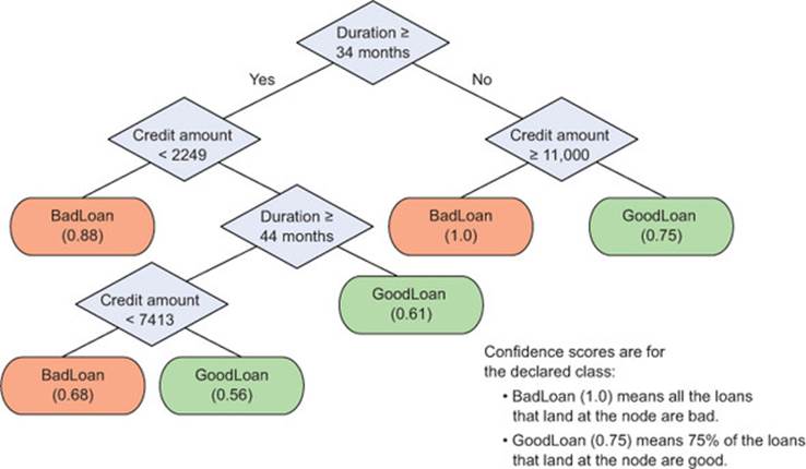
Let’s suppose that you discover the model shown in figure 1.3.

Figure 1.3. A decision tree model for finding bad loan applications, with confidence scores

We’ll discuss general modeling strategies in chapter 5 and go into details of specific modeling algorithms in part 2.

1.2.4. Model evaluation and critique

Once you have a model, you need to determine if it meets your goals:

· Is it accurate enough for your needs? Does it generalize well?

· Does it perform better than “the obvious guess”? Better than whatever estimate you currently use?

· Do the results of the model (coefficients, clusters, rules) make sense in the context of the problem domain?

If you’ve answered “no” to any of these questions, it’s time to loop back to the modeling step—or decide that the data doesn’t support the goal you’re trying to achieve. No one likes negative results, but understanding when you can’t meet your success criteria with current resources will save you fruitless effort. Your energy will be better spent on crafting success. This might mean defining more realistic goals or gathering the additional data or other resources that you need to achieve your original goals.

Returning to the loan application example, the first thing to check is that the rules that the model discovered make sense. Looking at figure 1.3, you don’t notice any obviously strange rules, so you can go ahead and evaluate the model’s accuracy. A good summary of classifier accuracy is theconfusion matrix, which tabulates actual classifications against predicted ones.^[3]

³ Normally, we’d evaluate the model against a test set (data that wasn’t used to build the model). In this example, for simplicity, we evaluate the model against the training data (data that was used to build the model).

Listing 1.2. Plotting the confusion matrix

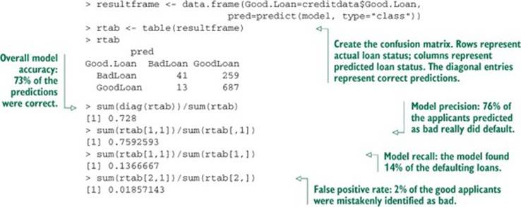
The model predicted loan status correctly 73% of the time—better than chance (50%). In the original dataset, 30% of the loans were bad, so guessing GoodLoan all the time would be 70% accurate (though not very useful). So you know that the model does better than random and somewhat better than obvious guessing.

Overall accuracy is not enough. You want to know what kinds of mistakes are being made. Is the model missing too many bad loans, or is it marking too many good loans as bad? Recall measures how many of the bad loans the model can actually find. Precision measures how many of the loans identified as bad really are bad. False positive rate measures how many of the good loans are mistakenly identified as bad. Ideally, you want the recall and the precision to be high, and the false positive rate to be low. What constitutes “high enough” and “low enough” is a decision that you make together with the other stakeholders. Often, the right balance requires some trade-off between recall and precision.

There are other measures of accuracy and other measures of the quality of a model, as well. We’ll talk about model evaluation in chapter 5.

1.2.5. Presentation and documentation

Once you have a model that meets your success criteria, you’ll present your results to your project sponsor and other stakeholders. You must also document the model for those in the organization who are responsible for using, running, and maintaining the model once it has been deployed.

Different audiences require different kinds of information. Business-oriented audiences want to understand the impact of your findings in terms of business metrics. In our loan example, the most important thing to present to business audiences is how your loan application model will reduce charge-offs (the money that the bank loses to bad loans). Suppose your model identified a set of bad loans that amounted to 22% of the total money lost to defaults. Then your presentation or executive summary should emphasize that the model can potentially reduce the bank’s losses by that amount, as shown in figure 1.4.

Figure 1.4. Notional slide from an executive presentation

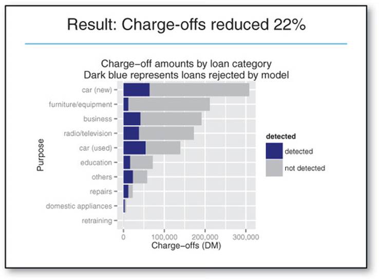
You also want to give this audience your most interesting findings or recommendations, such as that new car loans are much riskier than used car loans, or that most losses are tied to bad car loans and bad equipment loans (assuming that the audience didn’t already know these facts). Technical details of the model won’t be as interesting to this audience, and you should skip them or only present them at a high level.

A presentation for the model’s end users (the loan officers) would instead emphasize how the model will help them do their job better:

· How should they interpret the model?

· What does the model output look like?

· If the model provides a trace of which rules in the decision tree executed, how do they read that?

· If the model provides a confidence score in addition to a classification, how should they use the confidence score?

· When might they potentially overrule the model?

Presentations or documentation for operations staff should emphasize the impact of your model on the resources that they’re responsible for.

We’ll talk about the structure of presentations and documentation for various audiences in part 3.

1.2.6. Model deployment and maintenance

Finally, the model is put into operation. In many organizations this means the data scientist no longer has primary responsibility for the day-to-day operation of the model. But you still should ensure that the model will run smoothly and won’t make disastrous unsupervised decisions. You also want to make sure that the model can be updated as its environment changes. And in many situations, the model will initially be deployed in a small pilot program. The test might bring out issues that you didn’t anticipate, and you may have to adjust the model accordingly. We’ll discuss model deployment considerations in chapter 10.

For example, you may find that loan officers frequently override the model in certain situations because it contradicts their intuition. Is their intuition wrong? Or is your model incomplete? Or, in a more positive scenario, your model may perform so successfully that the bank wants you to extend it to home loans as well.

Before we dive deeper into the stages of the data science lifecycle in the following chapters, let’s look at an important aspect of the initial project design stage: setting expectations.

1.3. Setting expectations

Setting expectations is a crucial part of defining the project goals and success criteria. The business-facing members of your team (in particular, the project sponsor) probably already have an idea of the performance required to meet business goals: for example, the bank wants to reduce their losses from bad loans by at least 10%. Before you get too deep into a project, you should make sure that the resources you have are enough for you to meet the business goals.

In this section, we discuss ways to estimate whether the data you have available is good enough to potentially meet desired accuracy goals. This is an example of the fluidity of the project lifecycle stages. You get to know the data better during the exploration and cleaning phase; after you have a sense of the data, you can get a sense of whether the data is good enough to meet desired performance thresholds. If it’s not, then you’ll have to revisit the project design and goal-setting stage.

1.3.1. Determining lower and upper bounds on model performance

Understanding how well a model should do for acceptable performance and how well it can do given the available data are both important when defining acceptance criteria.

The null model: a lower bound on performance

You can think of the null model as being “the obvious guess” that your model must do better than. In situations where there’s a working model or solution already in place that you’re trying to improve, the null model is the existing solution. In situations where there’s no existing model or solution, the null model is the simplest possible model (for example, always guessing GoodLoan, or always predicting the mean value of the output, when you’re trying to predict a numerical value). The null model represents the lower bound on model performance that you should strive for.

In our loan application example, 70% of the loan applications in the dataset turned out to be good loans. A model that labels all loans as GoodLoan (in effect, using only the existing process to classify loans) would be correct 70% of the time. So you know that any actual model that you fit to the data should be better than 70% accurate to be useful. Since this is the simplest possible model, its error rate is called the base error rate.

How much better than 70% should you be? In statistics there’s a procedure called hypothesis testing, or significance testing, that tests whether your model is equivalent to a null model (in this case, whether a new model is basically only as accurate as guessing GoodLoan all the time). You want your model’s accuracy to be “significantly better”—in statistical terms—than 70%. We’ll cover the details of significance testing in chapter 5.

Accuracy is not the only (or even the best) performance metric. In our example, the null model would have zero recall in identifying bad loans, which obviously is not what you want. Generally if there is an existing model or process in place, you’d like to have an idea of its precision, recall, and false positive rates; if the purpose of your project is to improve the existing process, then the current model must be unsatisfactory for at least one of these metrics. This also helps you determine lower bounds on desired performance.

The Bayes rate: an upper bound on model performance

The business-dictated performance goals will of course be higher than the lower bounds discussed here. You should try to make sure as early as possible that you have the data to meet your goals.

One thing to look at is what statisticians call the unexplainable variance: how much of the variation in your output can’t be explained by your input variables. Let’s take a very simple example: suppose you want to use the rule of thumb that loans that equal more than 15% of the borrower’s disposable income will default; otherwise, loans are good. You want to know if this rule alone will meet your goal of predicting bad loans with at least 85% accuracy. Let’s consider the two populations next.

Listing 1.3. Plotting the relation between disposable income and loan outcome

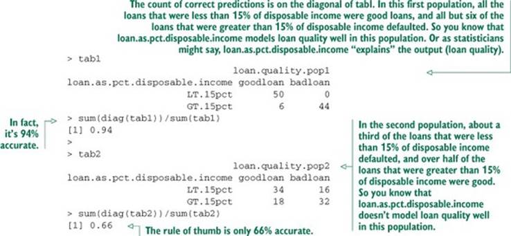
For the second population, you know that you can’t meet your goals using only loan.as.pct.disposable.income. To build a more accurate model, you’ll need additional input variables.

The limit on prediction accuracy due to unexplainable variance is known as the Bayes rate. You can think of the Bayes rate as describing the best accuracy you can achieve given your data. If the Bayes rate doesn’t meet your business-dictated performance goals, then you shouldn’t start the project without revisiting your goals or finding additional data to improve your model.^[4]

⁴ The Bayes rate gives the best possible accuracy, but the most accurate model doesn’t always have the best possible precision or recall (though it may represent the best trade-off of the two).

Exactly finding the Bayes rate is not always possible—if you could always find the best possible model, then your job would already be done. If all your variables are discrete (and you have a lot of data), you can find the Bayes rate by building a lookup table for all possible variable combinations. In other situations, a nearest-neighbor classifier (we’ll discuss them in chapter 8) can give you a good estimate of the Bayes rate, even though a nearest-neighbor classifier may not be practical to deploy as an actual production model. In any case, you should try to get some idea of the limitations of your data early in the process, so you know whether it’s adequate to meet your goals.

1.4. Summary

The data science process involves a lot of back-and-forth—between the data scientist and other project stakeholders, and between the different stages of the process. Along the way, you’ll encounter surprises and stumbling blocks; this book will teach you procedures for overcoming some of these hurdles. It’s important to keep all the stakeholders informed and involved; when the project ends, no one connected with it should be surprised by the final results.

In the next chapters, we’ll look at the stages that follow project design: loading, exploring, and managing the data. Chapter 2 covers a few basic ways to load the data into R, in a format that’s convenient for analysis.

Key takeaways

· A successful data science project involves more than just statistics. It also requires a variety of roles to represent business and client interests, as well as operational concerns.

· Make sure you have a clear, verifiable, quantifiable goal.

· Make sure you’ve set realistic expectations for all stakeholders.