Practical Data Science with R (2014)
Part 1. Introduction to data science
Chapter 2. Loading data into R
This chapter covers
· Understanding R’s data frame structure
· Loading data into R from files and from relational databases
· Transforming data for analysis
If your experience has been like ours, many of your data science projects start when someone points you toward a bunch of data and you’re left to make sense of it. Your first thought may be to use shell tools or spreadsheets to sort through it, but you quickly realize that you’re taking more time tinkering with the tools than actually analyzing the data. Luckily, there’s a better way. In this chapter, we’ll demonstrate how to quickly load and start working with data using R. Using R to transform data is easy because R’s main data type (the data frame) is ideal for working with structured data, and R has adapters that read data from many common data formats. In this chapter, we’ll start with small example datasets found in files and then move to datasets from relational databases. By the end of the chapter, you’ll be able to confidently use R to extract, transform, and load data for analysis.[1]
1 We’ll demonstrate and comment on the R commands necessary to prepare the data, but if you’re unfamiliar with programming in R, we recommend at least skimming appendix A or consulting a good book on R such as R in Action, Second Edition (Robert Kabacoff, Manning Publications (2014), http://mng.bz/ybS4). All the tools you need are freely available and we provide instructions how to download and start working with them in appendix A.
For our first example, let’s start with some example datasets from files.
2.1. Working with data from files
The most common ready-to-go data format is a family of tabular formats called structured values. Most of the data you find will be in (or nearly in) one of these formats. When you can read such files into R, you can analyze data from an incredible range of public and private data sources. In this section, we’ll work on two examples of loading data from structured files, and one example of loading data directly from a relational database. The point is to get data quickly into R so we can then use R to perform interesting analyses.
2.1.1. Working with well-structured data from files or URLs
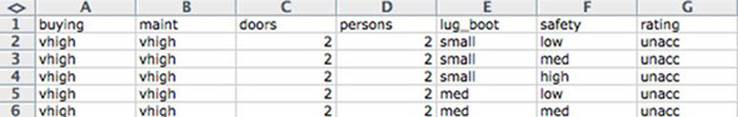
The easiest data format to read is table-structured data with headers. As shown in figure 2.1, this data is arranged in rows and columns where the first row gives the column names. Each column represents a different fact or measurement; each row represents an instance or datum about which we know the set of facts. A lot of public data is in this format, so being able to read it opens up a lot of opportunities.
Figure 2.1. Car data viewed as a table
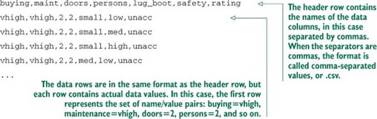
Before we load the German credit data that we used in the previous chapter, let’s demonstrate the basic loading commands with a simple data file from the University of California Irvine Machine Learning Repository (http://archive.ics.uci.edu/ml/). The UCI data files tend to come without headers, so to save steps (and to keep it very basic, at this point) we’ve pre-prepared our first data example from the UCI car dataset: http://archive.ics.uci.edu/ml/machine-learning-databases/car/. Our pre-prepared file is at http://win-vector.com/dfiles/car.data.csv and looks like the following (details found at https://github.com/WinVector/zmPDSwR/tree/master/UCICar):
Avoid “by hand” steps
We strongly encourage you to avoid performing any steps “by hand” when importing data. It’s tempting to use an editor to add a header line to a file, as we did in our example. A better strategy is to write a script either outside R (using shell tools) or inside R to perform any necessary reformatting. Automating these steps greatly reduces the amount of trauma and work during the inevitable data refresh.
Notice that this file is already structured like a spreadsheet with easy-to-identify rows and columns. The data shown here is claimed to be the details about recommendations on cars, but is in fact made-up examples used to test some machine-learning theories. Each (nonheader) row represents a review of a different model of car. The columns represent facts about each car model. Most of the columns are objective measurements (purchase cost, maintenance cost, number of doors, and so on) and the final column “rating” is marked with the overall rating (vgood, good, acc, andunacc). These sorts of explanations can’t be found in the data but must be extracted from the documentation found with the original data.
Loading well-structured data from files or URLs
Loading data of this type into R is a one-liner: we use the R command read.table() and we’re done. If data were always in this format, we’d meet all of the goals of this section and be ready to move on to modeling with just the following code.
Listing 2.1. Reading the UCI car data
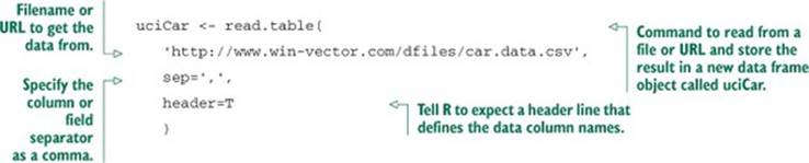
This loads the data and stores it in a new R data frame object called uciCar. Data frames are R’s primary way of representing data and are well worth learning to work with (as we discuss in our appendixes). The read.table() command is powerful and flexible; it can accept many different types of data separators (commas, tabs, spaces, pipes, and others) and it has many options for controlling quoting and escaping data. read.table() can read from local files or remote URLs. If a resource name ends with the .gz suffix, read.table() assumes the file has been compressed in gzip style and will automatically decompress it while reading.
Examining our data
Once we’ve loaded the data into R, we’ll want to examine it. The commands to always try first are these:
· class()— Tells you what type of R object you have. In our case, class(uciCar) tells us the object uciCar is of class data.frame.
· help()— Gives you the documentation for a class. In particular try help (class(uciCar)) or help("data.frame").
· summary()— Gives you a summary of almost any R object. summary(uciCar) shows us a lot about the distribution of the UCI car data.
For data frames, the command dim() is also important, as it shows you how many rows and columns are in the data. We show the results of a few of these steps next (steps are prefixed by > and R results are shown after each step).
Listing 2.2. Exploring the car data
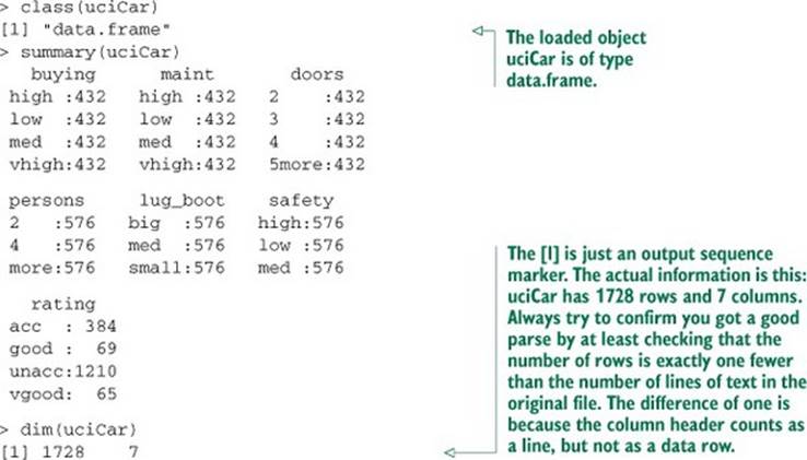
The summary() command shows us the distribution of each variable in the dataset. For example, we know each car in the dataset was declared to seat 2, 4 or more persons, and we know there were 576 two-seater cars in the dataset. Already we’ve learned a lot about our data, without having to spend a lot of time setting pivot tables as we would have to in a spreadsheet.
Working with other data formats
.csv is not the only common data file format you’ll encounter. Other formats include .tsv (tab-separated values), pipe-separated files, Microsoft Excel workbooks, JSON data, and XML. R’s built-in read.table() command can be made to read most separated value formats. Many of the deeper data formats have corresponding R packages:
· XLS/XLSX—http://cran.r-project.org/doc/manuals/R-data.html#Reading-Excel-spreadsheets
· JSON—http://cran.r-project.org/web/packages/rjson/index.html
· XML—http://cran.r-project.org/web/packages/XML/index.html
· MongoDB—http://cran.r-project.org/web/packages/rmongodb/index.html
· SQL—http://cran.r-project.org/web/packages/DBI/index.html
2.1.2. Using R on less-structured data
Data isn’t always available in a ready-to-go format. Data curators often stop just short of producing a ready-to-go machine-readable format. The German bank credit dataset discussed in chapter 1 is an example of this. This data is stored as tabular data without headers; it uses a cryptic encoding of values that requires the dataset’s accompanying documentation to untangle. This isn’t uncommon and is often due to habits or limitations of other tools that commonly work with the data. Instead of reformatting the data before we bring it into R, as we did in the last example, we’ll now show how to reformat the data using R. This is a much better practice, as we can save and reuse the R commands needed to prepare the data.
Details of the German bank credit dataset can be found at http://mng.bz/mZbu. We’ll show how to transform this data into something meaningful using R. After these steps, you can perform the analysis already demonstrated in chapter 1. As we can see in our file excerpt, the data is an incomprehensible block of codes with no meaningful explanations:
A11 6 A34 A43 1169 A65 A75 4 A93 A101 4 ...
A12 48 A32 A43 5951 A61 A73 2 A92 A101 2 ...
A14 12 A34 A46 2096 A61 A74 2 A93 A101 3 ...
...
Transforming data in R
Data often needs a bit of transformation before it makes any sense. In order to decrypt troublesome data, you need what’s called the schema documentation or a data dictionary. In this case, the included dataset description says the data is 20 input columns followed by one result column. In this example, there’s no header in the data file. The column definitions and the meaning of the cryptic A-* codes are all in the accompanying data documentation. Let’s start by loading the raw data into R. We can either save the data to a file or let R load the data directly from the URL. Start a copy of R or RStudio (see appendix A) and type in the commands in the following listing.
Listing 2.3. Loading the credit dataset
d <- read.table(paste('http://archive.ics.uci.edu/ml/',
'machine-learning-databases/statlog/german/german.data',sep=''),
stringsAsFactors=F,header=F)
print(d[1:3,])
Notice that this prints out the exact same three rows we saw in the raw file with the addition of column names V1 through V21. We can change the column names to something meaningful with the command in the following listing.
Listing 2.4. Setting column names
colnames(d) <- c('Status.of.existing.checking.account',
'Duration.in.month', 'Credit.history', 'Purpose',
'Credit.amount', 'Savings account/bonds',
'Present.employment.since',
'Installment.rate.in.percentage.of.disposable.income',
'Personal.status.and.sex', 'Other.debtors/guarantors',
'Present.residence.since', 'Property', 'Age.in.years',
'Other.installment.plans', 'Housing',
'Number.of.existing.credits.at.this.bank', 'Job',
'Number.of.people.being.liable.to.provide.maintenance.for',
'Telephone', 'foreign.worker', 'Good.Loan')
d$Good.Loan <- as.factor(ifelse(d$Good.Loan==1,'GoodLoan','BadLoan'))
print(d[1:3,])
The c() command is R’s method to construct a vector. We copied the names directly from the dataset documentation. By assigning our vector of names into the data frame’s colnames() slot, we’ve reset the data frame’s column names to something sensible. We can find what slots and commands our data frame d has available by typing help(class(d)).
The data documentation further tells us the column names, and also has a dictionary of the meanings of all of the cryptic A-* codes. For example, it says in column 4 (now called Purpose, meaning the purpose of the loan) that the code A40 is a new car loan, A41 is a used car loan, and so on. We copied 56 such codes into an R list that looks like the next listing.
Listing 2.5. Building a map to interpret loan use codes
mapping <- list(
'A40'='car (new)',
'A41'='car (used)',
'A42'='furniture/equipment',
'A43'='radio/television',
'A44'='domestic appliances',
...
)
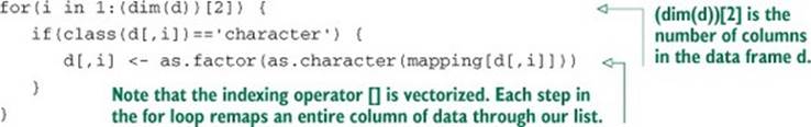
Lists are R’s map structures
Lists are R’s map structures. They can map strings to arbitrary objects. The important list operations [] and %in% are vectorized. This means that, when applied to a vector of values, they return a vector of results by performing one lookup per entry.
With the mapping list defined, we can then use the following for loop to convert values in each column that was of type character from the original cryptic A-* codes into short level descriptions taken directly from the data documentation. We, of course, skip any such transform for columns that contain numeric data.
Listing 2.6. Transforming the car data
We share the complete set of column preparations for this dataset here: https://github.com/WinVector/zmPDSwR/tree/master/Statlog/. We encourage readers to download the data and try these steps themselves.
Examining our new data
We can now easily examine the purpose of the first three loans with the command print(d[1:3,'Purpose']). We can look at the distribution of loan purpose with summary(d$Purpose) and even start to investigate the relation of loan type to loan outcome, as shown in the next listing.
Listing 2.7. Summary of Good.Loan and Purpose
> table(d$Purpose,d$Good.Loan)
BadLoan GoodLoan
business 34 63
car (new) 89 145
car (used) 17 86
domestic appliances 4 8
education 22 28
furniture/equipment 58 123
others 5 7
radio/television 62 218
repairs 8 14
retraining 1 8
You should now be able to load data from files. But a lot of data you want to work with isn’t in files; it’s in databases. So it’s important that we work through how to load data from databases directly into R.
2.2. Working with relational databases
In many production environments, the data you want lives in a relational or SQL database, not in files. Public data is often in files (as they are easier to share), but your most important client data is often in databases. Relational databases scale easily to the millions of records and supply important production features such as parallelism, consistency, transactions, logging, and audits. When you’re working with transaction data, you’re likely to find it already stored in a relational database, as relational databases excel at online transaction processing (OLTP).
Often you can export the data into a structured file and use the methods of our previous sections to then transfer the data into R. But this is generally not the right way to do things. Exporting from databases to files is often unreliable and idiosyncratic due to variations in database tools and the typically poor job these tools do when quoting and escaping characters that are confused with field separators. Data in a database is often stored in what is called a normalized form, which requires relational preparations called joins before the data is ready for analysis. Also, you often don’t want a dump of the entire database, but instead wish to freely specify which columns and aggregations you need during analysis.
The right way to work with data found in databases is to connect R directly to the database, which is what we’ll demonstrate in this section.
As a step of the demonstration, we’ll show how to load data into a database. Knowing how to load data into a database is useful for problems that need more sophisticated preparation than we’ve so far discussed. Relational databases are the right place for transformations such as joins or sampling. Let’s start working with data in a database for our next example.
2.2.1. A production-size example
For our production-size example we’ll use the United States Census 2011 national PUMS American Community Survey data found at www.census.gov/acs/www/data_documentation/pums_data/. This is a remarkable set of data involving around 3 million individuals and 1.5 million households. Each row contains over 200 facts about each individual or household (income, employment, education, number of rooms, and so on). The data has household cross-reference IDs so individuals can be joined to the household they’re in. The size of the dataset is interesting: a few gigabytes when zipped up. So it’s small enough to store on a good network or thumb drive, but larger than is convenient to work with on a laptop with R alone (which is more comfortable when working in the range of hundreds of thousands of rows).
This size—millions of rows—is the sweet spot for relational database or SQL-assisted analysis on a single machine. We’re not yet forced to move into a MapReduce or database cluster to do our work, but we do want to use a database for some of the initial data handling. We’ll work through all of the steps for acquiring this data and preparing it for analysis in R.
Curating the data
A hard rule of data science is that you must be able to reproduce your results. At the very least, be able to repeat your own successful work through your recorded steps and without depending on a stash of intermediate results. Everything must either have directions on how to produce it or clear documentation on where it came from. We call this the “no alien artifacts” discipline. For example, when we said we’re using PUMS American Community Survey data, this statement isn’t precise enough for anybody to know what data we specifically mean. Our actual notebook entry (which we keep online, so we can search it) on the PUMS data is as shown in the next listing.
Listing 2.8. PUMS data provenance documentation
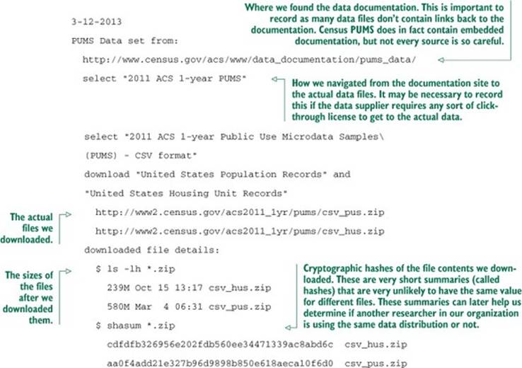
Keep notes
A big part of being a data scientist is being able to defend your results and repeat your work. We strongly advise keeping a notebook. We also strongly advise keeping all of your scripts and code under version control, as we discuss in appendix A. You absolutely need to be able to answer exactly what code and which data were used to build the results you presented last week.
Staging the data into a database
Structured data at a scale of millions of rows is best handled in a database. You can try to work with text-processing tools, but a database is much better at representing the fact that your data is arranged in both rows and columns (not just lines of text).
We’ll use three database tools in this example: the serverless database engine H2, the database loading tool SQL Screwdriver, and the database browser SQuirreL SQL. All of these are Java-based, run on many platforms, and are open source. We describe how to download and start working with all of them in appendix A.[2]
2 Other easy ways to use SQL in R include the sqldf and RSQLite packages.
If you have a database such as MySQL or PostgreSQL already available, we recommend using one of them instead of using H2.[3] To use your own database, you’ll need to know enough of your database driver and connection information to build a JDBC connection. If using H2, you’ll only need to download the H2 driver as described in appendix A, pick a file path to store your results, and pick a username and password (both are set on first use, so there are no administrative steps). H2 is a serverless zero-install relational database that supports queries in SQL. It’s powerful enough to work on PUMS data and easy to use. We show how to get H2 running in appendix A.
3 If you have access to a parallelized SQL database such as Greenplum, we strongly suggest using it to perform aggregation and preparation steps on your big data. Being able to write standard SQL queries and have them finish quickly at big data scale can be game-changing.
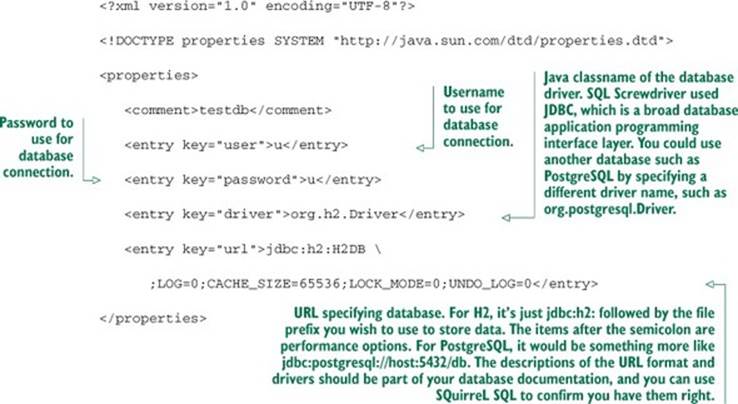
We’ll use the Java-based tool SQL Screwdriver to load the PUMS data into our database. We first copy our database credentials into a Java properties XML file.
Listing 2.9. SQL Screwdriver XML configuration file
We’ll then use Java at the command line to load the data. To load the four files containing the two tables, run the commands in the following listing.
Listing 2.10. Loading data with SQL Screwdriver
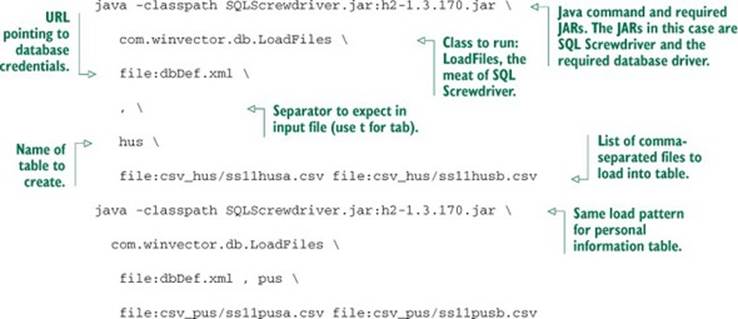
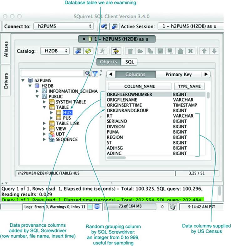
SQL Screwdriver infers data types by scanning the file and creates new tables in your database. It then populates these tables with the data. SQL Screwdriver also adds four additional “provenance” columns when loading your data. These columns are ORIGINSERTTIME, ORIGFILENAME, ORIGFILEROWNUMBER, and ORIGRANDGROUP. The first three fields record when you ran the data load, what filename the row came from, and what line the row came from. The ORIGRANDGROUP is a pseudo-random integer distributed uniformly from 0 through 999, designed to make repeatable sampling plans easy to implement. You should get in the habit of having annotations and keeping notes at each step of the process.
We can now use a database browser like SQuirreL SQL to examine this data. We start up SQuirreL SQL and copy the connection details from our XML file into a database alias, as shown in appendix A. We’re then ready to type SQL commands into the execution window. A couple of commands you can try are SELECT COUNT(1) FROM hus and SELECT COUNT(1) FROM pus, which will tell you that the hus table has 1,485,292 rows and the pus table has 3,112,017 rows. Each of the tables has over 200 columns, and there are over a billion cells of data in these two tables. We can actually do a lot more. In addition to the SQL execution panel, SQuirreL SQL has an Objects panel that allows graphical exploration of database table definitions. Figure 2.2 shows some of the columns in the hus table.
Figure 2.2. SQuirreL SQL table explorer
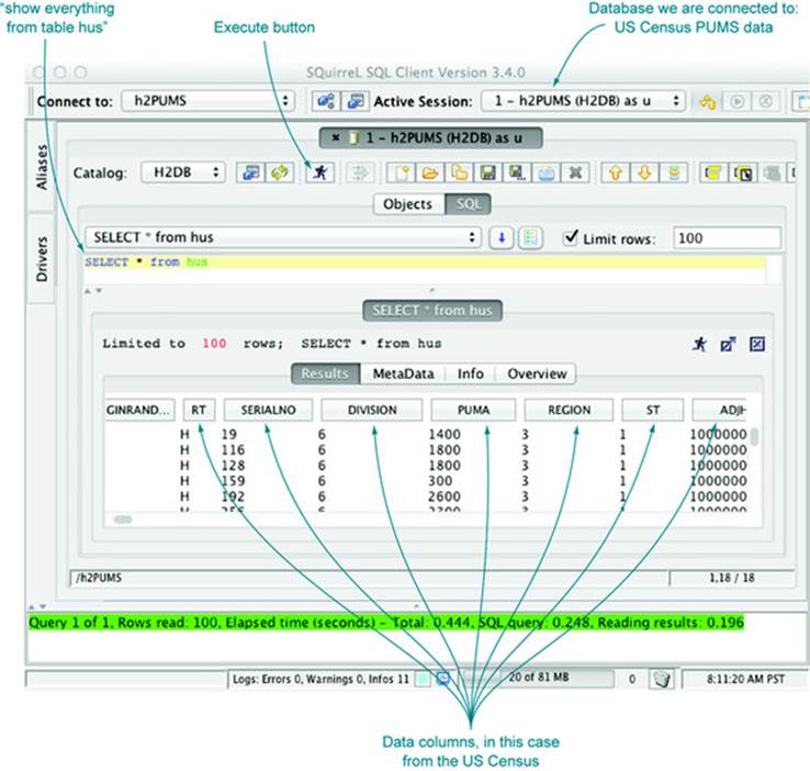
Now we can view our data as a table (as we would in a spreadsheet). We can now examine, aggregate, and summarize our data using the SQuirreL SQL database browser. Figure 2.3 shows a few example rows and columns from the household data table.
Figure 2.3. Browsing PUMS data using SQuirreL SQL
2.2.2. Loading data from a database into R
To load data from a database, we use a database connector. Then we can directly issue SQL queries from R. SQL is the most common database query language and allows us to specify arbitrary joins and aggregations. SQL is called a declarative language (as opposed to a procedurallanguage) because in SQL we specify what relations we would like our data sample to have, not how to compute them. For our example, we load a sample of the household data from the hus table and the rows from the person table (pus) that are associated with those households.[4]
4 Producing composite records that represent matches between one or more tables (in our case hus and pus) is usually done with what is called a join. For this example, we use an even more efficient pattern called a sub-select that uses the keyword in.
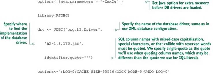
Listing 2.11. Loading data into R from a relational database
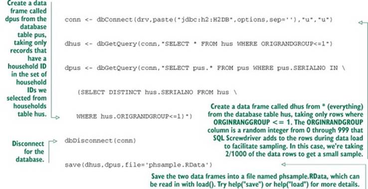
And we’re in business; the data has been unpacked from the Census-supplied .csv files into our database and a useful sample has been loaded into R for analysis. We have actually accomplished a lot. Generating, as we have, a uniform sample of households and matching people would be tedious using shell tools. It’s exactly what SQL databases are designed to do well.
Don’t be too proud to sample
Many data scientists spend too much time adapting algorithms to work directly with big data. Often this is wasted effort, as for many model types you would get almost exactly the same results on a reasonably sized data sample. You only need to work with “all of your data” when what you’re modeling isn’t well served by sampling, such as when characterizing rare events or performing bulk calculations over social networks.
Note that this data is still in some sense large (out of the range where using spreadsheets is actually reasonable). Using dim(dhus) and dim(dpus), we see that our household sample has 2,982 rows and 210 columns, and the people sample has 6,279 rows and 288 columns. All of these columns are defined in the Census documentation.
2.2.3. Working with the PUMS data
Remember that the whole point of loading data (even from a database) into R is to facilitate modeling and analysis. Data analysts should always have their “hands in the data” and always take a quick look at their data after loading it. If you’re not willing to work with the data, you shouldn’t bother loading it into R. To emphasize analysis, we’ll demonstrate how to perform a quick examination of the PUMS data.
Loading and conditioning the PUMS data
Each row of PUMS data represents a single anonymized person or household. Personal data recorded includes occupation, level of education, personal income, and many other demographics variables. To load our prepared data frame, download phsample.Rdata fromhttps://github.com/WinVector/zmPDSwR/tree/master/PUMS and run the following command in R: load('phsample.RData').
Our example problem will be to predict income (represented in US dollars in the field PINCP) using the following variables:
· Age— An integer found in column AGEP.
· Employment class— Examples: for-profit company, nonprofit company, ... found in column COW.
· Education level— Examples: no high school diploma, high school, college, and so on, found in column SCHL.
· Sex of worker— Found in column SEX.
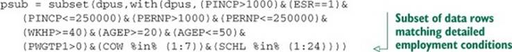
We don’t want to concentrate too much on this data; our goal is only to illustrate the modeling procedure. Conclusions are very dependent on choices of data conditioning (what subset of the data you use) and data coding (how you map records to informative symbols). This is why empirical scientific papers have a mandatory “materials and methods” section describing how data was chosen and prepared. Our data treatment is to select a subset of “typical full-time workers” by restricting the subset to data that meets all of the following conditions:
· Workers self-described as full-time employees
· Workers reporting at least 40 hours a week of activity
· Workers 20–50 years of age
· Workers with an annual income between $1,000 and $250,000 dollars
The following listing shows the code to limit to our desired subset of the data.
Listing 2.12. Selecting a subset of the Census data
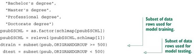
Recoding the data
Before we work with the data, we’ll recode some of the variables for readability. In particular, we want to recode variables that are enumerated integers into meaningful factor-level names, but for readability and to prevent accidentally treating such variables as mere numeric values. Listing 2.13 shows the typical steps needed to perform a useful recoding.
Listing 2.13. Recoding variables
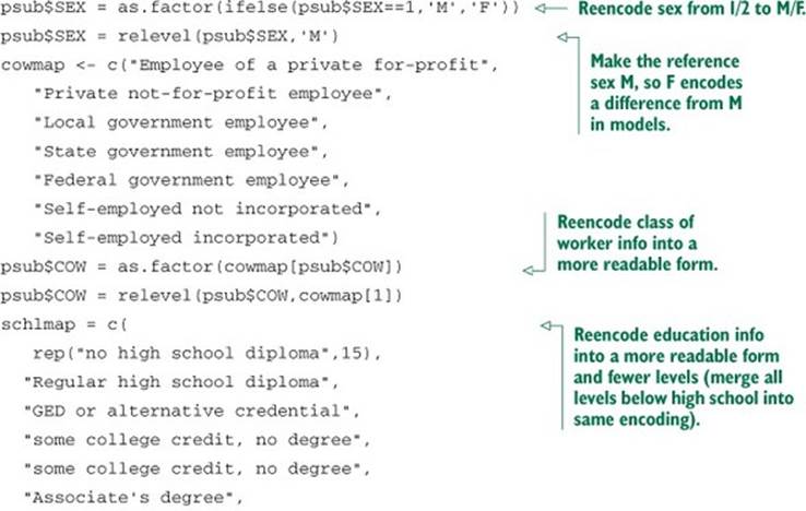
The data preparation is making use of R’s vectorized lookup operator []. For details on this or any other R commands, we suggest using the R help() command and appendix A (for help with [], type help('[')).
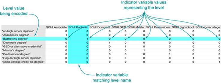
The standard trick to work with variables that take on a small number of string values is to reencode them into what’s called a factor as we’ve done with the as.factor() command. A factor is a list of all possible values of the variable (possible values are called levels), and each level works (under the covers) as an indicator variable. An indicator is a variable with a value of 1 (one) when a condition we’re interested in is true, and 0 (zero) otherwise. Indicators are a useful encoding trick. For example, SCHL is reencoded as 8 indicators with the names shown in figure 7.6 inchapter 7, plus the undisplayed level “no high school diploma.” Each indicator takes a value of 0, except when the SCHL variable has a value equal to the indicator’s name. When the SCHL variable matches the indicator name, the indicator is set to 1 to indicate the match. Figure 2.4 illustrates the process. SEX and COW underwent similar transformations.
Figure 2.4. Strings encoded as indicators
Examining the PUMS data
At this point, we’re ready to do some science, or at least start looking at the data. For example, we can quickly tabulate the distribution of category of work.
Listing 2.14. Summarizing the classifications of work
> summary(dtrain$COW)
Employee of a private for-profit Federal government employee
423 21
Local government employee Private not-for-profit employee
39 55
Self-employed incorporated Self-employed not incorporated
17 16
State government employee
24
Watch out for NAs
R’s representation for blank or missing data is NA. Unfortunately a lot of R commands quietly skip NAs without warning. The command table(dpus$COW,useNA='always') will show NAs much like summary(dpus$COW) does.
We’ll return to the Census example and demonstrate more sophisticated modeling techniques in chapter 7.
2.3. Summary
In this chapter, we’ve shown how to extract, transform, and load data for analysis. For smaller datasets we perform the transformations in R, and for larger datasets we advise using a SQL database. In either case we save all of the transformation steps as code (either in SQL or in R) that can be reused in the event of a data refresh. The whole purpose of this chapter is to prepare for the actual interesting work in our next chapters: exploring, managing, and correcting data.
The whole point of loading data into R is so we can start to work with it: explore, examine, summarize, and plot it. In chapter 3, we’ll demonstrate how to characterize your data through summaries, exploration, and graphing. These are key steps early in any modeling effort because it is through these steps that you learn the actual details and nature of the problem you’re hoping to model.
Key takeaways
· Data frames are your friend.
· Use read_table() to load small, structured datasets into R.
· You can use a package like RJDBC to load data into R from relational databases, and to transform or aggregate the data before loading using SQL.
· Always document data provenance.