Practical Data Science with R (2014)
Part 3. Delivering results
In part 2, we covered how to build a model that addresses the problem that you want to solve. The next steps are to implement your solution and communicate your results to other interested parties. In part 3, we conclude with the important steps of deploying work into production, documenting work, and building effective presentations.
Chapter 10 covers the documentation necessary for sharing or transferring your work to others, in particular those who will be deploying your model in an operational environment. This includes effective code commenting practices, as well as proper version management and collaboration with the version control software, git. We also discuss the practice of reproducible research using knitr. Chapter 10 also covers how to export models you’ve built from R, or deploy them as HTTP services.
Chapter 11 discusses how to present the results of your projects to different audiences. Project sponsors, project consumers (people in the organization who’ll be using or interpreting the results of your model), and fellow data scientists will all have different perspectives and interests. Inchapter 11, we give examples of how to tailor your presentations to the needs and interests of a specific audience.
On completing part 3, you’ll understand how to document and transfer the results of your project and how to effectively communicate your findings to other interested parties.
Chapter 10. Documentation and deployment
This chapter covers
· Producing effective milestone documentation
· Managing project history using source control
· Deploying results and making demonstrations
In this chapter, we’ll work through producing effective milestone documentation, code comments, version control records, and demonstration deployments. The idea is that these can all be thought of as important documentation of the work you’ve done. Table 10.1 expands a bit on our goals for this chapter.
Table 10.1. Chapter goals
|
Goal |
Description |
|
Produce effective milestone documentation |
A readable summary of project goals, data provenance, steps taken, and technical results (numbers and graphs). Milestone documentation is usually read by collaborators and peers, so it can be concise and can often include actual code. We’ll demonstrate a great tool for producing excellent milestone documentation: the R knitrpackage. knitr is a product of the “reproducible research” movement (see Christopher Gandrud’s Reproducible Research with R and RStudio, Chapman and Hall, 2013) and is an excellent way to produce a reliable snapshot that not only shows the state of a project, but allows others to confirm the project works. |
|
Manage a complete project history |
It makes little sense to have exquisite milestone or checkpoint documentation of how your project worked last February if you can’t get a copy of February’s code and data. This is why you need a good version control discipline. |
|
Deploy demonstrations |
True production deployments are best done by experienced engineers. These engineers know the tools and environment they will be deploying to. A good way to jump-start production deployment is to have a reference deployment. This allows engineers to experiment with your work, test corner cases, and build acceptance tests. |
This chapter explains how to share your work. We’ll discuss how to use knitr to create substantial project milestone documentation and automate reproduction of graphs and other results. You’ll learn about using effective comments in code, and using Git for version management and for collaboration. We’ll also discuss deploying models as HTTP services and exporting model results.
10.1. The buzz dataset
Our example dataset for this and the following chapter is the buzz dataset from http://ama.liglab.fr/datasets/buzz/. We’ll work with the data found in TomsHardware-Relative-Sigma-500.data.txt.[1] The original supplied documentation (TomsHardware-Relative-Sigma-500.names.txt and BuzzDataSetDoc.pdf) tells us the buzz data is structured as shown in table 10.2.
1 All files mentioned in this chapter are available from https://github.com/WinVector/zmPDSwR/tree/master/Buzz.
Table 10.2. Buzz data description
|
Attribute |
Description |
|
Rows |
Each row represents many different measurements of the popularity of a technical personal computer discussion topic. |
|
Topics |
Topics include technical issues about personal computers such as brand names, memory, overclocking, and so on. |
|
Measurement types |
For each topic, measurement types are quantities such as the number of discussions started, number of posts, number of authors, number of readers, and so on. Each measurement is taken at eight different times. |
|
Times |
The eight relative times are named 0 through 7 and are likely days (the original variable documentation is not completely clear and the matching paper has not yet been released). For each measurement type all eight relative times are stored in different columns in the same data row. |
|
Buzz |
The quantity to be predicted is called buzz and is defined as being true or 1 if the ongoing rate of additional discussion activity is at least 500 events per day averaged over a number of days after the observed days. Likely buzz is a future average of the seven variables labeled NAC (the original documentation is unclear on this). |
In our initial buzz documentation, we list what we know (and, importantly, admit what we’re not sure about). We don’t intend any disrespect in calling out issues in the supplied buzz documentation. That documentation is about as good as you see at the beginning of a project. In an actual project, you’d clarify and improve unclear points through discussions and work cycles. This is one reason having access to active project sponsors and partners is critical in real-world projects.
The buzz problem demonstrates some features that are common in actual data science projects:
· This is a project where we’re trying to predict the future from past features. These sorts of projects are particularly desirable, as we can expect to produce a lot of training data by saving past measurements.
· The quantity to be predicted is a function of future values of variables we’re measuring. So part of the problem is relearning the business rules that make the determination. In such cases, it may be better to steer the project to predict estimates of the future values in question and leave the decision rules to the business.
· A domain-specific reshaping of the supplied variables would be appropriate. We’re given daily popularities of articles over eight days; we’d prefer variables that represent popularity summed over the measured days, variables that measure topic age, variables that measure shape (indicating topics that are falling off fast or slow), and other time series–specific features.
In this chapter, we’ll use the buzz dataset as-is and concentrate on demonstrating the tools and techniques used in producing documentation, deployments, and presentations. In actual projects, we advise you to start by producing notes like those in table 10.2. You’d also incorporate meeting notes to document your actual project goals. As this is only a demonstration, we’ll emphasize technical documentation: data provenance and an initial trivial analysis to demonstrate we have control of the data. Our example initial buzz analysis is found here:https://github.com/WinVector/zmPDSwR/blob/master/Buzz/buzzm.md.[2] We suggest you skim it before we work through the tools and steps used to produce these documents in our next section.
2 Also available in PDF form: https://github.com/WinVector/zmPDSwR/raw/master/Buzz/buzz.pdf.
10.2. Using knitr to produce milestone documentation
The first audience you’ll have to prepare documentation for is yourself and your peers. You may need to return to previous work months later, and it may be in an urgent situation like an important bug fix, presentation, or feature improvement. For self/peer documentation, you want to concentrate on facts: what the stated goals were, where the data came from, and what techniques were tried. You assume as long as you use standard terminology or references that the reader can figure out anything else they need to know. You want to emphasize any surprises or exceptional issues, as they’re exactly what’s expensive to relearn. You can’t expect to share this sort of documentation with clients, but you can later use it as a basis for building wider documentation and presentations.
The first sort of documentation we recommend is project milestone or checkpoint documentation. At major steps of the project you should take some time out to repeat your work in a clean environment (proving you know what’s in intermediate files and you can in fact recreate them). An important, and often neglected, milestone is the start of a project. In this section, we’ll use the knitr R package to document starting work with the buzz data.
10.2.1. What is knitr?
knitr is an R package that allows the inclusion of R code and results inside documents. knitr’s operation is similar in concept to Knuth’s literate programming and to the R Sweave package. In practice you maintain a master file that contains both user-readable documentation and chunks of program source code. The document types supported by knitr include LaTeX, Markdown, and HTML. LaTeX format is a good choice for detailed typeset technical documents. Markdown format is a good choice for online documentation and wikis. Direct HTML format may be appropriate for some web applications.
knitr’s main operation is called a knit: knitr extracts and executes all of the R code and then builds a new result document that assembles the contents of the original document plus pretty-printed code and results (see figure 10.1).
Figure 10.1. knitr process schematic
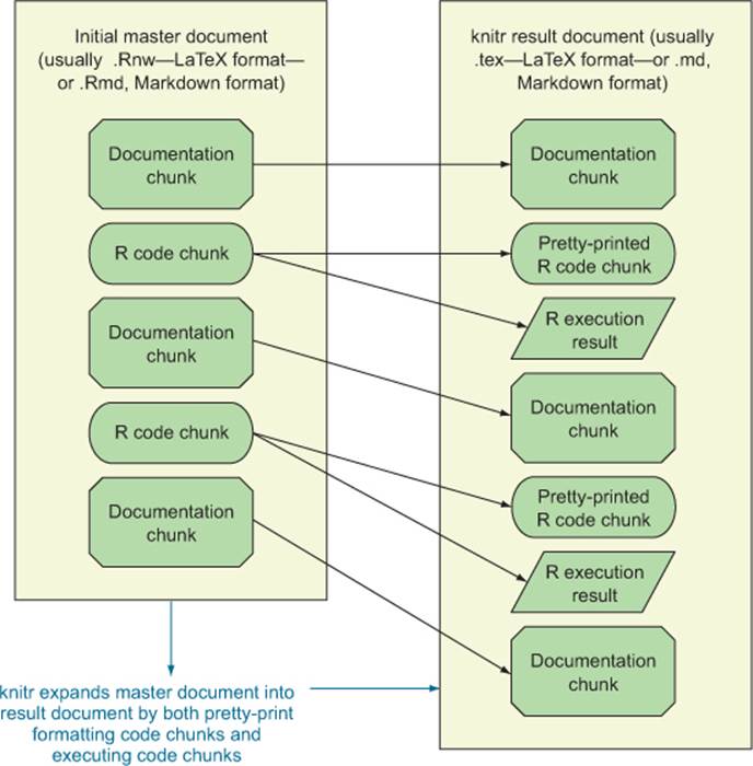
The process is best demonstrated with a few examples.
A simple knitr Markdown example
Markdown (http://daringfireball.net/projects/markdown/) is a simple web-ready format that’s used in many wikis. The following listing shows a simple Markdown document with knitr annotation blocks denoted with ```.
Listing 10.1. knitr-annotated Markdown
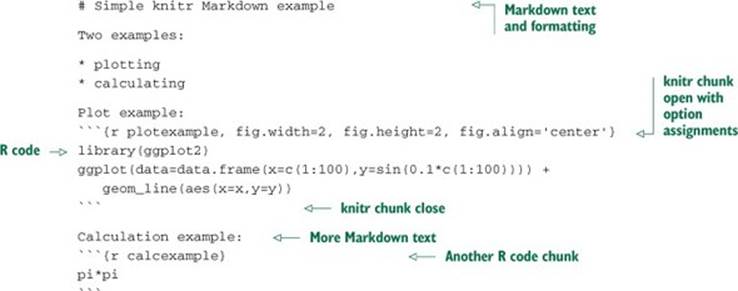
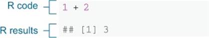
We’ll save listing 10.1 in a file named simple.Rmd. In R we’d process this as shown next:
library(knitr)
knit('simple.Rmd')
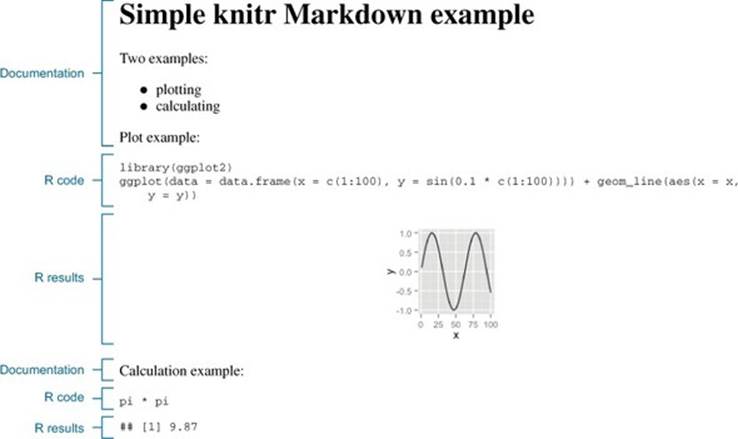
This produces the new file simple.md, which is in Markdown format and appears (with the proper viewer) as in figure 10.2.[3]
3 We used pandoc -o simple.html simple.md to convert the file to easily viewable HTML.
Figure 10.2. Simple knitr Markdown result
A simple knitr LaTeX example
LaTeX is a powerful document preparation system suitable for publication-quality typesetting both for articles and entire books. To show how to use knitr with LaTeX, we’ll work through a simple example. The main new feature is that in LaTeX, code blocks are marked with << and @ instead of ```. A simple LaTeX document with knitr chunks looks like the following listing.
Listing 10.2. knitr LaTeX example
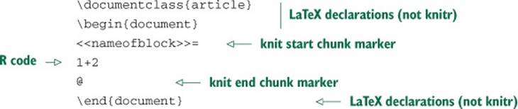
We’ll save this content into a file named add.Rnw and then (using the Bash shell) run R in batch to produce the file add.tex. At a shell prompt, we then run LaTeX to create the final add.pdf file:
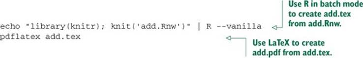
This produces the PDF as shown in figure 10.3.
Figure 10.3. Simple knitr LaTeX result
Purpose of knitr
The purpose of knitr is to produce reproducible work.[4] When you distribute your work in knitr format (as we do in section 10.2.3), anyone can download your work and, without great effort, rerun it to confirm they get the same results you did. This is the ideal standard of scientific research, but is rarely met, as scientists usually are deficient in sharing all of their code, data, and actual procedures. knitr collects and automates all the steps, so it becomes obvious if something is missing or doesn’t actually work as claimed. knitr automation may seem like a mere convenience, but it makes the essential work listed in table 10.3 much easier (and therefore more likely to actually be done).
4 The knitr community calls this reproducible research, but that’s because scientific work is often called research.
Table 10.3. Maintenance tasks made easier by knitr
|
Task |
Discussion |
|
Keeping code in sync with documentation |
With only one copy of the code (already in the document), it’s not so easy to get out of sync. |
|
Keeping results in sync with data |
Eliminating all by-hand steps (such as cutting and pasting results, picking filenames, and including figures) makes it much more likely you’ll correctly rerun and recheck your work. |
|
Handing off correct work to others |
If the steps are sequenced so a machine can run them, then it’s much easier to rerun and confirm them. Also, having a container (the master document) to hold all your work makes managing dependencies much easier. |
10.2.2. knitr technical details
To use knitr on a substantial project, you need to know more about how knitr code chunks work. In particular you need to be clear how chunks are marked and what common chunk options you’ll need to manipulate.
knitr block declaration format
In general, a knitr code block starts with the block declaration (``` in Markdown and << in LaTeX). The first string is the name of the block (must be unique across the entire project). After that, a number of comma-separated option=value chunk option assignments are allowed.
knitr chunk options
A sampling of useful option assignments is given in table 10.4.
Table 10.4. Some useful knitr options
|
Option name |
Purpose |
|
cache |
Controls whether results are cached. With cache=F (the default), the code chunk is always executed. With cache=T, the code chunk isn’t executed if valid cached results are available from previous runs. Cached chunks are essential when you’re revising knitr documents, but you should always delete the cache directory (found as a subdirectory of where you’re using knitr) and do a clean rerun to make sure your calculations are using current versions of the data and settings you’ve specified in your document. |
|
echo |
Controls whether source code is copied into the document. With echo=T (the default), pretty formatted code is added to the document. With echo=F, code isn’t echoed (useful when you only want to display results). |
|
eval |
Controls whether code is evaluated. With eval=T (the default), code is executed. With eval=F, it’s not (useful for displaying instructions). |
|
message |
Set message=F to direct R message() commands to the console running R instead of to the document. This is useful for issuing progress messages to the user that you don’t want in the final document. |
|
results |
Controls what’s to be done with R output. Usually you don’t set this option and output is intermingled (with ## comments) with the code. A useful option is results='hide', which suppresses output. |
|
tidy |
Controls whether source code is reformatted before being printed. You almost always want to set tidy=F, as the current version of knitr often breaks code due to mishandling of R comments when reformatting. |
Most of these options are demonstrated in our buzz example, which we’ll work through in the next section.
10.2.3. Using knitr to document the buzz data
For a more substantial example, we’ll use knitr to document the initial data treatment and initial trivial model for the buzz data (recall from section 10.1 that buzz is records of computer discussion topic popularity). We’ll produce a document that outlines the initial steps of working with the buzz data (the sorts of steps we had, up until now, been including in this book whenever we introduce a new dataset). This example works through advanced knitr topics such as caching (to speed up reruns), messages (to alert the user), and advanced formatting. We supply two examples of knitr for the buzz data at https://github.com/WinVector/zmPDSwR/tree/master/Buzz. The first example is in Markdown format and found in the knitr file buzzm.Rmd, which knits to the Markdown file buzzm.md. The second example is in LaTeX format and found in the knitr file buzz.Rnw, which knits to the LaTeX file buzz.tex (which in turn is used to produce the viewable file buzz.pdf). All steps we’ll mention in this section are completely demonstrated in both of these files. We’ll show excerpts from buzz.Rmd (using the ``` delimiter) and excerpts from buzz.Rnw (using the<< delimiter).
Buzz data notes
For the buzz data, the preparation notes can be found in the files buzz.md, buzz.html, or buzz.pdf. We suggest viewing one of these files and table 10.2. The original description files from the buzz project (Toms-Hardware-Relative-Sigma-500.names.txt and BuzzDataSetDoc.pdf) are also available at https://github.com/WinVector/zmPDSwR/tree/master/Buzz.
Setting up chunk cache dependencies
For a substantial knitr project, you’ll want to enable caching. Otherwise, rerunning knitr to correct typos becomes prohibitively expensive. The standard way to enable knitr caching is to add the cache=T option to all knitr chunks. You’ll also probably want to set up the chunk cache dependency calculator by inserting the following invisible chunk toward the top of your file.
Listing 10.3. Setting knitr dependency options
% set up caching and knitr chunk dependency calculation
% note: you will want to do clean re-runs once in a while to make sure
% you are not seeing stale cache results.
<<setup,tidy=F,cache=F,eval=T,echo=F,results='hide'>>=
opts_chunk$set(autodep=T)
dep_auto()
@
Confirming data provenance
Because knitr is automating steps, you can afford to take a couple of extra steps to confirm the data you’re analyzing is in fact the data you thought you had. For example, we’ll start our buzz data analysis by confirming that the SHA cryptographic hash of the data we’re starting from matches what we thought we had downloaded. This is done (assuming your system has the sha cryptographic hash installed) as shown in the following listing (note: always look to the first line of chunks for chunk options such as cache=T).
Listing 10.4. Using the system() command to compute a file hash
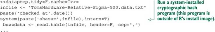
This code sequence depends on a program named "shasum" being on your execution path. You have to have a cryptographic hash installed, and you can supply a direct path to the program if necessary. Common locations for a cryptographic hash include /usr/bin/shasum, /sbin/md5, and fciv.exe, depending on your actual system configuration.
This code produces the output shown in figure 10.4. In particular, we’ve documented that the data we loaded has the same cryptographic hash we recorded when we first downloaded the data. Having confidence you’re still working with the exact same data you started with can speed up debugging when things go wrong. Note that we’re using the cryptographic hash to defend only against accident (using the wrong version of a file or seeing a corrupted file) and not to defend against true adversaries, so it’s okay to use a cryptographic hash that’s convenient even if it’s becoming out of date.
Figure 10.4. knitr documentation of buzz data load
Recording the performance of the naive analysis
The initial milestone is a good place to try to record the results of a naive “just apply a standard model to whatever variables are present” analysis. For the buzz data analysis, we’ll use a random forest modeling technique (not shown here, but in our knitr documentation) and apply the model to test data.
Listing 10.5. Calculating model performance
rtest <- data.frame(truth=buzztest$buzz,
pred=predict(fmodel, newdata=buzztest))
print(accuracyMeasures(rtest$pred, rtest$truth))
## [1] "precision= 0.809782608695652 ; recall= 0.84180790960452"
## pred
## truth 0 1
## 0 579 35
## 1 28 149
## model accuracy f1 dev.norm
## 1 model 0.9204 0.6817 4.401
Using milestones to save time
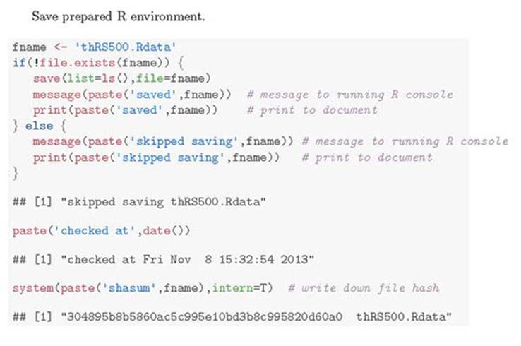
Now that we’ve gone to all the trouble to implement, write up, and run the buzz data preparation steps, we’ll end our knitr analysis by saving the R workspace. We can then start additional analyses (such as introducing better shape features for the time-varying data) from the saved workspace. In the following listing, we’ll show a conditional saving of the data (to prevent needless file churn) and again produce a cryptographic hash of the file (so we can confirm work that starts from a file with the same name is in fact starting from the same data).
Listing 10.6. Conditionally saving a file
Save prepared R environment.
% Another way to conditionally save, check for file.
% message=F is letting message() calls get routed to console instead
% of the document.
<<save,tidy=F,cache=F,message=F,eval=T>>=
fname <- 'thRS500.Rdata'
if(!file.exists(fname)) {
save(list=ls(),file=fname)
message(paste('saved',fname)) # message to running R console
print(paste('saved',fname)) # print to document
} else {
message(paste('skipped saving',fname)) # message to running R console
print(paste('skipped saving',fname)) # print to document
}
paste('checked at',date())
system(paste('shasum',fname),intern=T) # write down file hash
@
Figure 10.5 shows the result. The data scientists can safely start their analysis on the saved workspace and have documentation that allows them to confirm that a workspace file they’re using is in fact one produced by this version of the preparation steps.
Figure 10.5. knitr documentation of prepared buzz workspace
knitr takeaway
In our knitr example, we worked through the steps we’ve done for every dataset in this book: load data, manage columns/variables, perform an initial analysis, present results, and save a workspace. The key point is that because we took the extra effort to do this work in knitr, we have the following:
· Nicely formatted documentation (buzz.md and buzz.pdf)
· Shared executable code (buzz.Rmd and buzz.Rnw)
This makes debugging (which usually involves repeating and investigating earlier work), sharing, and documentation much easier and more reliable.
10.3. Using comments and version control for running documentation
Another essential record of your work is what we call running documentation. Running documentation is more informal than milestone/checkpoint documentation and is easiest maintained in the form of code comments and version control records. Undocumented, untracked code runs up a great deal of technical debt (see http://mng.bz/IaTd) that can cause problems down the road.
In this section, we’ll work through producing effective code comments and using Git for version control record keeping.
10.3.1. Writing effective comments
R’s comment style is simple: everything following a # (that isn’t itself quoted) until the end of a line is a comment and ignored by the R interpreter. The following listing is an example of a well-commented block of R code.
Listing 10.7. Example code comment
# Return the pseudo logarithm of x, which is close to
# sign(x)*log10(abs(x)) for x such that abs(x) is large
# and doesn't "blow up" near zero. Useful
# for transforming wide-range variables that may be negative
# (like profit/loss).
# See: http://www.win-vector.com/blog
# /2012/03/modeling-trick-the-signed-pseudo-logarithm/
# NB: This transform has the undesirable property of making most
# signed distributions appear bimodal around the origin, no matter
# what the underlying distribution really looks like.
# The argument x is assumed be numeric and can be a vector.
pseudoLog10 <- function(x) { asinh(x/2)/log(10) }
Good comments include what the function does, what types arguments are expected to be, limits of domain, why you should care about the function, and where it’s from. Of critical importance are any NB (nota bene or note well) or TODO notes. It’s vastly more important to document any unexpected features or limitations in your code than to try to explain the obvious. Because R variables don’t have types (only objects they’re pointing to have types), you may want to document what types of arguments you’re expecting. It’s critical to know if a function works correctly on lists, data frame rows, vectors, and so on.
Note that in our comments we didn’t bother with anything listed in table 10.5.
Table 10.5. Things not to worry about in comments
|
Item |
Why not to bother |
|
Pretty ASCII-art formatting |
It’s enough that the comment be there and be readable. Formatting into a beautiful block just makes the comment harder to maintain and decreases the chance of the comment being up to date. |
|
Anything we see in the code itself |
There’s no point repeating the name of the function, saying it takes only one argument, and so on. |
|
Anything we can get from version control |
We don’t bother recording the author or date the function was written. These facts, though important, are easily recovered from your version control system with commands like git blame. |
|
Any sort of Javadoc/ Doxygen-style annotations |
The standard way to formally document R functions is in separate .Rd (R documentation) files in a package structure (see http://cran.r-project.org/doc/manuals/R-exts.html). In our opinion, the R package system is too specialized and toilsome to use in regular practice (though it’s good for final delivery). For formal code documentation, we recommend knitr. |
Also, avoid comments that add no actual content, such as in the following listing.
Listing 10.8. Useless comment
#######################################
# Function: addone
# Author: John Mount
# Version: 1.3.11
# Location: RSource/helperFns/addone.R
# Date: 10/31/13
# Arguments: x
# Purpose: Adds one
#######################################
addone <- function(x) { x + 1 }
The only thing worse than no documentation is documentation that’s wrong. At all costs avoid comments that are incorrect, as in listing 10.9 (the comment says “adds one” when the code clearly adds two)—and do delete such comments if you find them.
Listing 10.9. Worse than useless comment
# adds one
addtwo <- function(x) { x + 2 }
10.3.2. Using version control to record history
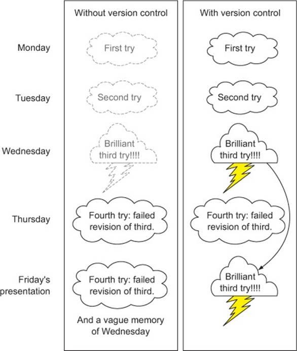
Version control can both maintain critical snapshots of your work in earlier states and produce running documentation of what was done by whom and when in your project. Figure 10.6 shows a cartoon “version control saves the day” scenario that is in fact common.
Figure 10.6. Version control saving the day
In this section, we’ll explain the basics of using Git (http://git-scm.com/) as a version control system. To really get familiar with Git, we recommend a good book such as Jon Loeliger and Matthew McCullough’s Version Control with Git, 2nd Edition (O’Reilly, 2012). Or, better yet, work with people who know Git. In this chapter, we assume you know how to run an interactive shell on your computer (on Linux and OS X you tend to use bash as your shell; on Windows you can install Cygwin—http://www.cygwin.com).
Working in bright light
Sharing your Git repository means you’re sharing a lot of information about your work habits and also sharing your mistakes. You’re much more exposed than when you just share final work or status reports. Make this a virtue: know you’re working in bright light. One of the most critical features in a good data scientist (perhaps even before analytic skill) is scientific honesty.
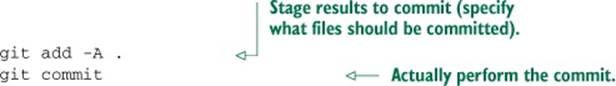
As a single user, to get most of the benefit from Git, you need to become familiar with a few commands:
· git init .
· git add -A .
· git commit
· git status
· git log
· git diff
· git checkout
Unfortunately, we don’t have space to explain all of these commands. We’ll demonstrate how to think about Git and the main path of commands you need to maintain your work history.
Choosing a project directory structure
Before starting with source control, it’s important to settle on and document a good project directory structure. Christopher Gandrud’s Reproducible Research with R and RStudio (Chapman & Hall, 2013) has good advice and instructions on how to do this. A pattern that’s worked well for us is to start a new project with the directory structure described in table 10.6.
Table 10.6. A possible project directory structure
|
Directory |
Description |
|
Data |
Where we save original downloaded data. This directory must usually be excluded from version control (using the .gitignore feature) due to file sizes, so you must ensure it’s backed up. We tend to save each data refresh in a separate subdirectory named by date. |
|
Scripts |
Where we store all code related to analysis of the data. |
|
Derived |
Where we store intermediate results that are derived from data and scripts. This directory must be excluded from source control. You also should have a master script that can rebuild the contents of this directory in a single command (and test the script from time to time). Typical contents of this directory are compressed files and file-based databases (H2, SQLite). |
|
Results |
Similar to derived, but this directory holds smaller later results (often based on derived) and hand-written content. These include important saved models, graphs, and reports. This directory is under version control, so collaborators can see what was said when. Any report shared with partners should come from this directory. |
Starting a Git project using the command line
When you’ve decided on your directory structure and want to start a version-controlled project, do the following:
1. Start the project in a new directory. Place any work either in this directory or in subdirectories.
2. Move your interactive shell into this directory and type git init .. It’s okay if you’ve already started working and there are already files present.
3. Exclude any subdirectories you don’t want under source control with .gitignore control files.
You can check if you’ve already performed the init step by typing git status. If the init hasn’t been done, you’ll get a message similar to fatal: Not a git repository (or any of the parent directories): .git.. If the init has been done, you’ll get a status message telling you something like on branch master and listing facts about many files.
The init step sets up in your directory a single hidden file tree called .git and prepares you to keep extra copies of every file in your directory (including subdirectories). Keeping all of these extra copies is called versioning and what is meant by version control. You can now start working on your project: save everything related to your work in this directory or some subdirectory of this directory.
Again, you only need to init a project once. Don’t worry about accidentally running git init . a second time; that’s harmless.
Using add/commit pairs to checkpoint work
As often as practical, enter the following two commands into an interactive shell in your project directory:
Get nervous about uncommitted state
A good rule of thumb for Git: you should be as nervous about having uncommitted changes as you should be about not having clicked Save. You don’t need to push/pull often, but you do need to make local commits often (even if you later squash them with a Git technique called rebasing).
Checking in a file is split into two stages: add and commit. This has some advantages (such as allowing you to inspect before committing), but for now just consider the two commands as always going together. The commit command should bring up an editor where you enter a comment as to what you’re up to. Until you’re a Git expert, allow yourself easy comments like “update,” “going to lunch,” “just added a paragraph,” or “corrected spelling.” Run the add/commit pair of commands after every minor accomplishment on your project. Run these commands every time you leave your project (to go to lunch, to go home, or to work on another project). Don’t fret if you forget to do this; just run the commands next time you remember.
A “wimpy commit” is better than no commit
We’ve been a little loose in our instructions to commit often and don’t worry too much about having a long commit message. Two things to keep in mind are that usually you want commits to be meaningful with the code working (so you tend not to commit in the middle of an edit with syntax errors), and good commit notes are to be preferred (just don’t forgo a commit because you don’t feel like writing a good commit note).
Using git log and git status to view progress
Any time you want to know about your work progress, type either git status to see if there are any edits you can put through the add/commit cycle, or git log to see the history of your work (from the viewpoint of the add/commit cycles).
The following listing shows the git status from our copy of this book’s examples repository (https://github.com/WinVector/zmPDSwR).
Listing 10.10. Checking your project status
$ git status
# On branch master
nothing to commit (working directory clean)
And the next listing shows a git log from the same project.
Listing 10.11. Checking your project history
commit c02839e0b34172f54fd68201f64895295b9d7609
Author: John Mount <jmount@win-vector.com>
Date: Sat Nov 9 13:28:30 2013 -0800
add export of random forest model
commit 974a8d5b95bdf25b95d23ef75d08d8aa6c0d74fe
Author: John Mount <jmount@win-vector.com>
Date: Sat Nov 9 12:01:14 2013 -0800
Add rook examples
The indented lines are the text we entered at the git commit step; the dates are tracked automatically.
Using Git through RStudio
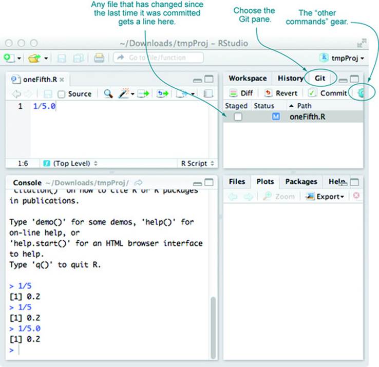
The RStudio IDE supplies a graphical user interface to Git that you should try. The add/commit cycle can be performed as follows in RStudio:
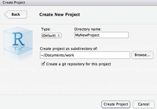
· Start a new project. From the RStudio command menu, select Project > Create Project, and choose New Project. Then select the name of the project, what directory to create the new project directory in, leave the type as (Default), and make sure Create a Git Repository for this Project is checked. When the new project pane looks something like figure 10.7, click Create Project, and you have a new project.
Figure 10.7. RStudio new project pane
· Do some work in your project. Create new files by selecting File > New > R Script. Type some R code (like 1/5) into the editor pane and then click the Save icon to save the file. When saving the file, be sure to choose your project directory or a subdirectory of your project.
· Commit your changes to version control. Figure 10.7 shows how to do this. Select the Git control pane in the top right of RStudio. This pane shows all changed files as line items. Check the Staged check box for any files you want to stage for this commit. Then click Commit, and you’re done.
You may not yet deeply understand or like Git, but you’re able to safely check in all of your changes every time you remember to stage and commit. This means all of your work history is there; you can’t clobber your committed work just by deleting your working file. Consider all of your working directory as “scratch work”—only checked-in work is safe from loss.
Your Git history can be seen by pulling down on the Other Commands gear (shown in the Git pane in figure 10.8) and selecting History (don’t confuse this with the nearby History pane, which is command history, not Git history). In an emergency, you can find Git help and find your earlier files. If you’ve been checking in, then your older versions are there; it’s just a matter of getting some help in accessing them. Also, if you’re working with others, you can use the push/pull menu items to publish and receive updates. Here’s all we want to say about version control at this point:commit often, and if you’re committing often, all problems can be solved with some further research. Also, be aware that since your primary version control is on your own machine, you need to make sure you have an independent backup of your machine. If your machine fails and your work hasn’t been backed up or shared, then you lose both your work and your version repository.
Figure 10.8. RStudio Git controls
10.3.3. Using version control to explore your project
Up until now, our model of version control has been this: Git keeps a complete copy of all of our files each time we successfully enter the pair of add/commit lines. We’ll now use these commits. If you add/commit often enough, Git is ready to help you with any of the following tasks:
· Tracking your work over time
· Recovering a deleted file
· Comparing two past versions of a file
· Finding when you added a specific bit of text
· Recovering a whole file or a bit of text from the past (undo an edit)
· Sharing files with collaborators
· Publicly sharing your project (à la GitHub at https://github.com/, or Bitbucket at https://bitbucket.org)
· Maintaining different versions (branches) of your work
And that’s why you want to add and commit often.
Getting help on Git
For any Git command, you can type git help [command] to get usage information. For example, to learn about git log, type git help log.
Finding out who wrote what and when
In section 10.3.1, we implied that a good version control system can produce a lot of documentation on its own. One powerful example is the command git blame. Look what happens if we download the Git repository https://github.com/WinVector/zmPDSwR (with the command git clone git@github.com:WinVector/zmPDSwR.git) and run the command git blame README.md.
Listing 10.12. Annoying work
git blame README.md
376f9bce (John Mount 2013-05-15 07:58:14 -0700 1) ## Support ...
376f9bce (John Mount 2013-05-15 07:58:14 -0700 2) # by Nina ...
2541bb0b (Marius Butuc 2013-04-24 23:52:09 -0400 3)
2541bb0b (Marius Butuc 2013-04-24 23:52:09 -0400 4) Works deri ...
2541bb0b (Marius Butuc 2013-04-24 23:52:09 -0400 5)
We’ve truncated lines for readability. But the git blame information takes each line of the file and prints the following:
· The prefix of the line’s Git commit hash. This is used to identify which commit the line we’re viewing came from.
· Who committed the line.
· When they committed the line.
· The line number.
· And, finally, the contents of the line.
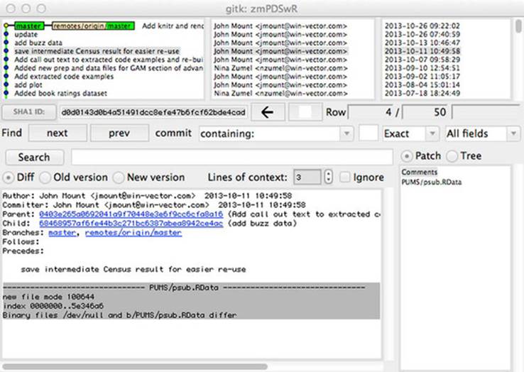
Viewing a detailed history of changes
The main ways to view the detailed history of your project are command-line tools like git log --graph --name-status and GUI tools such as RStudio and gitk. Continuing our https://github.com/WinVector/zmPDSwR example, we see the recent history of the repository by executing the git log command.
Listing 10.13. Viewing detailed project history
git log --graph --name-status
* commit c49c853cbcbb1e5a923d6e1127aa54ec7335d1b3
| Author: John Mount <jmount@win-vector.com>
| Date: Sat Oct 26 09:22:02 2013 -0700
|
| Add knitr and rendered result
|
| A Buzz/.gitignore
| A Buzz/buzz.Rnw
| A Buzz/buzz.pdf
|
* commit 6ce20dd33c5705b6de7e7f9390f2150d8d212b42
| Author: John Mount <jmount@win-vector.com>
| Date: Sat Oct 26 07:40:59 2013 -0700
|
| update
|
| M CodeExamples.zip
This variation of the git log command draws a graph of the history (mostly a straight line, which is the simplest possible history) and what files were added (the A lines), modified (the M lines), and so on. Commit comments are shown. Note that commit comments can be short. We can say things like “update” instead of “update Code-Examples.zip” because Git records what files were altered in each commit. The gitk GUI allows similar views and browsing through the detailed project history, as shown in figure 10.9.
Figure 10.9. gitk browsing https://github.com/WinVector/zmPDSwR
Using git diff to compare files from different commits
The git diff command allows you to compare any two committed versions of your project, or even to compare your current uncommitted work to any earlier version. In Git, commits are named using large hash keys, but you’re allowed to use prefixes of the hashes as names of commits.[5]For example, listing 10.14 demonstrates finding the differences in two versions of https://github.com/WinVector/zmPDSwR in a diff or patch format.
5 You can also create meaningful names for commits with the git tag command.
Listing 10.14. Finding line-based differences between two committed versions
diff --git a/CDC/NatalBirthData.rData b/CDC/NatalBirthData.rData
...
+++ b/CDC/prepBirthWeightData.R
@@ -0,0 +1,83 @@
+data <- read.table("natal2010Sample.tsv.gz",
+ sep="\t", header=T, stringsAsFactors=F)
+
+# make a boolean from Y/N data
+makevarYN = function(col) {
+ ifelse(col %in% c("", "U"), NA, ifelse(col=="Y", T, F))
+}
...
Try not to confuse Git commits and Git branches
A Git commit represents the complete state of a directory tree at a given time. A Git branch represents a sequence of commits and changes as you move through time. Commits are immutable; branches record progress.
Using git log to find the last time a file was around
After working on a project for a while, we often wonder, when did we delete a certain file and what was in it at the time? Git makes answering this question easy. We’ll demonstrate this in the repository https://github.com/WinVector/zmPDSwR. This repository has a README.md (Markdown) file, but we remember starting with a simple text file. When and how did that file get deleted? To find out, we’ll run the following (the command is after the $ prompt, and the rest of the text is the result):
$ git log --name-status -- README.txt
commit 2541bb0b9a2173eb1d471e11d4aca3b690a011ef
Author: Marius Butuc <marius.butuc@gmail.com>
Date: Wed Apr 24 23:52:09 2013 -0400
Translate readme to Markdown
D README.txt
commit 9534cff7579607316397cbb40f120d286b7e4b58
Author: John Mount <jmount@win-vector.com>
Date: Thu Mar 21 17:58:48 2013 -0700
update licenses
M README.txt
Ah—the file was deleted by Marius Butuc, an early book reader who generously composed a pull request to change our text file to Markdown (we reviewed and accepted the request at the time). We can view the contents of this older file with git show 9534cf -- README.txt (the9534cff is the prefix of the commit number before the deletion; manipulating these commit numbers isn’t hard if you use copy and paste). And we can recover that copy of the file with git checkout 9534cf -- README.txt.
10.3.4. Using version control to share work
In addition to producing work, you must often share it with peers. The common (and bad) way to do this is emailing zip files. Most of the bad sharing practices take excessive effort, are error-prone, and rapidly cause confusion. We advise using version control to share work with peers. To do that effectively with Git, you need to start using additional commands such as git pull, git rebase, and git push. Things seem more confusing at this point (though you still don’t need to worry about branching in its full generality), but are in fact far less confusing and less error-prone than ad hoc solutions. We almost always advise sharing work in star workflow, where each worker has their own repository, and a single common “naked” repository (a repository with only Git data structures and no ready-to-use files) is used to coordinate (thought of as a server or gold standard, often named origin).
The usual shared workflow is like this:
· Continuously: work, work, work.
· Frequently: commit results to the local repository using a git add/git commit pair.
· Every once in a while: pull a copy of the remote repository into our view with some variation of git pull and then use git push to push work upstream.
The main rule of Git is this: don’t try anything clever (push/pull, and so on) unless you’re in a “clean” state (everything committed, confirmed with git status).
Setting up remote repository relations
For two or more Git repositories to share work, the repositories need to know about each other through a relation called remote. A Git repository is able to share its work to a remote repository by the push command and pick up work from a remote repository by the pull command. Listing 10.15 shows the declared remotes for the authors’ local copy of the https://github.com/WinVector/zmPDSwR repository.
Listing 10.15. git remote
$ git remote --verbose
origin git@github.com:WinVector/zmPDSwR.git (fetch)
origin git@github.com:WinVector/zmPDSwR.git (push)
The remote relation is set when you create a copy of a repository using the git clone command or can be set using the git remote add command. In listing 10.15, the remote repository is called origin—this is the traditional name for a remote repository that you’re using as your master or gold standard. (Git tends not to use the name master for repositories because master is the name of the branch you’re usually working on.)
Using push and pull to synchronize work with remote repositories
Once your local repository has declared some other repository as remote, you can push and pull between the repositories. When pushing or pulling, always make sure you’re clean (have no uncommitted changes), and you usually want to pull before you push (as that’s the quickest way to spot and fix any potential conflicts). For a description of what version control conflicts are and how to deal with them, see http://mng.bz/5pTv.
Usually for simple tasks we don’t use branches (a technical version control term), and we use the rebase option on pull so that it appears that every piece of work is recorded into a simple linear order, even though collaborators are actually working in parallel. This is what we call anessential difficulty of working with others: time and order become separate ideas and become hard to track (and this is not a needless complexity added by using Git—there are such needless complexities, but this is not one of them).
The new Git commands you need to learn are these:
· git push (usually used in the git push -u origin master variation)
· git pull (usually used in the git fetch; git merge -m pull master origin/master or git pull --rebase origin master variations)
Typically two authors may be working on different files in the same project at the same time. As you can see in figure 10.10, the second author to push their results to the shared repository must decide how to specify the parallel work was performed. Either they can say the work was truly in parallel (represented by two branches being formed and then a merge record joining the work), or they can rebase their own work to claim their work was done “after” the other’s work (preserving a linear edit history and avoiding the need for any merge records). Note: before and after are tracked in terms of arrows, not time.
Figure 10.10. git pull: rebase versus merge
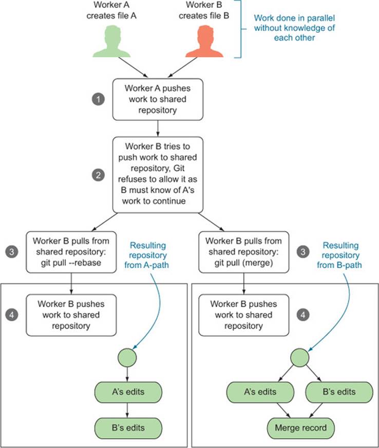
Merging is what’s really happening, but rebase is much simpler to read. The general rule is that you should only rebase work you haven’t yet shared (in our example, Worker B should feel free to rebase their edits to appear to be after Worker A’s edits, as Worker B hasn’t yet successfully pushed their work anywhere). You should avoid rebasing records people have seen, as you’re essentially hiding the edit steps they may be basing their work on (forcing them to merge or rebase in the future to catch up with your changed record keeping).
For most projects, we try to use a rebase-only strategy. For example, this book itself is maintained in a Git repository. We have only two authors who are in close proximity (so able to easily coordinate), and we’re only trying to create one final copy of the book (we’re not trying to maintain many branches for other uses). If we always rebase, the edit history will appear totally ordered (for each pair of edits, one is always recorded as having come before the other) and this makes talking about versions of the book much easier (again, before is determined by arrows in the edit history, not by time stamp).
Don’t confuse version control with backup
Git keeps multiple copies and records of all of your work. But until you push to a remote destination, all of these copies are on your machine in the .git directory. So don’t confuse basic version control with remote backups; they’re complementary.
A bit on the Git philosophy
Git is interesting in that it automatically detects and manages so much of what you’d have to specify with other version control systems (for example, Git finds which files have changed instead of you having to specify them, and Git also decides which files are related). Because of the large degree of automation, beginners usually severely underestimate how much Git tracks for them. This makes Git fairly quick except when Git insists you help decide how a possible global inconsistency should be recorded in history (either as a rebase or a branch followed by a merge record). The point is this: Git suspects possible inconsistency based on global state (even when the user may not think there is such) and then forces the committer to decide how to annotate the issue at the time of commit (a great service to any possible readers in the future). Git automates so much of the record-keeping that it’s always a shock when you have a conflict and have to express opinions on nuances you didn’t know were being tracked. Git is also an “anything is possible, but nothing is obvious or convenient” system. This is hard on the user at first, but in the end is much better than an “everything is smooth, but little is possible” version control system (which can leave you stranded).
Keep notes
Git commands are confusing; you’ll want to keep notes. One idea is to write a 3 × 5 card for each command you’re regularly using. Ideally you can be at the top of your Git game with about seven cards.
10.4. Deploying models
Good data science shares a rule with good writing: show, don’t tell. And a successful data science project should include at least a demonstration deployment of any techniques and models developed. Good documentation and presentation are vital, but at some point people have to see things working and be able to try their own tests. We strongly encourage partnering with a development group to produce the actual production-hardened version of your model, but a good demonstration helps recruit these collaborators.
We outline some deployment methods in table 10.7.
Table 10.7. Methods to demonstrate predictive model operation
|
Method |
Description |
|
Batch |
Data is brought into R, scored, and then written back out. This is essentially an extension of what you’re already doing with test data. |
|
Cross-language linkage |
R supplies answers to queries from another language (C, C++, Python, Java, and so on). R is designed with efficient cross-language calling in mind (in particular the Rcpp package), but this is a specialized topic we won’t cover here. |
|
Services |
R can be set up as an HTTP service to take new data as an HTTP query and respond with results. |
|
Export |
Often model evaluation is simple compared to model construction. In this case, the data scientist can export the model and a specification for the code to evaluate the model, and the production engineers can implement (with tests) model evaluation in the language of their choice (SQL, Java, C++, and so on). |
|
PMML |
PMML, or Predictive Model Markup Language, is a shared XML format that many modeling packages can export to and import from. If the model you produce is covered by R’s package pmml, you can export it without writing any additional code. Then any software stack that has an importer for the model in question can use your model. |
We’ve already demonstrated batch operation of models each time we applied a model to a test set. We won’t work through an R cross-language linkage example as it’s very specialized and requires knowledge of the system you’re trying to link to. We’ll demonstrate service and export strategies.
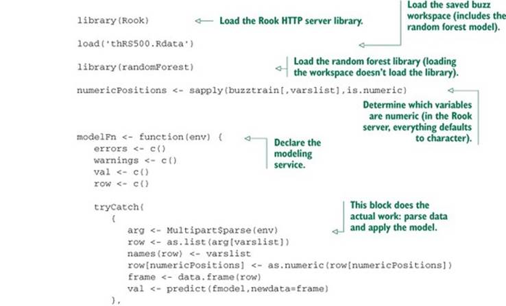
10.4.1. Deploying models as R HTTP services
One easy way to demonstrate an R model in operation is to expose it as an HTTP service. In the following listing, we show how to do this for our buzz model (predicting discussion topic popularity).
Listing 10.16. Buzz model as an R-based HTTP service
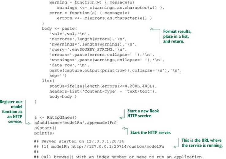
The next listing shows how to call the HTTP service.
Listing 10.17. Calling the buzz HTTP service

This produces the HTML form buzztest7.html, shown in figure 10.11 (also saved in our example GitHub repository).
Figure 10.11. Top of HTML form that asks server for buzz classification on submit
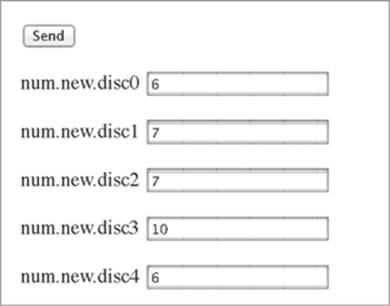
The generated file buzztest7.html contains a form element that has an action of "http://127.0.0.1:20714/custom/modelFn" as a POST. So when the Send button on this page is clicked, all the filled-out features are submitted to our server, and (assuming the form’s action is pointing to a valid server and port) we get a classification result from our model. This HTML query can be submitted from anywhere and doesn’t require R. An example result is saved in GitHub as buzztest7res.txt. Here’s an excerpt:
val=1
nerrors=0
nwarnings=0
...
Note that the result is a prediction of val=1, which was what we’d expect for the seventh row of the test data. The point is that the copy of R running the Rook server is willing to classify examples from any source. Such a server can be used as part of a larger demonstration and can allow non-R users to enter example data. If you were pushing this further, you could move to more machine-friendly formats such as JSON, but this is far enough for an initial demonstration.
10.4.2. Deploying models by export
Because training is often the hard part of building a model, it often makes sense to export a finished model for use by other systems. For example, a lot of theory goes into how a random forest picks variables and builds its trees. The structure of our random forest model is large but simple: a big collection of decision trees. But the construction is time-consuming and technical. The idea is this: it can be easier to fax a friend a solved Sudoku puzzle than to teach them your entire solution strategy.
So it often makes sense to export a copy of the finished model from R, instead of attempting to reproduce all of the details of model construction. When exporting a model, you’re depending on development partners to handle the hard parts of hardening a model for production (versioning, dealing with exceptional conditions, and so on). Software engineers tend to be good at project management and risk control, so export projects are also a good opportunity to learn.
The steps required depend a lot on the model and data treatment. For many models, you only need to save a few coefficients. For random forests, you need to export the trees. In all cases, you need to write code in your target system (be it SQL, Java, C, C++, Python, Ruby, and so on) to evaluate the model.[6]
6 A fun example is the Salford Systems Random Forests package that exports models as source code instead of data. The package creates a compilable file in your target language (often Java or C++) that implements the decision trees essentially as a series of if statements over class variables.
One of the issues of exporting models is that you must repeat any data treatment. So part of exporting a model is producing a specification of the data treatment (so it can be reimplemented outside of R).
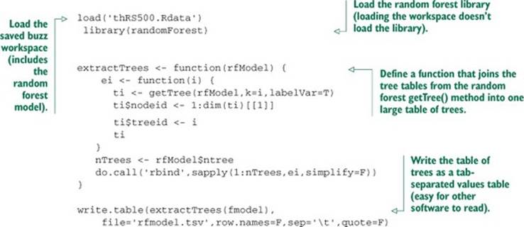
In listing 10.18, we show how to export the buzz random forest model. Some investigation of the random forest model and documentation showed that the underlying trees are accessible through a method called getTree(). In this listing, we combine the description of all of these trees into a single table.
Listing 10.18. Exporting the random forest model
A random forest model is a collection of decision trees, and figure 10.12 shows an extract of a single tree from the buzz random forest model. A decision tree is a series of tests traditionally visualized as a diagram of decision nodes, as shown in the top portion of the figure. The content of a decision tree is easy to store in a table where each table row represents the facts about the decision node (the variables being tested, the level of the test, and the IDs of the next nodes to go to, depending on the result of the test), as shown in the bottom part of the figure. To reimplement a random forest model, one just has to write code to accept the table representations of all the trees in the random forest model and trace through the specified tests.[7]
7 We’ve also saved the exported table here: https://github.com/WinVector/zmPDSwR/blob/master/Buzz/rfmodel.tsv.
Figure 10.12. One tree from the buzz random forest model

Your developer partners would then build tools to read the model trees and evaluate the trees on new data. Previous test results and demonstration servers become the basis of important acceptance tests.
10.4.3. What to take away
You should now be comfortable demonstrating R models to others. Of particular power is setting up a model as an HTTP service that can be experimented with by others, and also exporting models so model evaluation can be reimplemented in a production environment.
Always make sure your predictions in production are bounded
A secret trick of successful production deployments is to always make sure your predictions are bounded. This can prevent disasters in production. For a classification or probability problem (such as our buzz example), your predictions are automatically bounded between 0 and 1 (though there is some justification for adding code to tighten the allowed prediction region to between 1/n and 1-1/n for models built from n pieces of training data). For models that predict a value or score (such as linear regression), you almost always want to limit the predictions to be between themin and max values seen during training. This helps prevent a runaway input from driving your prediction to unprecedented (and unjustifiable) levels, possibly causing disastrous actions in production. You also want to signal when predictions have been so “touched up,” as unnoticed corrections can also be dangerous.
10.5. Summary
This chapter shared options on how to manage and share your work. In addition, we showed some techniques to set up demonstration HTTP services and export models for use by other software (so you don’t add R as a dependency in production).
Key takeaways
· Use knitr to produce significant reproducible milestone/checkpoint documentation.
· Write effective comments.
· Use version control to save your work history.
· Use version control to collaborate with others.
· Make your models available to your partners for experimentation and testing.
All materials on the site are licensed Creative Commons Attribution-Sharealike 3.0 Unported CC BY-SA 3.0 & GNU Free Documentation License (GFDL)
If you are the copyright holder of any material contained on our site and intend to remove it, please contact our site administrator for approval.
© 2016-2026 All site design rights belong to S.Y.A.