Practical Data Science with R (2014)

Part 2. Modeling methods

Chapter 9. Exploring advanced methods

This chapter covers

· Reducing training variance with bagging and random forests

· Learning non-monotone relationships with generalized additive models

· Increasing data separation with kernel methods

· Modeling complex decision boundaries with support vector machines

In the last few chapters, we’ve covered basic predictive modeling algorithms that you should have in your toolkit. These machine learning methods are usually a good place to start. In this chapter, we’ll look at more advanced methods that resolve specific weaknesses of the basic approaches. The main weaknesses we’ll address are training variance, non-monotone effects, and linearly inseparable data.

To illustrate the issues, let’s consider a silly health prediction model. Suppose we have for a number of patients (of widely varying but unrecorded ages) recorded height (as h in feet) and weight (as w in pounds), and an appraisal of “healthy” or “unhealthy.” The modeling question is this: can height and weight accurately predict health appraisal? Models built off such limited features provide quick examples of the following common weaknesses:

· Training variance— Training variance is when small changes in the makeup of the training set result in models that make substantially different predictions. Decision trees can exhibit this effect. Both bagging and random forests can reduce training variance and sensitivity to overfitting.

· Non-monotone effects— Linear regression and logistic regression (see chapter 7) both treat numeric variables in a monotone matter: if more of a quantity is good, then much more of the quantity is better. This is often not the case in the real world. For example, ideal healthy weight is in a bounded range, not arbitrarily heavy or arbitrarily light. Generalized additive models add the ability to model interesting variable effects and ranges to linear models and generalized linear models (such as logistic regression).

· Linearly inseparable data— Often the concept we’re trying to learn is not a linear combination of the original variables. Take BMI, or body mass index, for example: BMI purports to relate height (h) and weight (w) through the expression w/h² to health (rightly or wrongly). The termw/h² is not a linear combination of w and h, so neither linear regression or logistic regression would directly discover such a relation. It’s reasonable to expect that a model that has a term of w/h² could produce better predictions of health appraisal than a model that only has linear combinations of h and w. This is because the data is more “separable” with respect to a w/h²-shaped decision surface than to an h-shaped decision surface. Kernel methods allow the data scientist to introduce new nonlinear combination terms to models (like w/h²), and support vector machines (SVMs) use both kernels and training data to build useful decision surfaces.

These issues don’t always cause modeling efforts to visibly fail. Instead they often leave you with a model that’s not as powerful as it could be. In this chapter, we’ll use a few advanced methods to fix such modeling weaknesses lurking in earlier examples. We’ll start with a demonstration of bagging and random forests.

9.1. Using bagging and random forests to reduce training variance

In section 6.3.2, we looked at using decision trees for classification and regression. As we mentioned there, decision trees are an attractive method for a number of reasons:

· They take any type of data, numerical or categorical, without any distributional assumptions and without preprocessing.

· Most implementations (in particular, R’s) handle missing data; the method is also robust to redundant and nonlinear data.

· The algorithm is easy to use, and the output (the tree) is relatively easy to understand.

· Once the model is fit, scoring is fast.

On the other hand, decision trees do have some drawbacks:

· They have a tendency to overfit, especially without pruning.

· They have high training variance: samples drawn from the same population can produce trees with different structures and different prediction accuracy.

· Prediction accuracy can be low, compared to other methods.^[1]

¹ See Lim, Loh, and Shih, “A Comparison of Prediction Accuracy, Complexity, and Training Time of Thirty-three Old and New Classification Algorithms,” Machine Learning, 2000. 40, 203–229; online at http://mng.bz/rwKM.

For these reasons a technique called bagging is often used to improve decision tree models, and a more specialized approach called random forests directly combines decision trees with bagging. We’ll work examples of both techniques.

9.1.1. Using bagging to improve prediction

One way to mitigate the shortcomings of decision tree models is by bootstrap aggregation, or bagging. In bagging, you draw bootstrap samples (random samples with replacement) from your data. From each sample, you build a decision tree model. The final model is the average of all the individual decision trees.^[2] To make this concrete, suppose that x is an input datum, y_i(x) is the output of the ith tree, c(y_1(x), y_2(x), ... y_n(x)) is the vector of individual outputs, and y is the output of the final model:

² Bagging and random forests (which we’ll describe in the next section) are two variations of a general technique called ensemble learning. An ensemble model is composed of the combination of several smaller simple models (often small decision trees). Giovanni Seni and John Elder’s Ensemble Methods in Data Mining (Morgan & Claypool, 2010) is an excellent introduction to the general theory of ensemble learning.

· For regression, or for estimating class probabilities, y(x) is the average of the scores returned by the individual trees: y(x) = mean(c(y_1(x), ... y_n(x))).

· For classification, the final model assigns the class that got the most votes from the individual trees.

Bagging decision trees stabilizes the final model by lowering the variance; this improves the accuracy. A bagged ensemble of trees is also less likely to overfit the data.

Bagging classifiers

The proofs that bagging reduces variance are only valid for regression and for estimating class probabilities, not for classifiers (a model that only returns class membership, not class probabilities). Bagging a bad classifier can make it worse. So you definitely want to work over estimated class probabilities, if they’re at all available. But it can be shown that for CART trees (which is the decision tree implementation in R) under mild assumptions, bagging tends to increase classifier accuracy. See Clifton D. Sutton, “Classification and Regression Trees, Bagging, and Boosting,”Handbook of Statistics, Vol. 24 (Elsevier, 2005) for more details.

The Spambase dataset (also used in chapter 5) provides a good example of the bagging technique. The dataset consists of about 4,600 documents and 57 features that describe the frequency of certain key words and characters. First we’ll train a decision tree to estimate the probability that a given document is spam, and then we’ll evaluate the tree’s deviance (which you’ll recall from discussions in chapters 5 and 7 is similar to variance) and its prediction accuracy.

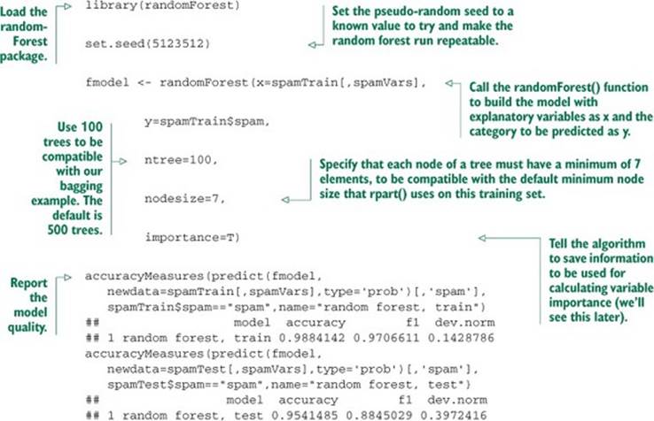
First, let’s load the data. As we did in section 5.2, let’s download a copy of spamD .tsv (https://github.com/WinVector/zmPDSwR/raw/master/Spambase/spamD.tsv). Then we’ll write a few convenience functions and train a decision tree, as in the following listing.

Listing 9.1. Preparing Spambase data and evaluating the performance of decision trees

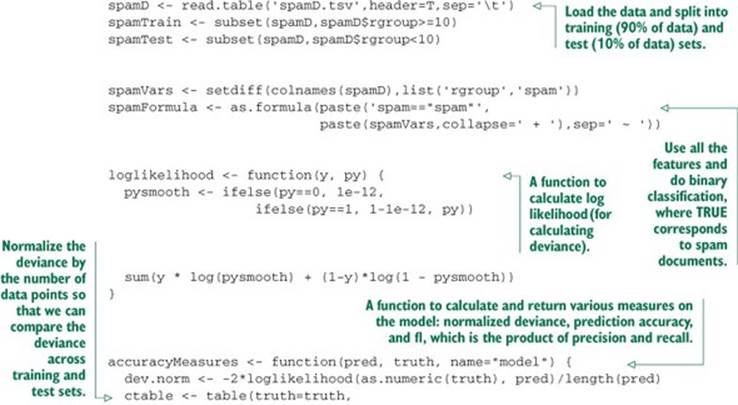
The output of the last two calls to accuracyMeasures() produces the following output. As expected, the accuracy and F1 scores both degrade on the test set, and the deviance increases (we want the deviance to be small):

model accuracy f1 dev.norm

tree, training 0.9104514 0.7809002 0.5618654

model accuracy f1 dev.norm

tree, test 0.8799127 0.7091151 0.6702857

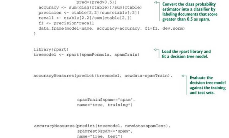
Now let’s try bagging the decision trees.

Listing 9.2. Bagging decision trees

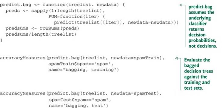
This results in the following:

model accuracy f1 dev.norm

bagging, training 0.9220372 0.8072953 0.4702707

model accuracy f1 dev.norm

bagging, test 0.9061135 0.7646497 0.528229

As you see, bagging improves accuracy and F1, and reduces deviance over both the training and test sets when compared to the single decision tree (we’ll see a direct comparison of the scores a little later on). The improvement is more dramatic on the test set: the bagged model has less generalization error^[3] than the single decision tree. We can further improve model performance by going from bagging to random forests.

³ Generalization error is the difference in accuracy of the model on data it’s never seen before, as compared to its error on the training set.

9.1.2. Using random forests to further improve prediction

In bagging, the trees are built using randomized datasets, but each tree is built by considering the exact same set of features. This means that all the individual trees are likely to use very similar sets of features (perhaps in a different order or with different split values). Hence, the individual trees will tend to be overly correlated with each other. If there are regions in feature space where one tree tends to make mistakes, then all the trees are likely to make mistakes there, too, diminishing our opportunity for correction. The random forest approach tries to de-correlate the trees by randomizing the set of variables that each tree is allowed to use. For each individual tree in the ensemble, the random forest method does the following:

1. Draws a bootstrapped sample from the training data

2. For each sample, grows a decision tree, and at each node of the tree

1. Randomly draws a subset of mtry variables from the p total features that are available

2. Picks the best variable and the best split from that set of mtry variables

3. Continues until the tree is fully grown

The final ensemble of trees is then bagged to make the random forest predictions. This is quite involved, but fortunately all done by a single-line random forest call.

By default, the randomForest() function in R draws mtry = p/3 variables at each node for regression trees and m = sqrt(p) variables for classification trees. In theory, random forests aren’t terribly sensitive to the value of mtry. Smaller values will grow the trees faster; but if you have a very large number of variables to choose from, of which only a small fraction are actually useful, then using a larger mtry is better, since with a larger mtry you’re more likely to draw some useful variables at every step of the tree-growing procedure.

Continuing from the data in section 9.1, let’s build a spam model using random forests.

Listing 9.3. Using random forests

Let’s summarize the results for all three of the models we’ve looked at:

# Performance on the training set

model accuracy f1 dev.norm

Tree 0.9104514 0.7809002 0.5618654

Bagging 0.9220372 0.8072953 0.4702707

Random Forest 0.9884142 0.9706611 0.1428786

# Performance on the test set

model accuracy f1 dev.norm

Tree 0.8799127 0.7091151 0.6702857

Bagging 0.9061135 0.7646497 0.5282290

Random Forest 0.9541485 0.8845029 0.3972416

# Performance change between training and test:

# The decrease in accuracy and f1 in the test set

# from training, and the increase in dev.norm

# in the test set from training.

# (So in every case, smaller is better)

model accuracy f1 dev.norm

Tree 0.03053870 0.07178505 -0.10842030

Bagging 0.01592363 0.04264557 -0.05795832

Random Forest 0.03426572 0.08615813 -0.254363

The random forest model performed dramatically better than the other two models in both training and test. But the random forest’s generalization error was comparable to that of a single decision tree (and almost twice that of the bagged model).^[4]

⁴ When a machine learning algorithm shows an implausibly good fit (like 0.99+ accuracy), it can be a symptom that you don’t have enough training data to falsify bad modeling alternatives. Limiting the complexity of the model can cut down on generalization error and overfitting and can be worthwhile, even if it decreases training performance.

Random forests can overfit!

It’s lore among random forest proponents that “random forests don’t overfit.” In fact, they can. Hastie et al. back up this observation in their chapter on random forests in The Elements of Statistical Learning, Second Edition (Springer, 2009). Look for unreasonably good fits on the training data as evidence of useless overfit and memorization. Also, it’s important to evaluate your model’s performance on a holdout set.

You can also mitigate the overfitting problem by limiting how deep the trees can be grown (using the maxnodes parameter to randomForest()). When you do this, you’re deliberately degrading model performance on training data so that you can more usefully distinguish between models and falsify bad training decisions.

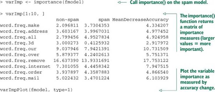
Examining variable importance

A useful feature of the randomForest() function is its variable importance calculation. Since the algorithm uses a large number of bootstrap samples, each data point x has a corresponding set of out-of-bag samples: those samples that don’t contain the point x. The out-of-bag samples can be used is a way similar to N-fold cross validation, to estimate the accuracy of each tree in the ensemble.

To estimate the “importance” of a variable v, the variable’s values are randomly permuted in the out-of-bag samples, and the corresponding decrease in each tree’s accuracy is estimated. If the average decrease over all the trees is large, then the variable is considered important—its value makes a big difference in predicting the outcome. If the average decrease is small, then the variable doesn’t make much difference to the outcome. The algorithm also measures the decrease in node purity that occurs from splitting on a permuted variable (how this variable affects the quality of the tree).

We can calculate the variable importance by setting importance=T in the randomForest() call, and then calling the functions importance() and varImpPlot().

Listing 9.4. randomForest variable importance()

The result of the varImpPlot() call is shown in figure 9.1.

Figure 9.1. Plot of the most important variables in the spam model, as measured by accuracy

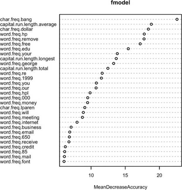
Knowing which variables are most important (or at least, which variables contribute the most to the structure of the underlying decision trees) can help you with variable reduction. This is useful not only for building smaller, faster trees, but for choosing variables to be used by another modeling algorithm, if that’s desired. We can reduce the number of variables in this spam example from 57 to 25 without affecting the quality of the final model.

Listing 9.5. Fitting with fewer variables

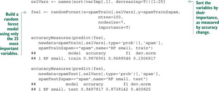
The smaller model performs just as well as the random forest model built using all 57 variables.

9.1.3. Bagging and random forest takeaways

Here’s what you should remember about bagging and random forests:

· Bagging stabilizes decision trees and improves accuracy by reducing variance.

· Bagging reduces generalization error.

· Random forests further improve decision tree performance by de-correlating the individual trees in the bagging ensemble.

· Random forests’ variable importance measures can help you determine which variables are contributing the most strongly to your model.

· Because the trees in a random forest ensemble are unpruned and potentially quite deep, there’s still a danger of overfitting. Be sure to evaluate the model on holdout data to get a better estimate of model performance.

Bagging and random forests are after-the-fact improvements we can try in order to improve model outputs. In our next section, we’ll work with generalized additive models, which work to improve how model inputs are used.

9.2. Using generalized additive models (GAMs) to learn non-monotone relationships

In chapter 7, we looked at how to use linear regression to model and predict quantitative output, and how to use logistic regression to predict class probabilities. Linear and logistic regression models are powerful tools, especially when you want to understand the relationship between the input variables and the output. They’re robust to correlated variables (when regularized), and logistic regression preserves the marginal probabilities of the data. The primary shortcoming of both these models is that they assume that the relationship between the inputs and the output is monotone. That is, if more is good, than much more is always better.

But what if the actual relationship is non-monotone? For example, for underweight patients, increasing weight can increase health. But there’s a limit: at some point more weight is bad. Linear and logistic regression miss this distinction (but still often perform surprisingly well, hiding the issue). Generalized additive models (GAMs) are a way to model non-monotone responses within the framework of a linear or logistic model (or any other generalized linear model).

9.2.1. Understanding GAMs

Recall that, if y[i] is the numeric quantity you want to predict, and x[i,] is a row of inputs that corresponds to output y[i], then linear regression finds a function f(x) such that

f(x[i,]) = b0 + b[1] x[i,1] + b[2] x[i,2] + ... b[n] x[i,n]

And f(x[i,]) is as close to y[i] as possible.

In its simplest form, a GAM model relaxes the linearity constraint and finds a set of functions s_i() (and a constant term a0) such that

f(x[i,]) = a0 + s_1(x[i,1]) + s_2(x[i,2]) + ... s_n(x[i,n])

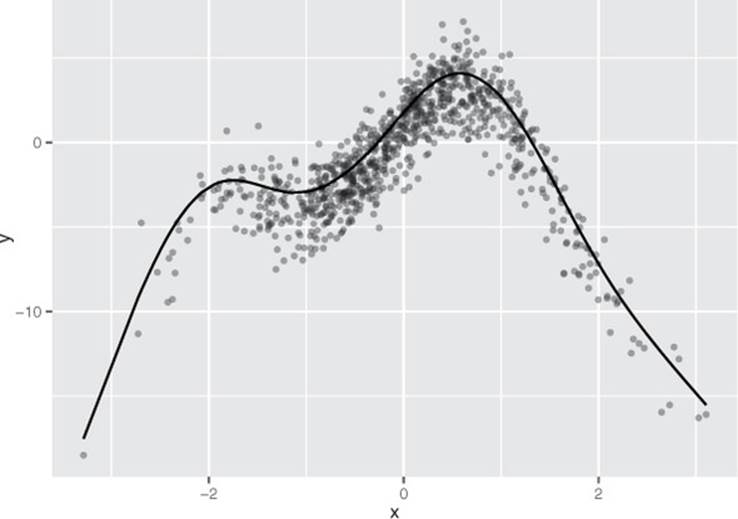
And f(x[i,]) is as close to y[i] as possible. The functions s_i() are smooth curve fits that are built up from polynomials. The curves are called splines and are designed to pass as closely as possible through the data without being too “wiggly” (without overfitting). An example of a spline fit is shown in figure 9.2.

Figure 9.2. A spline that has been fit through a series of points

Let’s work on a concrete example.

9.2.2. A one-dimensional regression example

Let’s consider a toy example where the response y is a noisy nonlinear function of the input variable x (in fact, it’s the function shown in figure 9.2). As usual, we’ll split the data into training and test sets.

Listing 9.6. Preparing an artificial problem

set.seed(602957)

x <- rnorm(1000)

noise <- rnorm(1000, sd=1.5)

y <- 3*sin(2*x) + cos(0.75*x) - 1.5*(x^2 ) + noise

select <- runif(1000)

frame <- data.frame(y=y, x = x)

train <- frame[select > 0.1,]

test <-frame[select <= 0.1,]

Given the data is from the nonlinear functions sin() and cos(), there shouldn’t be a good linear fit from x to y. We’ll start by building a (poor) linear regression.

Listing 9.7. Linear regression applied to our artificial example

> lin.model <- lm(y ~ x, data=train)

> summary(lin.model)

Call:

lm(formula = y ~ x, data = train)

Residuals:

Min 1Q Median 3Q Max

-17.698 -1.774 0.193 2.499 7.529

Coefficients:

Estimate Std. Error t value Pr(>|t|)

(Intercept) -0.8330 0.1161 -7.175 1.51e-12 ***

x 0.7395 0.1197 6.180 9.74e-10 ***

---

Signif. codes: 0 ’ ***’ 0.001 ’ **’ 0.01 ’ *’ 0.05 ’ .’ 0.1 ’ ’ 1

Residual standard error: 3.485 on 899 degrees of freedom

Multiple R-squared: 0.04075, Adjusted R-squared: 0.03968

F-statistic: 38.19 on 1 and 899 DF, p-value: 9.737e-10

#

# calculate the root mean squared error (rmse)

#

> resid.lin <- train$y-predict(lin.model)

> sqrt(mean(resid.lin^2))

[1] 3.481091

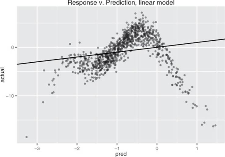
The resulting model’s predictions are plotted versus true response in figure 9.3. As expected, it’s a very poor fit, with an R-squared of about 0.04. In particular, the errors are heteroscedastic:^[5] there are regions where the model systematically underpredicts and regions where it systematically overpredicts. If the relationship between x and y were truly linear (with noise), then the errors would be homoscedastic: the errors would be evenly distributed (mean 0) around the predicted value everywhere.

⁵ Heteroscedastic errors are errors whose magnitude is correlated with the quantity to be predicted. Heteroscedastic errors are bad because they’re systematic and violate the assumption that errors are uncorrelated with outcomes, which is used in many proofs of the good properties of regression methods.

Figure 9.3. Linear model’s predictions versus actual response. The solid line is the line of perfect prediction (prediction=actual).

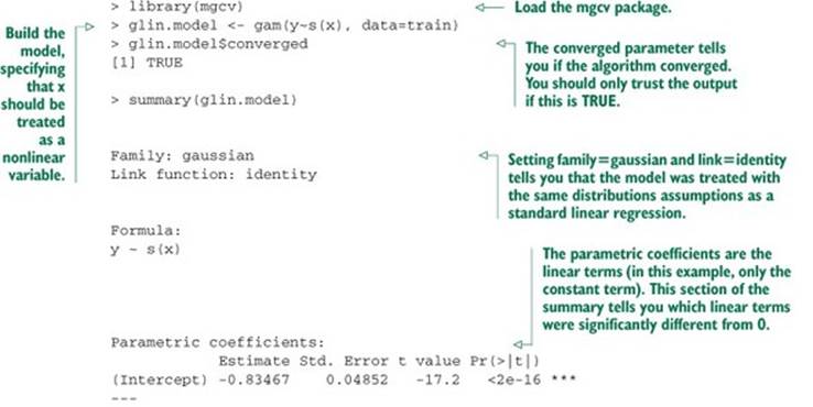
Let’s try finding a nonlinear model that maps x to y. We’ll use the function gam() in the package mgcv.^[6] When using gam(), you can model variables as either linear or nonlinear. You model a variable x as nonlinear by wrapping it in the s() notation. In this example, rather than using the formula y ~ x to describe the model, you’d use the formula y ~s(x). Then gam() will search for the spline s() that best describes the relationship between x and y, as shown in listing 9.8. Only terms surrounded by s() get the GAM/spline treatment.

⁶ There’s an older package called gam, written by Hastie and Tibshirani, the inventors of GAMs. The gam package works fine. But it’s incompatible with the mgcv package, which ggplot already loads. Since we’re using ggplot for plotting, we’ll use mgcv for our examples.

Listing 9.8. GAM applied to our artificial example

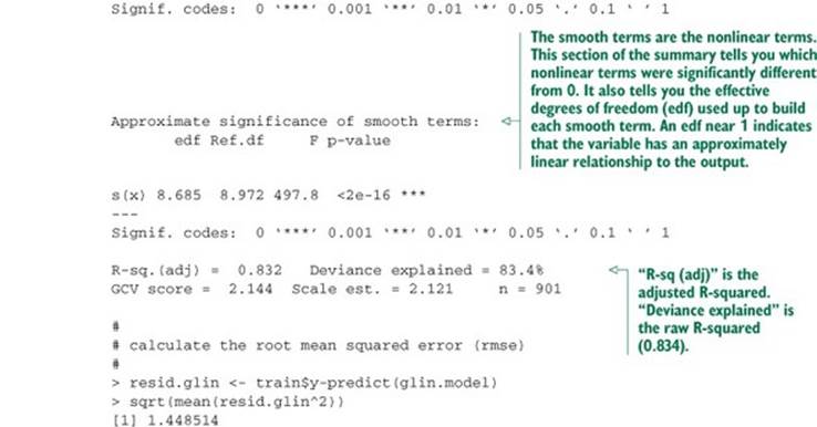
The resulting model’s predictions are plotted versus true response in figure 9.4. This fit is much better: the model explains over 80% of the variance (R-squared of 0.83), and the root mean squared error (RMSE) over the training data is less than half the RMSE of the linear model. Note that the points in figure 9.4 are distributed more or less evenly around the line of perfect prediction. The GAM has been fit to be homoscedastic, and any given prediction is as likely to be an overprediction as an underprediction.

Figure 9.4. GAM’s predictions versus actual response. The solid line is the theoretical line of perfect prediction (prediction=actual).

Modeling linear relationships using gam()

By default, gam() will perform standard linear regression. If you were to call gam() with the formula y ~ x, you’d get the same model that you got using lm(). More generally, the call gam(y ~ x1 + s(x2), data=...) would model the variable x1 as having a linear relationship withy, and try to fit the best possible smooth curve to model the relationship between x2 and y. Of course, the best smooth curve could be a straight line, so if you’re not sure whether the relationship between x and y is linear, you can use s(x). If you see that the coefficient has an edf (effective degrees of freedom—see the model summary in listing 9.8) of about 1, then you can try refitting the variable as a linear term.

The use of splines gives GAMs a richer model space to choose from; this increased flexibility brings a higher risk of overfitting. Let’s check the models’ performances on the test data.

Listing 9.9. Comparing linear regression and GAM performance

The GAM performed similarly on both sets (RMSE of 1.40 on test versus 1.45 on training; R-squared of 0.78 on test versus 0.83 on training). So there’s likely no overfit.

9.2.3. Extracting the nonlinear relationships

Once you fit a GAM, you’ll probably be interested in what the s() functions look like. Calling plot() on a GAM will give you a plot for each s() curve, so you can visualize nonlinearities. In our example, plot(glin.model) produces the top curve in figure 9.5.

Figure 9.5. Top: The nonlinear function s(PWGT) discovered by gam(), as output by plot(gam.model) Bottom: The same spline superimposed over the training data

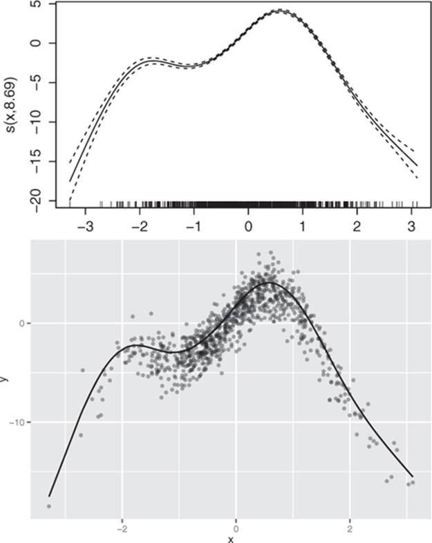
The shape of the curve is quite similar to the scatter plot we saw in figure 9.2 (which is reproduced as the lower half of figure 9.5). In fact, the spline that’s superimposed on the scatter plot in figure 9.2 is the same curve.

We can extract the data points that were used to make this graph by using the predict() function with the argument type="terms". This produces a matrix where the ith column represents s(x[,i]). Listing 9.10 demonstrates how to reproduce the lower plot in figure 9.5.

Listing 9.10. Extracting a learned spline from a GAM

> sx <- predict(glin.model, type="terms")

> summary(sx)

s(x)

Min. :-17.527035

1st Qu.: -2.378636

Median : 0.009427

Mean : 0.000000

3rd Qu.: 2.869166

Max. : 4.084999

> xframe <- cbind(train, sx=sx[,1])

> ggplot(xframe, aes(x=x)) + geom_point(aes(y=y), alpha=0.4) +

geom_line(aes(y=sx))

Now that we’ve worked through a simple example, let’s try a more realistic example with more variables.

9.2.4. Using GAM on actual data

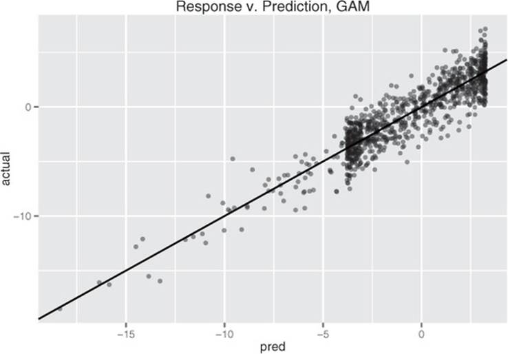
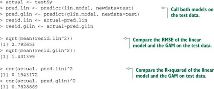
For this example, we’ll predict a newborn baby’s weight (DBWT) using data from the CDC 2010 natality dataset that we used in section 7.2 (though this is not the risk data used in that chapter).^[7] As input, we’ll consider mother’s weight (PWGT), mother’s pregnancy weight gain (WTGAIN), mother’s age (MAGER), and the number of prenatal medical visits (UPREVIS).^[8]

⁷ The dataset can be found at https://github.com/WinVector/zmPDSwR/blob/master/CDC/NatalBirthData.rData. A script for preparing the dataset from the original CDC extract can be found at https://github.com/WinVector/zmPDSwR/blob/master/CDC/prepBirthWeightData.R.

⁸ We’ve chosen this example to highlight the mechanisms of gam(), not to find the best model for birth weight. Adding other variables beyond the four we’ve chosen will improve the fit, but obscure the exposition.

In the following listing, we’ll fit a linear model and a GAM, and compare.

Listing 9.11. Applying linear regression (with and without GAM) to health data

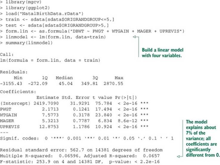
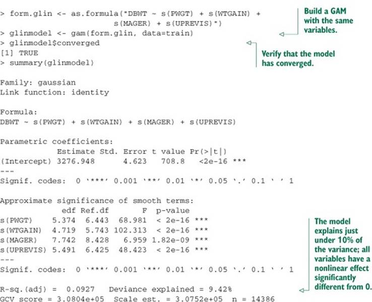
The GAM has improved the fit, and all four variables seem to have a nonlinear relationship with birth weight, as evidenced by edfs all greater than 1. We could use plot(glinmodel) to examine the shape of the s() functions; instead, we’ll compare them with a direct smoothing curve of each variable against mother’s weight.

Listing 9.12. Plotting GAM results

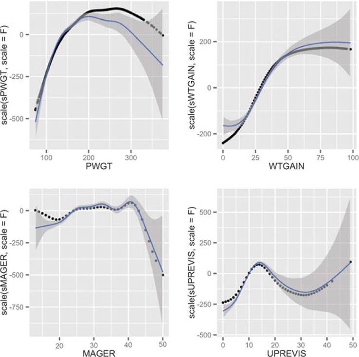
The plots of the s() splines compared with the smooth curves directly relating the input variables to birth weight are shown in figure 9.6. The smooth curves in each case are similar to the corresponding s() in shape, and nonlinear for all of the variables. As usual, we should check for overfit with hold-out data.

Figure 9.6. Smoothing curves of each of the four input variables plotted against birth weight, compared with the splines discovered by gam(). All curves have been shifted to be zero mean for comparison of shape.

Listing 9.13. Checking GAM model performance on hold-out data

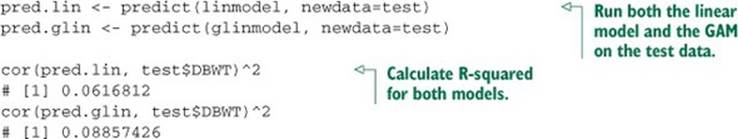
The performance of the linear model and the GAM were similar on the test set, as they were on the training set, so in this example there’s no substantial overfit.

9.2.5. Using GAM for logistic regression

The gam() function can be used for logistic regression as well. Suppose that we wanted to predict the birth of underweight babies (defined as DBWT < 2000) from the same variables we’ve been using. The logistic regression call to do that would be as shown in the following listing.

Listing 9.14. GLM logistic regression

form <- as.formula("DBWT < 2000 ~ PWGT + WTGAIN + MAGER + UPREVIS")

logmod <- glm(form, data=train, family=binomial(link="logit"))

The corresponding call to gam() also specifies the binomial family with the logit link.

Listing 9.15. GAM logistic regression

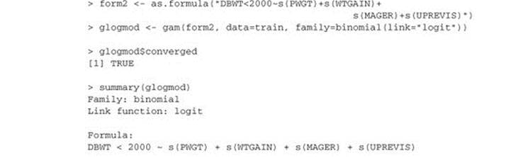
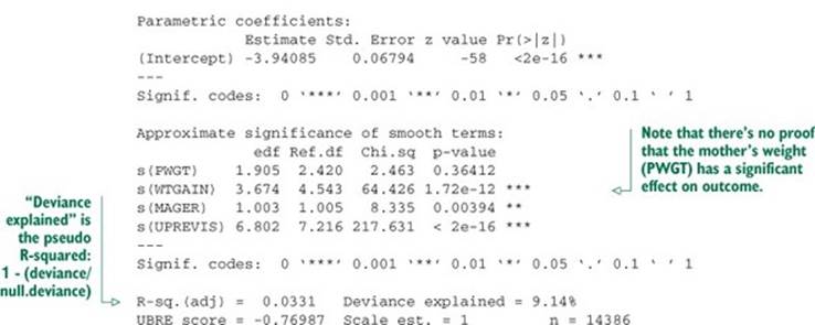
As with the standard logistic regression call, we recover the class probabilities with the call predict(glogmodel, newdata=train, type="response"). Again these models are coming out with low quality, and in practice we would look for more explanatory variables to build better screening models.

The gam() package requires explicit formulas as input

You may have noticed that when calling lm(), glm(), or rpart(), we can input the formula specification as a string. These three functions quietly convert the string into a formula object. Unfortunately, neither gam() nor randomForest(), which you saw in section 9.1.2, will do this automatic conversion. You must explicitly call as.formula() to convert the string into a formula object.

9.2.6. GAM takeaways

Here’s what you should remember about GAMs:

· GAMs let you represent nonlinear and non-monotonic relationships between variables and outcome in a linear or logistic regression framework.

· In the mgcv package, you can extract the discovered relationship from the GAM model using the predict() function with the type="terms" parameter.

· You can evaluate the GAM with the same measures you’d use for standard linear or logistic regression: residuals, deviance, R-squared, and pseudo R-squared. The gam() summary also gives you an indication of which variables have a significant effect on the model.

· Because GAMs have increased complexity compared to standard linear or logistic regression models, there’s more risk of overfit.

GAMs allow you to extend linear methods (and generalized linear methods) to allow variables to have nonlinear (or even non-monotone) effects on outcome. But we’ve only considered each variable’s impact individually. Another approach is to form new variables from nonlinear combinations of existing variables. The hope is that with access to enough of these new variables, your modeling problem becomes easier.

In the next two sections, we’ll work with two of the most popular ways to add and manage new variables: kernel methods and support vector machines.

9.3. Using kernel methods to increase data separation

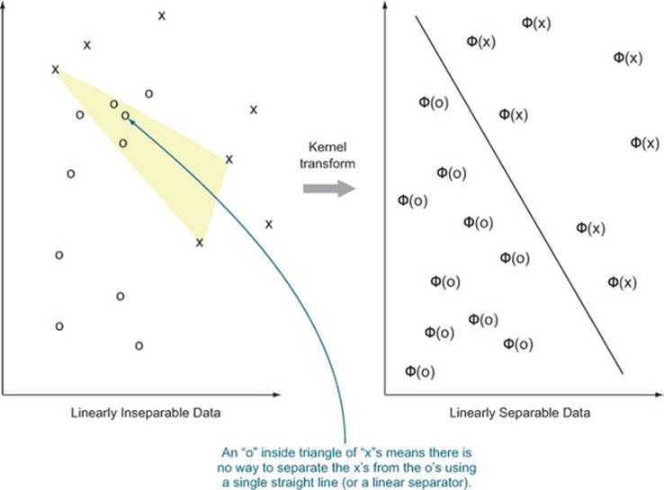
Often your available variables aren’t quite good enough to meet your modeling goals. The most powerful way to get new variables is to get new, better measurements from the domain expert. Acquiring new measurements may not be practical, so you’d also use methods to create new variables from combinations of the measurements you already have at hand. We call these new variables synthetic to emphasize that they’re synthesized from combinations of existing variables and don’t represent actual new measurements. Kernel methods are one way to produce new variables from old and to increase the power of machine learning methods.^[9] With enough synthetic variables, data where points from different classes are mixed together can often be lifted to a space where the points from each class are grouped together, and separated from out-of-class points.

⁹ The standard method to create synthetic variables is to add interaction terms. An interaction between variables occurs when a change in outcome due to two (or more) variables is more than the changes due to each variable alone. For example, too high a sodium intake will increase the risk of hypertension, but this increase is disproportionately higher for people with a genetic susceptibility to hypertension. The probability of becoming hypertensive is a function of the interaction of the two factors (diet and genetics). For details on using interaction terms in R, see help('formula'). In models such as lm(), you can introduce an interaction term by adding a colon (:) to a pair of terms in your formula specification.

One misconception about kernel methods is that they’re automatic or self-adjusting. They’re not; beyond a few “automatic bandwidth adjustments,” it’s up to the data scientist to specify a useful kernel instead of the kernel being automatically found from the data. But many of the standard kernels (inner-product, Gaussian, and cosine) are so useful that it’s often profitable to try a few kernels to see what improvements they offer.

The word kernel is used in many different senses

The word kernel has many different incompatible definitions in mathematics and statistics. The machine learning sense of the word used here is taken from operator theory and the sense used in Mercer’s theorem. The kernels we want are two argument functions that behave a lot like an inner product. The other common (incompatible) statistical use of kernel is in density estimation, where kernels are single argument functions that represent probability density functions or distributions.

In the next few sections, we’ll work through the definition of a kernel function. We’ll give a few examples of transformations that can be implemented by kernels and a few examples of transformations that can’t be implemented as kernels. We’ll then work through a few examples.

9.3.1. Understanding kernel functions

To understand kernel functions, we’ll work through the definition, why they’re useful, and some examples of important kernel functions.

Formal definition of a kernel function

In our application, a kernel is a function with a very specific definition. Let u and v be any pair of variables. u and v are typically vectors of input or independent variables (possibly taken from two rows of a dataset). A function k(,) that maps pairs (u,v) to numbers is called a kernel function if and only if there is some function phi() mapping (u,v)s to a vector space such that k(u,v) = phi(u) %*% phi(v) for all u,v.^[10] We’ll informally call the expression k(u,v) = phi(u) %*% phi(v) the Mercer expansion of the kernel (in reference to Mercer’s theorem; see http://mng.bz/xFD2) and consider phi() the certificate that tells us k(,) is a good kernel. This is much easier to understand from a concrete example. In listing 9.16, we’ll develop an example function k(,) and the matching phi() that demonstrates that k(,) is in fact a kernel over two dimensional vectors.

¹⁰ %*% is R’s notation for dot product or inner product; see help('%*%') for details. Note that phi() is allowed to map to very large (and even infinite) vector spaces.

Listing 9.16. An artificial kernel example

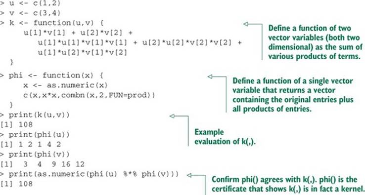
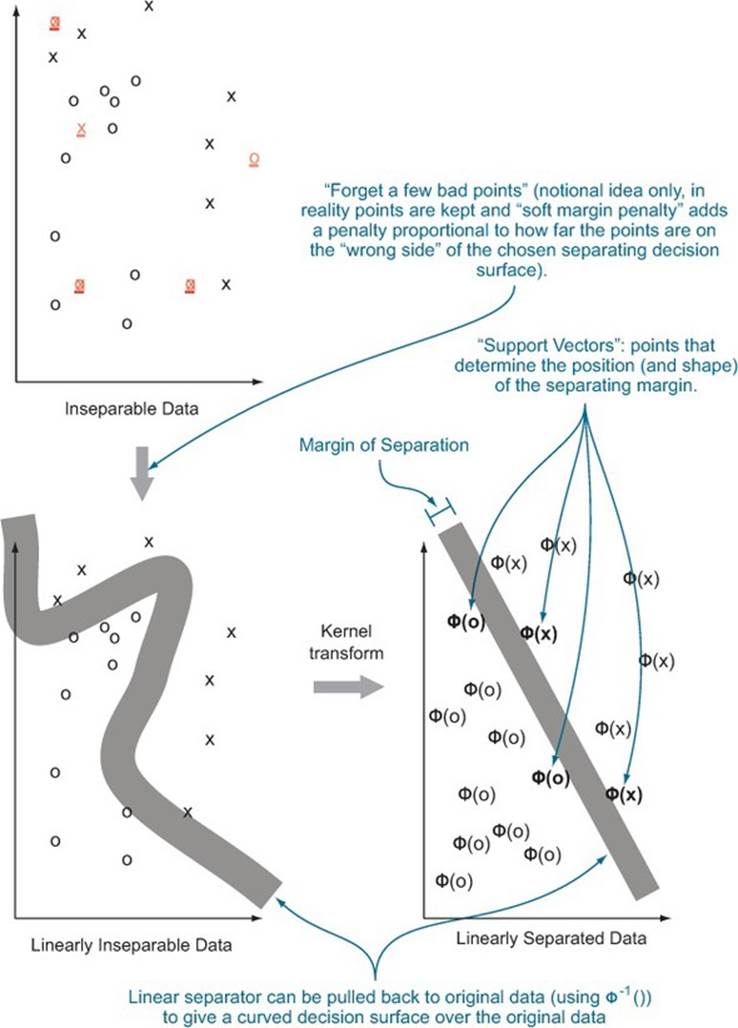
Figure 9.7 illustrates^[11] what we hope for from a good kernel: our data being pushed around so it’s easier to sort or classify. By using a kernel transformation, we move to a situation where the distinction we’re trying to learn is representable by a linear operator in our transformed data.

¹¹ See Nello Cristianini and John Shawe-Taylor, An Introduction to Support Vector Machines and Other Kernel-based Learning Methods, Cambridge University Press, 2000.

Figure 9.7. Notional illustration of a kernel transform (based on Cristianini and Shawe-Taylor, 2000)

Most kernel methods use the function k(,) directly and only use properties of k(,) guaranteed by the matching phi() to ensure method correctness. The k(,) function is usually quicker to compute than the notional function phi(). A simple example of this is what we’ll call the dot-product similarity of documents. The dot-product document similarity is defined as the dot product of two vectors where each vector is derived from a document by building a huge vector of indicators, one for each possible feature. For instance, if the features you’re considering are word pairs, then for every pair of words in a given dictionary, the document gets a feature of 1 if the pair occurs as a consecutive utterance in the document and 0 if not. This method is the phi(), but in practice we never use the phi() procedure. Instead, for one document each consecutive pair of words is generated and a bit of score is added if this pair is both in the dictionary and found consecutively in the other document. For moderatesized documents and large dictionaries, this direct k(,) implementation is vastly more efficient than the phi() implementation.

Why are kernel functions useful?

Kernel functions are useful for a number of reasons:

· Inseparable datasets (data where examples from multiple training classes appear to be intermixed when plotted) become separable (and hence we can build a good classifier) under common nonlinear transforms. This is known as Cover’s theorem. Nonlinear kernels are a good complement to many linear machine learning techniques.

· Many phi()s can be directly implemented during data preparation. Never be too proud to try some interaction variables in a model.

· Some very powerful and expensive phi()s that can’t be directly implemented during data preparation have very efficient matching kernel functions k(,) that can be used directly in select machine learning algorithms without needing access to the highly complex phi().

· All symmetric positive semidefinite functions k(,) mapping pairs of variables to the reals can be represented as k(u,v) = phi(u) %*% phi(v) for some function phi(). This is a consequence of Mercer’s theorem. So by restricting to functions with a Mercer expansion, we’re not giving up much.

Our next goal is to demonstrate some useful kernels and some machine learning algorithms that use them efficiently to solve problems. The most famous kernelized machine learning algorithm is the support vector machine, which we’ll demonstrate in section 9.4. But first it helps to demonstrate some useful kernels.

Some important kernel functions

Let’s look at some practical uses for some important kernels in table 9.1.

Table 9.1. Some important kernels and their uses

At this point, it’s important to mention that not everything is a kernel. For example, the common squared distance function (k = function(u,v) {(u-v) %*% (u-v)}) isn’t a kernel. So kernels can express similarities, but can’t directly express distances.^[12]

¹² Some more examples of kernels (and how to build new kernels from old) can be found at http://mng.bz/1F78.

Only now that we’ve touched on why some common kernels are useful is it appropriate to look at the formal mathematical definitions. Remember, we pick kernels for their utility, not because the mathematical form is exciting. Now let’s take a look at six important kernel definitions.

Mathematical definitions of common kernels

A definitional kernel is any kernel that is an explicit inner product of two applications of a vector function:

k(u, v) = Φ(u) · Φ(v)

The dot product or identity kernel is just the inner product applied to actual vectors of data:

k(u, v) = u · v

A linear transformation kernel is a matrix form like the following:

k(u, v) = u^T L^T Lv

The Gaussian or radial kernel has the following form:

k(u, v) = e ^{–c||u–v||2}

The cosine similarity kernel is a rescaled dot product kernel:

A polynomial kernel is a dot product with a transform (shift and power) applied as shown here:

k(u, v) = (su · v + c)^d

9.3.2. Using an explicit kernel on a problem

Let’s demonstrate explicitly choosing a kernel function on a problem we’ve already worked with.

Revisiting the PUMS linear regression model

To demonstrate using a kernel on an actual problem, we’ll reprepare the data used in section 7.1.3 to again build a model predicting the logarithm of income from a few other factors. We’ll resume this analysis by using load() to reload the data from a copy of the filehttps://github.com/WinVector/zmPDSwR/raw/master/PUMS/psub.RData. Recall that the basic model (for purposes of demonstration) used only a few variables; we’ll redo producing a stepwise improved linear regression model for log(PINCP).

Listing 9.17. Applying stepwise linear regression to PUMS data

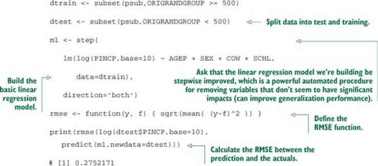
The quality of prediction was middling (the RMSE isn’t that small), but the model exposed some of the important relationships. In a real project, you’d do your utmost to find new explanatory variables. But you’d also be interested to see if any combination of variables you were already using would help with prediction. We’ll work through finding some of these combinations using an explicit phi().

Introducing an explicit transform

Explicit kernel transforms are a formal way to unify ideas like reshaping variables and adding interaction terms.^[13]

¹³ See help('formula') for how to add interactions using the : and * operators.

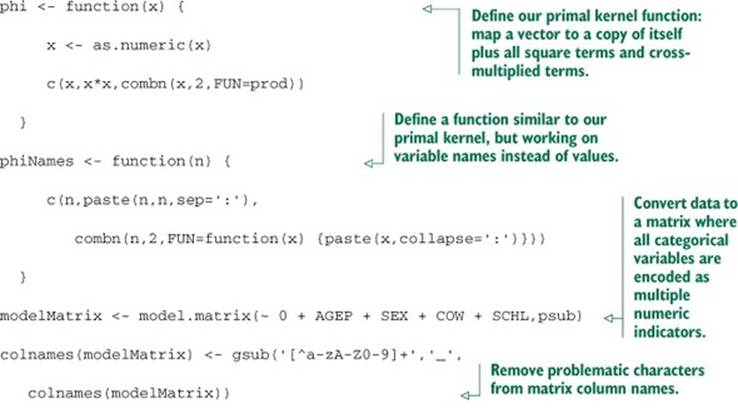
In listing 9.18, we’ll set up a phi() function and use it to build a new larger data frame with new modeling variables.

Listing 9.18. Applying an example explicit kernel transform

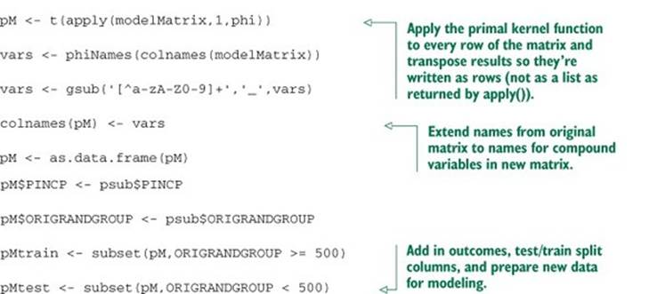
The steps to use this new expanded data frame to build a model are shown in the following listing.

Listing 9.19. Modeling using the explicit kernel transform

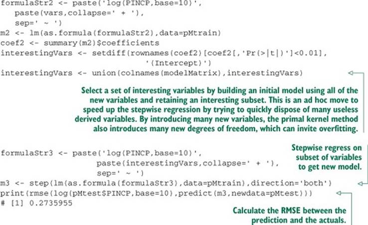
We see RMSE is improved by a small amount on the test data. With such a small improvement, we have extra reason to confirm its statistical significance using a cross-validation procedure as demonstrated in section 6.2.3. Leaving these issues aside, let’s look at the summary of the new model to see what new variables the phi() procedure introduced. The next listing shows the structure of the new model.

Listing 9.20. Inspecting the results of the explicit kernel model

> print(summary(m3))

Call:

lm(formula = log(PINCP, base = 10) ~ AGEP + SEXM +

COWPrivate_not_for_profit_employee +

SCHLAssociate_s_degree + SCHLBachelor_s_degree +

SCHLDoctorate_degree +

SCHLGED_or_alternative_credential + SCHLMaster_s_degree +

SCHLProfessional_degree + SCHLRegular_high_school_diploma +

SCHLsome_college_credit_no_degree + AGEP_AGEP, data = pMtrain)

Residuals:

Min 1Q Median 3Q Max

-1.29264 -0.14925 0.01343 0.17021 0.61968

Coefficients:

Estimate Std. Error t value Pr(>|t|)

(Intercept) 2.9400460 0.2219310 13.248 < 2e-16 ***

AGEP 0.0663537 0.0124905 5.312 1.54e-07 ***

SEXM 0.0934876 0.0224236 4.169 3.52e-05 ***

COWPrivate_not_for_profit_em -0.1187914 0.0379944 -3.127 0.00186 **

SCHLAssociate_s_degree 0.2317211 0.0509509 4.548 6.60e-06 ***

SCHLBachelor_s_degree 0.3844459 0.0417445 9.210 < 2e-16 ***

SCHLDoctorate_degree 0.3190572 0.1569356 2.033 0.04250 *

SCHLGED_or_alternative_creden 0.1405157 0.0766743 1.833 0.06737 .

SCHLMaster_s_degree 0.4553550 0.0485609 9.377 < 2e-16 ***

SCHLProfessional_degree 0.6525921 0.0845052 7.723 5.01e-14 ***

SCHLRegular_high_school_diplo 0.1016590 0.0415834 2.445 0.01479 *

SCHLsome_college_credit_no_de 0.1655906 0.0416345 3.977 7.85e-05 ***

AGEP_AGEP -0.0007547 0.0001704 -4.428 1.14e-05 ***

---

Signif. codes: 0 ’ ***’ 0.001 ’ **’ 0.01 ’ *’ 0.05 ’ .’ 0.1 ’ ’ 1

Residual standard error: 0.2649 on 582 degrees of freedom

Multiple R-squared: 0.3541, Adjusted R-squared: 0.3408

F-statistic: 26.59 on 12 and 582 DF, p-value: < 2.2e-16

In this case, the only new variable is AGEP_AGEP. The model is using AGEP*AGEP to build a non-monotone relation between age and log income.^[14]

¹⁴ Of course, this sort of relation could be handled quickly by introducing an AGEP*AGEP term directly in the model or by using a generalized additive model to discover the optimal (possibly nonlinear) shape of the relation between AGEP and log income (see section 9.2).

The phi() method is automatic and can therefore be applied in many modeling situations. In our example, we can think of the crude function that multiplies all pairs of variables as our phi() or think of the implied function that took the original set of variables to the new set calledinterestingVars as the actual training data-dependent phi(). Explicit phi() kernel notation adds some capabilities, but algorithms that are designed to work directly with implicit kernel definitions in k(,) notation can be much more powerful. The most famous such method is the support vector machine, which we’ll use in the next section.

9.3.3. Kernel takeaways

Here’s what you should remember about kernel methods:

· Kernels provide a systematic way of creating interactions and other synthetic variables that are combinations of individual variables.

· The goal of kernelizing is to lift the data into a space where the data is separable, or where linear methods can be used directly.

Now we’re ready to work with the most well-known use of kernel methods: support vector machines.

9.4. Using SVMs to model complicated decision boundaries

The idea behind SVMs is to use entire training examples as classification landmarks (called support vectors). We’ll describe the bits of the theory that affect use and move on to applications.

9.4.1. Understanding support vector machines

A support vector machine with a given function phi() builds a model where for a given example x the machine decides x is in the class if

w %*% phi(x) + b >= 0

for some w and b, and not in the class otherwise. The model is completely determined by the vector w and the scalar offset b. The general idea is sketched out in figure 9.8. In “real space” (left), the data is separated by a nonlinear boundary. When the data is lifted into the higher-dimensional kernel space (right), the lifted points are separated by a hyperplane whose normal is w and that is offset from the origin by b (not shown). Essentially, all the data that makes a positive dot product with w is on one side of the hyperplane (and all belong to one class); data that makes a negative dot product with the w belongs to the other class.

Figure 9.8. Notional illustration of SVM

Finding w and b is performed by the support vector training operation. There are variations on the support vector machine that make decisions between more than two classes, perform scoring/regression, and detect novelty. But we’ll discuss only the support vector machines for simple classification.

As a user of support vector machines, you don’t immediately need to know how the training procedure works; that’s what the software does for you. But you do need to have some notion of what it’s trying to do. The model w,b is ideally picked so that

w %*% phi(x) + b >= u

for all training xs that were in the class, and

w %*% phi(x) + b <= v

for all training examples not in the class. The data is called separable if u>v and the size of the separation (u-v)/sqrt(w %*% w) is called the margin. The goal of the SVM optimizer is to maximize the margin. A large margin can actually ensure good behavior on future data (good generalization performance). In practice, real data isn’t always separable even in the presence of a kernel. To work around this, most SVM implementations implement the so-called soft margin optimization goal.

A soft margin optimizer adds additional error terms that are used to allow a limited fraction of the training examples to be on the wrong side of the decision surface.^[15] The model doesn’t actually perform well on the altered training examples, but trades the error on these examples against increased margin on the remaining training examples. For most implementations, there’s a control that determines the trade-off between margin width for the remaining data and how much data is pushed around to achieve the margin. Typically the control is named C and setting it to values higher than 1 increases the penalty for moving data.^[16]

¹⁵ A common type of dataset that is inseparable under any kernel is any dataset where there are at least two examples belonging to different outcome classes with the exact same values for all input or x variables. The original “hard margin” SVM couldn’t deal with this sort of data and was for that reason not considered to be practical.

¹⁶ For more details on support vector machines, we recommend Cristianini and Shawe-Taylor’s An Introduction to Support Vector Machines and Other Kernel-based Learning Methods.

The support vectors

The support vector machine gets its name from how the vector w is usually represented: as a linear combination of training examples—the support vectors. Recall we said in section 9.3.1 that the function phi() is allowed, in principle, to map into a very large or even infinite vector space. Support vector machines can get away with this because they never explicitly compute phi(x). What is done instead is that any time the algorithm wants to compute phi(u) %*% phi(v) for a pair of data points, it instead computes k(u,v) which is, by definition, equal. But then how do we evaluate the final model w %*% phi(x) + b? It would be nice if there were an s such that w = phi(s), as we could then again use k(,) to do the work. In general, there’s usually no s such that w = phi(s). But there’s always a set of vectors s1,...,sm and numbers a1,...,amsuch that

w = sum(a1*phi(s1),...,am*phi(sm))

With some math, we can show this means

w %*% phi(x) + b = sum(a1*k(s1,x),...,am*k(sm,x)) + b

The right side is a quantity we can compute.

The vectors s1,...,sm are actually the features from m training examples and are called the support vectors. The work of the support vector training algorithm is to find the vectors s1,...,sm, the scalars a1,...,am, and the offset b.^[17]

¹⁷ Because SVMs work in terms of support vectors, not directly in terms of original variables or features, a feature that’s predictive can be lost if it doesn’t show up strongly in kernel-specified similarities between support vectors.

The reason why the user must know about the support vectors is because they’re stored in the support vector model and there can be a very large number of them (causing the model to be large and expensive to evaluate). In the worst case, the number of support vectors in the model can be almost as large as the number of training examples (making support vector model evaluation potentially as expensive as nearest neighbor evaluation). There are some tricks to work around this: lowering C, training models on random subsets of the training data, and primalizing.

The easy case of primalizing is when you have a kernel phi() that has a simple representation (such as the identity kernel or a low-degree polynomial kernel). In this case, you can explicitly compute a single vector w = sum(a1*phi(s1),... am*phi(sm)) and use w %*% phi(x) to classify a new x (notice you don’t need to keep the support vectors s1,...sm when you have w).

For kernels that don’t map into a finite vector space (such as the popular radial or Gaussian kernel), you can also hope to find a vector function p() such that p(u) %*% p(v) is very near k(u,v) for all of your training data and then use

w ~ sum(a1*p(s1),...,am*p(sm))

along with b as an approximation of your support vector model. But many support vector packages are unable to convert to a primal form model (it’s mostly seen in Hadoop implementations), and often converting to primal form takes as long as the original model training.

9.4.2. Trying an SVM on artificial example data

Support vector machines excel at learning concepts of the form “examples that are near each other should be given the same classification.” This is because they can use support vectors and margin to erect a moat that groups training examples into classes. In this section, we’ll quickly work some examples. One thing to notice is how little knowledge of the internal working details of the support vector machine are needed. The user mostly has to choose the kernel to control what is similar/dissimilar, adjust C to try and control model complexity, and pick class.weights to try and value different types of errors.

Spiral example

Let’s start with an example adapted from R’s kernlab library documentation. Listing 9.21 shows the recovery of the famous spiral machine learning counter-example^[18] using kernlab’s spectral clustering method.

¹⁸ See K. J. Lang and M. J. Witbrock, “Learning to tell two spirals apart,” in Proceedings of the 1988 Connectionist Models Summer School, D. Touretzky, G. Hinton, and T. Sejnowski (eds), Morgan Kaufmann, 1988 (pp. 52-59).

Listing 9.21. Setting up the spirals data as an example classification problem

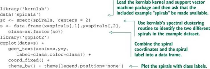
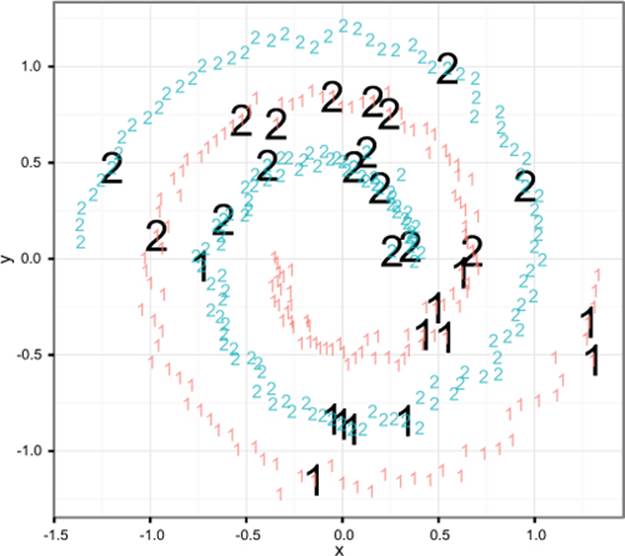
Figure 9.9 shows the labeled spiral dataset. Two classes (represented digits) of data are arranged in two interwoven spirals. This dataset is difficult for learners that don’t have a rich enough concept space (perceptrons, shallow neural nets) and easy for more sophisticated learners that can introduce the right new features. Support vector machines, with the right kernel, are a technique that finds the spiral easily.

Figure 9.9. The spiral counter-example

Support vector machines with the wrong kernel

Support vector machines are powerful, but without the correct kernel they have difficulty with some concepts (such as the spiral example). Listing 9.22 shows a failed attempt to learn the spiral concept with a support vector machine using the identity or dot-product kernel.

Listing 9.22. SVM with a poor choice of kernel

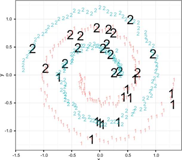
This attempt results in figure 9.10. In the figure, we plot the total dataset in light grey and the SVM classifications of the test dataset in solid black. Note that the plotted predictions look a lot more like the concept y < 0 than the spirals. The SVM didn’t produce a good model with the identity kernel. In the next section, we’ll repeat the process with the Gaussian radial kernel and get a much better result.

Figure 9.10. Identity kernel failing to learn the spiral concept

Support vector machines with a good kernel

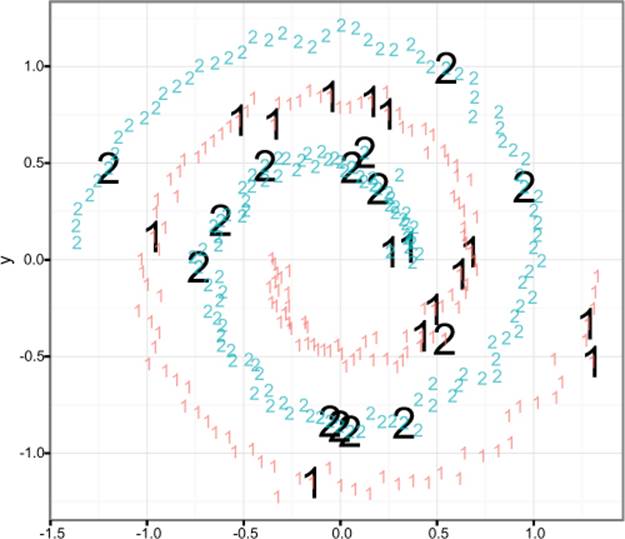
In listing 9.23, we’ll repeat the SVM fitting process, but this time specifying the Gaussian or radial kernel. We’ll again plot the SVM test classifications in black (with the entire dataset in light grey) in figure 9.11. Note that this time the actual spiral has been learned and predicted.

Figure 9.11. Radial kernel successfully learning the spiral concept

Listing 9.23. SVM with a good choice of kernel

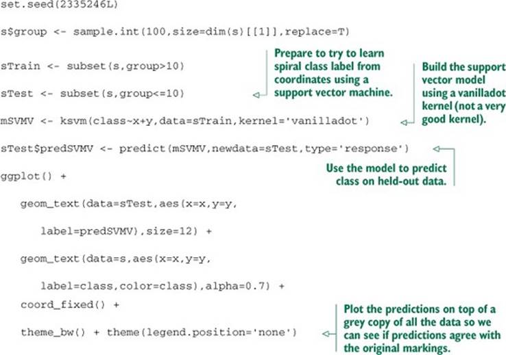
9.4.3. Using SVMs on real data

To demonstrate the use of SVMs on real data, we’ll quickly redo the analysis of the Spambase data from section 5.2.1.

Repeating the Spambase logistic regression analysis

In section 5.2.1, we originally built a logistic regression model and confusion matrix. We’ll continue working on this example in listing 9.24 (after downloading the dataset from https://github.com/WinVector/zmPDSwR/raw/master/Spambase/spamD.tsv).

Listing 9.24. Revisiting the Spambase example with GLM

spamD <- read.table('spamD.tsv',header=T,sep='\t')

spamTrain <- subset(spamD,spamD$rgroup>=10)

spamTest <- subset(spamD,spamD$rgroup<10)

spamVars <- setdiff(colnames(spamD),list('rgroup','spam'))

spamFormula <- as.formula(paste('spam=="spam"',

paste(spamVars,collapse=' + '),sep=' ~ '))

spamModel <- glm(spamFormula,family=binomial(link='logit'),

data=spamTrain)

spamTest$pred <- predict(spamModel,newdata=spamTest,

type='response')

print(with(spamTest,table(y=spam,glPred=pred>=0.5)))

## glPred

## y FALSE TRUE

## non-spam 264 14

## spam 22 158

Applying a support vector machine to the Spambase example

The SVM modeling steps are about as simple as the previous regression analysis, and are shown in the following listing.

Listing 9.25. Applying an SVM to the Spambase example

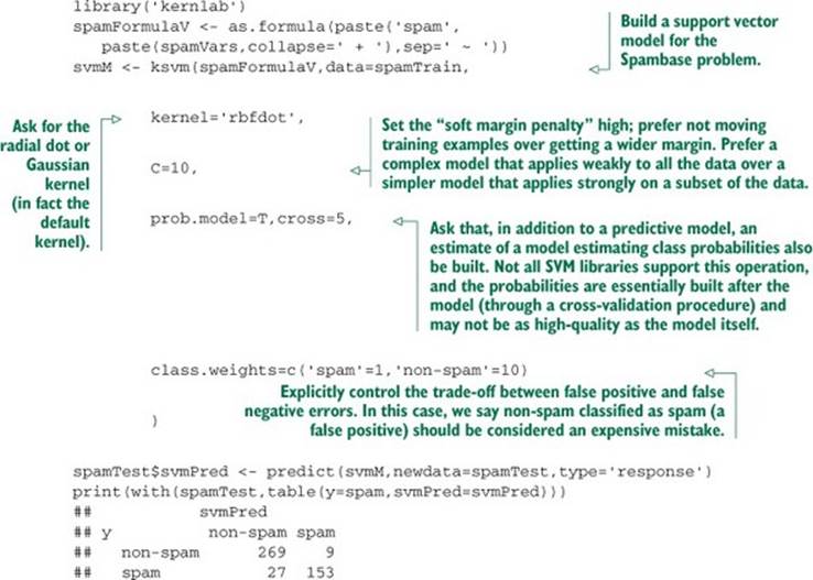
Listing 9.26 shows the standard summary and print display for the support vector model. Very few model diagnostics are included (other than training error, which is a simple accuracy measure), so we definitely recommend using the model critique techniques from chapter 5 to validate model quality and utility. A few things to look for are which kernel was used, the SV type (classification is the type we want),^[19] and the number of support vectors retained (this is the degree of memorization going on). In this case, 1,118 training examples were retained as support vectors, which seems like way too complicated a model, as this number is much larger than the original number of variables (57) and with an order of magnitude of the number of training examples (4143). In this case, we’re seeing more memorization than useful generalization.

¹⁹ The ksvm call only performs classification on factors; if a Boolean or numeric quantity is used as the quantity to be predicted, the ksvm call may return a regression model (instead of the desired classification model).

Listing 9.26. Printing the SVM results summary

print(svmM)

Support Vector Machine object of class "ksvm"

SV type: C-svc (classification)

parameter : cost C = 10

Gaussian Radial Basis kernel function.

Hyperparameter : sigma = 0.0299836801848002

Number of Support Vectors : 1118

Objective Function Value : -4642.236

Training error : 0.028482

Cross validation error : 0.076998

Probability model included.

Comparing results

Note that the two confusion matrices are very similar. But the SVM model has a lower false positive count of 9 than the GLM’s 14. Some of this is due to setting C=10 (which tells the SVM to prefer training accuracy and margin over model simplicity) and setting class.weights (telling the SVM to prefer precision over recall). For a more apples-to-apples comparison, we can look at the GLM model’s top 162 spam candidates (the same number the SVM model proposed: 153 + 9).

Listing 9.27. Shifting decision point to perform an apples-to-apples comparison

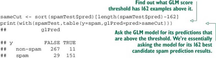
Note that the new shifted GLM confusion matrix in listing 9.27 is pretty much indistinguishable from the SVM confusion matrix. Where SVMs excel is in cases where unknown combinations of variables are important effects, and also when similarity of examples is strong evidence of examples being in the same class (not a property of the email spam example we have here). Problems of this nature tend to benefit from use of either SVM or nearest neighbor techniques.^[20]

²⁰ For some examples of the connections between support vector machines and kernelized nearest neighbor methods please see http://mng.bz/1F78.

9.4.4. Support vector machine takeaways

Here’s what you should remember about SVMs:

· SVMs are a kernel-based classification approach where the kernels are represented in terms of a (possibly very large) subset of the training examples.

· SVMs try to lift the problem into a space where the data is linearly separable (or as near to separable as possible).

· SVMs are useful in cases where the useful interactions or other combinations of input variables aren’t known in advance. They’re also useful when similarity is strong evidence of belonging to the same class.

9.5. Summary

In this chapter, we demonstrated some advanced methods to fix specific issues with basic modeling approaches. We used

· Bagging and random forests— To reduce the sensitivity of models to early modeling choices and reduce modeling variance

· Generalized additive models— To remove the (false) assumption that each model feature contributes to the model in a monotone fashion

· Kernel methods— To introduce new features that are nonlinear combinations of existing features, increasing the power of our model

· Support vector machines— To use training examples as landmarks (support vectors), again increasing the power of our model

You should understand that you bring in advanced methods and techniques to fix specific modeling problems, not because they have exotic names or exciting histories. We also feel you should at least try to find an existing technique to fix a problem you suspect is hiding in your data beforebuilding your own custom technique (often the existing technique incorporates a lot of tuning and wisdom). Finally, the goal of learning the theory of advanced techniques is not to be able to recite the steps of the common implementations, but to know when the techniques apply and what trade-offs they represent. The data scientist needs to supply thought and judgment and realize that the platform can supply implementations.

The actual point of a modeling project is to deliver results for deployment and to present useful documentation and evaluations to your partners. The next part of this book will address best practices for delivering your results.

Key takeaways

· Use advanced methods to fix specific problems, not for the excitement.

· Advanced methods can help fix overfit, variable interactions, non-additive relations, and unbalanced distributions, but not lack of features or data.

· Which method is best depends on the data, and there are many advanced methods to try.

· Only deliver advanced models if you can show they are outperforming simpler methods.