From Mathematics to Generic Programming (2011)

2. The First Algorithm

Moses speedily learned arithmetic, and geometry.
...This knowledge he derived from the Egyptians,
who study mathematics above all things.
Philo of Alexandria, Life of Moses

An algorithm is a terminating sequence of steps for accomplishing a computational task. Algorithms are so closely associated with the notion of computer programming that most people who know the term probably assume that the idea of algorithms comes from computer science. But algorithms have been around for literally thousands of years. Mathematics is full of algorithms, some of which we use every day. Even the method schoolchildren learn for long addition is an algorithm.

Despite its long history, the notion of an algorithm didn’t always exist; it had to be invented. While we don’t know when algorithms were first invented, we do know that some algorithms existed in Egypt at least as far back as 4000 years ago.

* * *

Ancient Egyptian civilization was centered on the Nile River, and its agriculture depended on the river’s floods to enrich the soil. The problem was that every time the Nile flooded, all the markers showing the boundaries of property were washed away. The Egyptians used ropes to measure distances, and developed procedures so they could go back to their written records and reconstruct the property boundaries. A select group of priests who had studied these mathematical techniques were responsible for this task; they became known as “rope-stretchers.” The Greeks would later call them geometers, meaning “Earth-measurers.”

Unfortunately, we have little written record of the Egyptians’ mathematical knowledge. Only two mathematical documents survived from this period. The one we are concerned with is called the Rhind Mathematical Papyrus, named after the 19th-century Scottish collector who bought it in Egypt. It is a document from about 1650 BC written by a scribe named Ahmes, which contains a series of arithmetic and geometry problems, together with some tables for computation. This scroll contains the first recorded algorithm, a technique for fast multiplication, along with a second one for fast division. Let’s begin by looking at the fast multiplication algorithm, which (as we shall see later in the book) is still an important computational technique today.

2.1 Egyptian Multiplication

The Egyptians’ number system, like that of all ancient civilizations, did not use positional notation and had no way to represent zero. As a result, multiplication was extremely difficult, and only a few trained experts knew how to do it. (Imagine doing multiplication on large numbers if you could only manipulate something like Roman numerals.)

How do we define multiplication? Informally, it’s “adding something to itself a number of times.” Formally, we can define multiplication by breaking it into two cases: multiplying by 1, and multiplying by a number larger than 1.

We define multiplication by 1 like this:

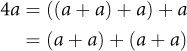
Next we have the case where we want to compute a product of one more thing than we already computed. Some readers may recognize this as the process of induction; we’ll use that technique more formally later on.

One way to multiply n by a is to add instances of a together n times. However, this could be extremely tedious for large numbers, since n – 1 additions are required. In C++, the algorithm looks like this:

Click here to view code image

int multiply0(int n, int a) {
if (n == 1) return a;
return multiply0(n - 1, a) + a;
}

The two lines of code correspond to equations 2.1 and 2.2. Both a and n must be positive, as they were for the ancient Egyptians.

The algorithm described by Ahmes—which the ancient Greeks knew as “Egyptian multiplication” and which many modern authors refer to as the “Russian Peasant Algorithm”¹—relies on the following insight:

¹ Many computer scientists learned this name from Knuth’s The Art of Computer Programming, which says that travelers in 19th-century Russia observed peasants using the algorithm. However, the first reference to this story comes from a 1911 book by Sir Thomas Heath, which actually says, “I have been told that there is a method in use today (some say in Russia, but I have not been able to verify this), ....”

This optimization depends on the law of associativity of addition:

a + (b + c) = (a + b) + c

It allows us to compute a + a only once and reduce the number of additions.

The idea is to keep halving n and doubling a, constructing a sum of power-of-2 multiples. At the time, algorithms were not described in terms of variables such as a and n; instead, the author would give an example and then say, “Now do the same thing for other numbers.” Ahmes was no exception; he demonstrated the algorithm by showing the following table for multiplying n = 41 by a = 59:

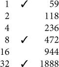
Each entry on the left is a power of 2; each entry on the right is the result of doubling the previous entry (since adding something to itself is relatively easy). The checked values correspond to the 1-bits in the binary representation of 41. The table basically says that

41 × 59 = (1 × 59) + (8 × 59) + (32 × 59)

where each of the products on the right can be computed by doubling 59 the correct number of times.

The algorithm needs to check whether n is even and odd, so we can infer that the Egyptians knew of this distinction, although we do not have direct proof. But ancient Greeks, who claimed that they learned their mathematics from the Egyptians, certainly did. Here’s how they defined² even and odd, expressed in modern notation:³

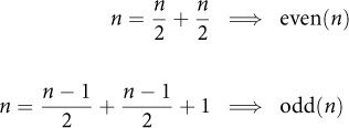
² The definition appears in the 1st-century work Introduction to Arithmetic, Book I, Chapter VII, by Nicomachus of Gerasa. He writes, “The even is that which can be divided into two equal parts without a unit intervening in the middle; and the odd is that which cannot be divided into two equal parts because of the aforesaid intervention of a unit.”

³ The arrow symbol “” is read “implies.” See Appendix A for a summary of the mathematical notation used in this book.

We will also rely on this requirement:

odd(n) half(n) = half(n – 1)

This is how we express the Egyptian multiplication algorithm in C++:

Click here to view code image

int multiply1(int n, int a) {
if (n == 1) return a;
int result = multiply1(half(n), a + a);
if (odd(n)) result = result + a;
return result;
}

We can easily implement odd(x) by testing the least significant bit of x, and half(x) by a single right shift of x:

Click here to view code image

bool odd(int n) { return n & 0x1; }
int half(int n) { return n >> 1; }

How many additions is multiply1 going to do? Every time we call the function, we’ll need to do the addition indicated by the + in a + a. Since we are halving the value as we recurse, we’ll invoke the function log n times.⁴And some of the time, we’ll need to do another addition indicated by the + in result + a. So the total number of additions will be

#₊(n) = log n + (ν(n) – 1)

⁴ Throughout this book, when we write “log,” we mean the base 2 logarithm, unless specified otherwise.

where v(n) is the number of 1s in the binary representation of n (the population count or pop count). So we have reduced an O(n) algorithm to one that is O(log n).

Is this algorithm optimal? Not always. For example, if we want to multiply by 15, the preceding formula would give this result:

#₊(15) = 3 + 4 – 1 = 6

But we can actually multiply by 15 with only 5 additions, using the following procedure:

Click here to view code image

int multiply_by_15(int a) {
int b = (a + a) + a; // b == 3*a
int c = b + b; // c == 6*a
return (c + c) + b; // 12*a + 3*a
}

Such a sequence of additions is called an addition chain. Here we have discovered an optimal addition chain for 15. Nevertheless, Ahmes’s algorithm is good enough for most purposes.

Exercise 2.1. Find optimal addition chains for n < 100.

At some point the reader may have observed that some of these computations would be even faster if we first reversed the order of the arguments when the first is greater than the second (for example, we could compute 3 × 15 more easily than 15 × 3). That’s true, and the Egyptians knew this. But we’re not going to add that optimization here, because as we’ll see in Chapter 7, we’re eventually going to want to generalize our algorithm to cases where the arguments have different types and the order of the arguments matters.

2.2 Improving the Algorithm

Our multiply1 function works well as far as the number of additions is concerned, but it also does log n recursive calls. Since function calls are expensive, we want to transform the program to avoid this expense.

One principle we’re going to take advantage of is this: It is often easier to do more work rather than less. Specifically, we’re going to compute

r + na

where r is a running result that accumulates the partial products na. In other words, we’re going to perform multiply-accumulate rather than just multiply. This principle turns out to be true not only in programming but also in hardware design and in mathematics, where it’s often easier to prove a general result than a specific one.

Here’s our multiply-accumulate function:

Click here to view code image

int mult_acc0(int r, int n, int a) {
if (n == 1) return r + a;
if (odd(n)) {
return mult_acc0(r + a, half(n), a + a);
} else {
return mult_acc0(r, half(n), a + a);
}
}

It obeys the invariant: r + na = r₀ + n₀a₀, where r₀, n₀ and a₀ are the initial values of those variables.

We can improve this further by simplifying the recursion. Notice that the two recursive calls differ only in their first argument. Instead of having two recursive calls for the odd and even cases, we’ll just modify the value of r before we recurse, like this:

Click here to view code image

int mult_acc1(int r, int n, int a) {
if (n == 1) return r + a;
if (odd(n)) r = r + a;
return mult_acc1(r, half(n), a + a);
}

Now our function is tail-recursive—that is, the recursion occurs only in the return value. We’ll take advantage of this fact shortly.

We make two observations:

• n is rarely 1.

• If n is even, there’s no point checking to see if it’s 1.

So we can reduce the number of times we have to compare with 1 by a factor of 2, simply by checking for oddness first:

Click here to view code image

int mult_acc2(int r, int n, int a) {
if (odd(n)) {
r = r + a;
if (n == 1) return r;
}
return mult_acc2(r, half(n), a + a);
}

Some programmers think that compiler optimizations will do these kinds of transformations for us, but that’s rarely true; they do not transform one algorithm into another.

What we have so far is pretty good, but we’re eventually going to want to eliminate the recursion to avoid the function call overhead. This is easier if the function is strictly tail-recursive.

Definition 2.1. A strictly tail-recursive procedure is one in which all the tail-recursive calls are done with the formal parameters of the procedure being the corresponding arguments.

Again, we can achieve this simply by assigning the desired values to the variables we’ll be passing before we do the recursion:

Click here to view code image

int mult_acc3(int r, int n, int a) {
if (odd(n)) {
r = r + a;
if (n == 1) return r;
}
n = half(n);
a = a + a;
return mult_acc3(r, n, a);
}

Now it is easy to convert this to an iterative program by replacing the tail recursion with a while(true) construct:

Click here to view code image

int mult_acc4(int r, int n, int a) {
while (true) {
if (odd(n)) {
r = r + a;
if (n == 1) return r;
}
n = half(n);
a = a + a;
}
}

With our newly optimized multiply-accumulate function, we can write a new version of multiply. Our new version will invoke our multiply-accumulate helper function:

Click here to view code image

int multiply2(int n, int a) {
if (n == 1) return a;
return mult_acc4(a, n - 1, a);
}

Notice that we skip one iteration of mult_acc4 by calling it with result already set to a.

This is pretty good, except when n is a power of 2. The first thing we do is subtract 1, which means that mult_acc4 will be called with a number whose binary representation is all 1s, the worst case for our algorithm. So we’ll avoid this by doing some of the work in advance when n is even, halving it (and doubling a) until n becomes odd:

Click here to view code image

int multiply3(int n, int a) {
while (!odd(n)) {
a = a + a;
n = half(n);
}
if (n == 1) return a;
return mult_acc4(a, n - 1, a);
}

But now we notice that we’re making mult_acc4 do one unnecessary test for n = 1, because we’re calling it with an even number. So we’ll do one halving and doubling on the arguments before we call it, giving us our final version:

Click here to view code image

int multiply4(int n, int a) {
while (!odd(n)) {
a = a + a;
n = half(n);
}
if (n == 1) return a;
// even(n – 1) n – 1 ≠ 1
return mult_acc4(a, half(n - 1), a + a);
}