From Mathematics to Generic Programming (2011)
3. Ancient Greek Number Theory
Pythagoreans applied themselves to the study of mathematics....
They thought that its principles must be the principles of all existing things.
Aristotle, Metaphysics
In this chapter, we’re going to look at some of the problems studied by ancient Greek mathematicians. Their work on patterns and “shapes” of numbers led to the discovery of prime numbers and the beginnings of a field of mathematics called number theory. They also discovered paradoxes that ultimately produced some mathematical breakthroughs. Along the way, we’ll examine an ancient algorithm for finding primes, and see how to optimize it.
3.1 Geometric Properties of Integers
Pythagoras, the Greek mathematician and philosopher who most of us know only for his theorem, was actually the person who came up with the idea that understanding mathematics is necessary to understand the world. He also discovered many interesting properties of numbers; he considered this understanding to be of great value in its own right, independent of any practical application. According to Aristotle’s pupil Aristoxenus, “He attached supreme importance to the study of arithmetic, which he advanced and took out of the region of commercial utility.”
Pythagoras (ca. 570 BC–ca. 490 BC)
Pythagoras was born on the Greek island of Samos, which was a major naval power at the time. He came from a prominent family, but chose to pursue wisdom rather than wealth. At some point in his youth he traveled to Miletus to study with Thales, the founder of philosophy (see Section 9.2), who advised him to go to Egypt and learn the Egyptians’ mathematical secrets.
During the time Pythagoras was studying abroad, the Persian empire conquered Egypt. Pythagoras followed the Persian army eastward to Babylon (in what is now Iraq), where he learned Babylonian mathematics and astronomy. While there, he may have met travelers from India; what we know is that he was exposed to and began espousing ideas we typically associate with Indian religions, including the transmigration of souls, vegetarianism, and asceticism. Prior to Pythagoras, these ideas were completely unknown to the Greeks.
After returning to Greece, Pythagoras started a settlement in Croton, a Greek colony in southern Italy, where he gathered followers—both men and women—who shared his ideas and followed his ascetic lifestyle. Their lives were centered on the study of four things: astronomy, geometry, number theory, and music. These four subjects, later known as the quadrivium, remained a focus of European education for 2000 years. Each of these disciplines was related: the motion of the stars could be mapped geometrically, geometry could be grounded in numbers, and numbers generated music. In fact, Pythagoras was the first to discover the numerical structure of frequencies in musical octaves. His followers said that he could “hear the music of the celestial spheres.”
After the death of Pythagoras, the Pythagoreans spread to several other Greek colonies in the area and developed a large body of mathematics. However, they kept their teachings secret, so many of their results may have been lost. They also eliminated competition within their ranks by crediting all discoveries to Pythagoras himself, so we don’t actually know which individuals did what.
Although the Pythagorean communities were gone after a couple of hundred years, their work remains influential. As late as the 17th century, Leibniz (one of the inventors of calculus) described himself as a Pythagorean.
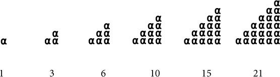
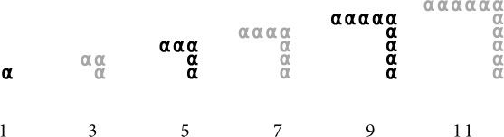
Unfortunately, Pythagoras and his followers kept their work secret, so none of their writings survive. However, we know from contemporaries what some of his discoveries were. Some of these come from a first-century book called Introduction to Arithmetic by Nicomachus of Gerasa. These included observations about geometric properties of numbers; they associated numbers with particular shapes.
Triangular numbers, for example, which are formed by stacking rows representing the first n integers, are those that formed the following geometric pattern:
Oblong numbers are those that look like this:
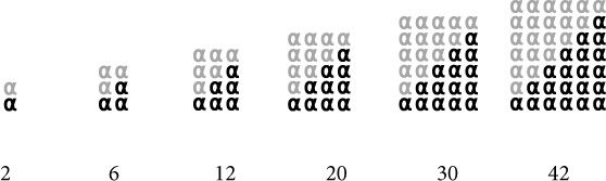
It is easy to see that the nth oblong number is represented by an n × (n + 1) rectangle:
![]() n = n(n + 1)
n = n(n + 1)
It’s also clear geometrically that each oblong number is twice its corresponding triangular number. Since we already know that triangular numbers are the sum of the first n integers, we have
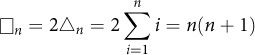
So the geometric representation gives us the formula for the sum of the first n integers:
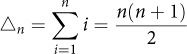
Another geometric observation is that the sequence of odd numbers forms the shape of what the Greeks called gnomons (the Greek word for a carpenter’s square; a gnomon is also the part of a sundial that casts the shadow):
Combining the first n gnomons creates a familiar shape—a square:
This picture also gives us a formula for the sum of the first n odd numbers:
Exercise 3.1. Find a geometric proof for the following: take any triangular number, multiply it by 8, and add 1. The result is a square number. (This problem comes from Plutarch’s Platonic Questions.)
3.2 Sifting Primes
Pythagoreans also observed that some numbers could not be made into any nontrivial rectangular shape (a shape where both sides of the rectangle are greater than 1). These are what we now call prime numbers—numbers that are not products of smaller numbers:
2, 3, 5, 7, 11, 13,...
(“Numbers” for the Greeks were always whole numbers.) Some of the earliest observations about primes come from Euclid. While he is usually associated with geometry, several books of Euclid’s Elements actually discuss what we now call number theory. One of his results is this theorem:
Theorem 3.1 (Euclid VII, 32): Any number is either prime or divisible by some prime.
The proof, which uses a technique called “impossibility of infinite descent,” goes like this:1
1 Euclid’s proof of VII, 32 actually relies on his proposition VII, 31 (any composite number is divisible by some prime), which contains the reasoning shown here.
Proof. Consider a number A. If it is prime, then we are done. If it is composite (i.e., nonprime), then it must be divisible by some smaller number B. If B is prime, we are done (because if A is divisible by B and B is prime, then A is divisible by a prime). If B is composite, then it must be divisible by some smaller number C, and so on. Eventually, we will find a prime or, as Euclid remarks in his proof of the previous proposition, “an infinite sequence of numbers will divide the number, each of which is less than the other; and this is impossible.”
![]()
This Euclidean principle that any descending sequence of natural numbers terminates is equivalent to the induction axiom of natural numbers, which we will encounter in Chapter 9.
* * *
Another result, which some consider the most beautiful theorem in mathematics, is the fact that there are infinitely many primes:
Theorem 3.2 (Euclid IX, 20): For any sequence of primes {p1,...,pn}, there is a prime p not in the sequence.
Proof. Consider the number
where pi is the ith prime in the sequence. Because of the way we constructed q, we know it is not divisible by any pi. Then either q is prime, in which case it is itself a prime not in the sequence, or q is divisible by some new prime, which by definition is not in the sequence. Therefore, there are infinitely many primes.
![]()
One of the best-known techniques for finding primes is the Sieve of Eratosthenes. Eratosthenes was a 3rd-century Greek mathematician who is remembered in part for his amazingly accurate measurement of the circumference of the Earth. Metaphorically, the idea of Eratosthenes’ sieve is to “sift” all the numbers so that the nonprimes “fall through” the sieve and the primes remain at the end. The actual procedure is to start with a list of all the candidate numbers and then cross out the ones known not to be primes (since they are multiples of primes found so far); whatever is left are the primes. Today the Sieve of Eratosthenes is often shown starting with all positive integers up to a given number, but Eratosthenes already knew that even numbers were not prime, so he didn’t bother to include them.
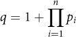
Following Eratosthenes’ convention, we’ll also include only odd numbers, so our sieve will find primes greater than 2. Each value in the sieve is a candidate prime up to whatever value we care about. If we want to find primes up to a maximum of m = 53, our sieve initially looks like this:
![]()
In each iteration, we take the first number (which must be a prime) and cross out all the multiples except itself that have not previously been crossed out. We’ll highlight the numbers being crossed out in the current iteration by boxing them. Here’s what the sieve looks like after we cross out the multiples of 3:
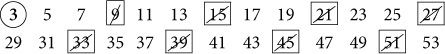
Next we cross out the multiples of 5 that have not yet been crossed out:
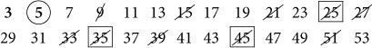
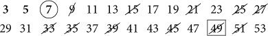
And then the remaining multiples of 7:
We need to repeat this process until we’ve crossed out all the multiples of factors less than or equal to ![]() , where m is the highest candidate we’re considering.
, where m is the highest candidate we’re considering.
In our example, m = 53, so we are done. All the numbers that have not been crossed out are primes:
![]()
Before we write our implementation of the algorithm, we’ll make a few observations. Let’s go back to what the sieve looked like in the middle of the process (say, when we were crossing out multiples of 5) and add some information—namely, the index, or position in the list, of each candidate being considered:
![]()
Notice that when we’re considering multiples of factor 5, the step size—the number of entries between two numbers being crossed out, such as 25 and 35—is 5, the same as the factor. Another way to say this is that the difference between the indexes of any two candidates being crossed out in a given iteration is the same as the factor being used. Also, since the list of candidates contains only odd numbers, the difference between two values is twice as much as the difference between two indexes. So the difference between two numbers being crossed out in a given iteration (e.g., between 25 and 35) is twice the step size or, equivalently, twice the factor being used. You’ll see that this pattern holds for all the factors we considered in our example as well.
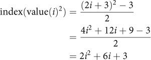
Finally, we observe that the first number crossed out in each iteration is the square of the prime factor being used. That is, when we’re crossing out multiples of 5, the first one that wasn’t previously crossed out is 25. This is because all the other multiples were already accounted for by previous primes.
3.3 Implementing and Optimizing the Code
At first glance it seems like our algorithm will need to maintain two arrays: one containing the candidate numbers we’re sifting—the “values”—and another containing Boolean flags indicating whether the corresponding number is still there or has been crossed out. However, after a bit of thought it becomes clear that we don’t actually need to store the values at all. Most of the values (namely, all the nonprimes) are never used. When we do need a value, we can compute it from its position; we know that the first value is 3 and that each successive value is 2 more than the previous one, so the ith value is 2i + 3.
So our implementation will store just the Boolean flags in the sieve, using true for prime and false for composite. We call the process of “crossing out” nonprimes marking the sieve. Here’s a function we’ll use to mark all the nonprimes for a given factor:
Click here to view code image
template <RandomAccessIterator I, Integer N>
void mark_sieve(I first, I last, N factor) {
// assert(first != last)
*first = false;
while (last - first > factor) {
first = first + factor;
*first = false;
}
}
We are using the convention of “declaring” our template arguments with a description of their requirements. We will discuss these requirements, known as concepts, in detail later on in Chapter 10; for now, readers can consult Appendix C as a reference. (If you are not familiar with C++ templates, these are also explained in this appendix.)
As we’ll see shortly, we’ll call this function with first pointing to the Boolean value corresponding to the first “uncrossed-out” multiple of factor, which as we saw is always factor’s square. For last, we’ll follow the STL convention of passing an iterator that points just past the last element in our table, so that last - first is the number of elements.
* * *
Before we see how to sift, we observe the following sifting lemmas:
• The square of the smallest prime factor of a composite number c is less than or equal to c.
• Any composite number less than p2 is sifted by (i.e., crossed out as a multiple of) a prime less than p.
• When sifting by p, start marking at p2.
• If we want to sift numbers up to m, stop sifting when p2 > m.
We will use the following formulas in our computation:
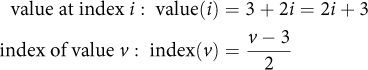
step between multiple k and multiple k + 1 of value at i:
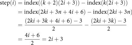
index of square of value at i:
We can now make our first attempt at implementing the sieve:
Click here to view code image
template <RandomAccessIterator I, Integer N>
void sift0(I first, N n) {
std::fill(first, first + n, true);
N i(0);
N index_square(3);
while (index_square < n) {
// invariant: index_square = 2i^2 + 6i + 3
if (first[i]) { // if candidate is prime
mark_sieve(first + index_square,
first + n, // last
i + i + 3); // factor
}
++i;
index_square = 2*i*(i + 3) + 3;
}
}
It might seem that we should pass in a reference to a data structure containing the Boolean sequence, since the sieve works only if we sift the whole thing. But by instead passing an iterator to the beginning of the range, together with its length, we don’t constrain which kind of data structure to use. The data could be in an STL container or in a block of memory; we don’t need to know. Note that we use the size of the table n rather than the maximum value to sift m.
The variable index_square is the index of the first value we want to mark—that is, the square of the current factor. One thing we notice is that we’re computing the factor we use to mark the sieve (i + i + 3) and other quantities (shown in slanted text) every time through the loop. We can hoist common subexpressions out of the loop; the changes are shown in bold:
Click here to view code image
template <RandomAccessIterator I, Integer N>
void sift1(I first, N n) {
I last = first + n;
std::fill(first, last, true);
N i(0);
N index_square(3);
N factor(3);
while (index_square < n) {
// invariant: index_square = 2i^2 + 6i + 3,
// factor = 2i + 3
if (first[i]) {
mark_sieve(first + index_square, last, factor);
}
++i;
factor = i + i + 3;
index_square = 2*i*(i + 3) + 3;
}
}
The astute reader will notice that the factor computation is actually slightly worse than before, since it happens every time through the loop, not just on iterations when the if test is true. However, we shall see later why making factor a separate variable makes sense. A bigger issue is that we still have a relatively expensive operation—the computation of index_square, which involves two multiplications. So we will take a cue from compiler optimization and use a technique known as strength reduction, which was designed to replace more expensive operations like multiplication with equivalent code that uses less expensive operations like addition.2 If a compiler can do this automatically, we can certainly do it manually.
2 While multiplication is not necessarily slower than addition on modern processors, the general technique can still lead to using fewer operations.
Let’s look at these computations in more detail. Suppose we replaced
Click here to view code image
factor = i + i + 3;
index_square = 3 + 2*i*(i + 3);
with
factor += δfactor;
index_square += δindex_square;
where δfactor and δindex_square are the differences between successive (ith and i + 1st) values of factor and index_square, respectively:
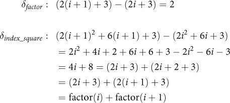
δfactor is easy; the variables cancel and we get the constant 2. But how did we simplify the expression for δindex_square? We observe that by rearranging the terms, we can express it using something we already have, factor(i), and something we need to compute anyway, factor(i + 1). (When you know you need to compute multiple quantities, it’s useful to see if one can be computed in terms of another. This might allow you to do less work.)
With these substitutions, we get our final version of sift; again, our improvements are shown in bold:
Click here to view code image
template <RandomAccessIterator I, Integer N>
void sift(I first, N n) {
I last = first + n;
std::fill(first, last, true);
N i(0);
N index_square(3);
N factor(3);
while (index_square < n) {
// invariant: index_square = 2i^2 + 6i + 3,
// factor = 2i + 3
if (first[i]) {
mark_sieve(first + index_square, last, factor);
}
++i;
index_square += factor;
factor += N(2);
index_square += factor;
}
}
Exercise 3.2. Time the sieve using different data sizes: bit (using std::vector<bool>), uint8_t, uint16_t, uint32_t, uint64_t.
Exercise 3.3. Using the sieve, graph the function
π(n) = number of primes < n
for n up to 107 and find its analytic approximation.
We call primes that read the same backward and forward palindromic primes. Here we’ve highlighted the ones up to 1000:
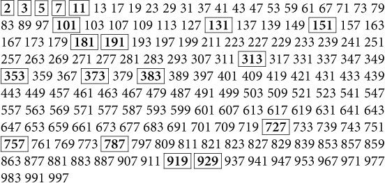
Interestingly, there are no palindromic primes between 1000 and 2000:
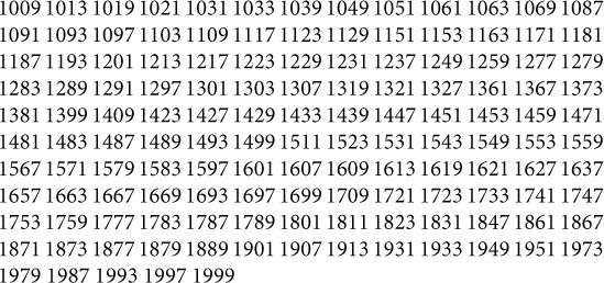
Exercise 3.4. Are there palindromic primes > 1000? What is the reason for the lack of them in the interval [1000, 2000]? What happens if we change our base to 16? To an arbitrary n?
3.4 Perfect Numbers
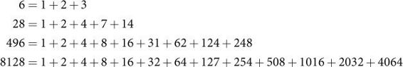
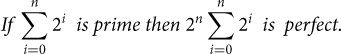
As we saw in Section 3.1, the ancient Greeks were interested in all sorts of properties of numbers. One idea they came up with was that of a perfect number—a number that is the sum of its proper divisors.3 They knew of four perfect numbers:
3 A proper divisor of a number n is a divisor of n other than n itself.
Perfect numbers were believed to be related to nature and the structure of the universe. For example, the number 28 was the number of days in the lunar cycle.
What the Greeks really wanted to know was whether there was a way to predict other perfect numbers. They looked at the prime factorizations of the perfect numbers they knew:
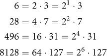
and noticed the following pattern:
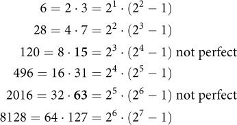
The result of this expression is perfect when the the second term is prime. It was Euclid who presented the proof of this fact around 300 BC.
Theorem 3.3 (Euclid IX, 36):
Useful Formulas
Before we look at the proof, it is useful to remember a couple of algebraic formulas. The first is the difference of powers:
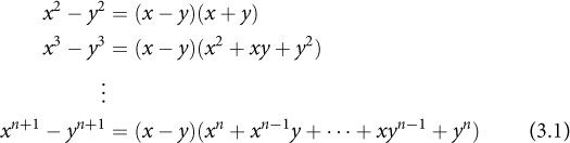
This result can easily be derived using these two equations:
![]()
![]()
The left and right sides of 3.2 and 3.3 are equal by the distributive law. If we then subtract 3.3 from 3.2, we get 3.1.
The second useful formula is for the sum of odd powers:
![]()
which we can derive by converting the sum to a difference and relying on our previous result:
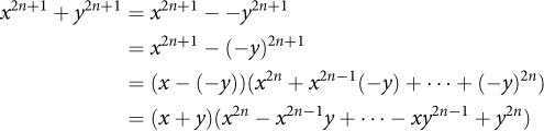
We can get away with this because –1 to an odd power is still –1. We will rely heavily on both of these formulas in the proofs ahead.
Now we know that for n > 0
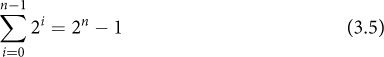
by the difference of powers formula:
2n – 1 = (2 – 1)(2n–1 + 2n–2 + ... + 2 + 1)
(or just think of the binary number you get when you add powers of 2).
Exercise 3.5. Using Equation 3.1, prove that if 2n – 1 is prime, then n is prime.
We are going to prove Euclid’s theorem the way the great German mathematician Carl Gauss did. (We’ll learn more about Gauss in Chapter 8.) First, we will use Equation 3.5, substituting 2n – 1 for both occurrences of ![]() in Euclid’s theorem, to restate the theorem like this:
in Euclid’s theorem, to restate the theorem like this:
If 2n – 1 is prime, then 2n – 1(2n – 1) is perfect.
Next, we define σ(n) to be the sum of the divisors of n. If the prime factorization of n is
![]()
then the set of all divisors consists of every possible combination of the prime divisors raised to every possible power up to ai. For example, 24 = 23 · 31, so the divisors are {20 · 30, 21 · 30, 22 · 30, 20 · 31, 21 · 31, 22 · 31, 23 · 31}. Their sum is
20 · 30 + 21 · 30 + 22 · 30 + 20 · 31 + 21 · 31 + 22 · 31 + 23 · 31 = (20 + 21 + 22 + 23)(30 + 31)
That is, we can write the sum of the divisors for any number n as a product of sums:
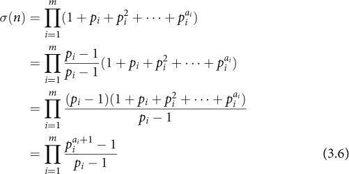
where the last line relies on using the difference of powers formula to simplify the numerator. (In this example, and for the rest of the book, when we use p as an integer variable in our proofs, we assume it’s a prime, unless we say otherwise.)
Exercise 3.6. Prove that if n and m are coprime (have no common prime factors), then
σ(nm) = σ(n)σ(m)
(Another way to say this is that σ is a multiplicative function.)
We now define α(n), the aliquot sum, as follows:
α(n) = σ(n) – n
In other words, the aliquot sum is the sum of all proper divisors of n—all the divisors except n itself.
Now we’re ready for the proof of Theorem 3.3, also known as Euclid IX, 36:
If 2n – 1 is prime, then 2n–1(2n – 1) is perfect.
Proof. Let q = 2n – 1 (2n – 1). We know 2 is prime, and the theorem’s condition is that 2n – 1 is prime, so 2n – 1 (2n – 1) is already a prime factorization of the form ![]() , where m = 2, p1 = 2, a1 = n – 1, p2 = 2n – 1, and a2 = 1. Using the sum of divisors formula (Equation 3.6):
, where m = 2, p1 = 2, a1 = n – 1, p2 = 2n – 1, and a2 = 1. Using the sum of divisors formula (Equation 3.6):
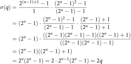
Then
α(q) = σ(q) – q = 2q – q = q
That is, q is perfect.
![]()
We can think of Euclid’s theorem as saying that if a number has a certain form, then it is perfect. An interesting question is whether the converse is true: if a number is perfect, does it have the form 2n–1(2n – 1)? In the 18th century, Euler proved that if a perfect number is even, then it has this form. He was not able to prove the more general result that every perfect number is of that form. Even today, this is an unsolved problem; we don’t know if any odd perfect numbers exist.
Exercise 3.7. Prove that every even perfect number is a triangular number.
Exercise 3.8. Prove that the sum of the reciprocals of the divisors of a perfect number is always 2. Example:
![]()
3.5 The Pythagorean Program
For Pythagoreans, mathematics was not about abstract symbol manipulation, as it is often viewed today. Instead, it was the science of numbers and space—the two fundamental perceptible aspects of our reality. In addition to their focus on understanding figurate numbers (such as square, oblong, and triangular numbers), they believed that there was discrete structure to space. Their challenge, then, was to provide a way to ground geometry in numbers—essentially, to have a unified theory of mathematics based on positive integers.
To do this, they came up with the idea that one line segment could be “measured” by another:
Definition 3.1. A segment V is a measure of a segment A if and only if A can be represented as a finite concatenation of copies of V.
A measure must be small enough that an exact integral number of copies produces the desired segment; there are no “fractional” measures. Of course, different measures might be used for different segments. If one wanted to use the same measure for two segments, it had to be a common measure:
Definition 3.2. A segment V is a common measure of segments A and B if and only if it is a measure of both.
For any given situation, the Pythagoreans believed there is a common measure for all the objects of interest. Therefore, space could be represented discretely.
* * *
Since there could be many common measures, they also came up with the idea of the greatest common measure:
Definition 3.3. A segment V is the greatest common measure of A and B if it is greater than any other common measure of A and B.
The Pythagoreans also recognized several properties of greatest common measure (GCM), which we represent in modern notation as follows:
![]()
![]()
![]()
![]()
Using these properties, they came up with the most important procedure in Greek mathematics—perhaps in all mathematics: a way to compute the greatest common measure of two segments. The computational machinery of the Greeks consisted of ruler and compass operations on line segments. Using C++ notation, we might write the procedure like this, using line_segment as a type:
Click here to view code image
line_segment gcm(line_segment a, line_segment b) {
if (a == b) return a;
if (b < a) return gcm(a - b, b);
/* if (a < b) */ return gcm(a, b - a);
}
This code makes use of the trichotomy law: the fact that if you have two values a and b of the same totally ordered type, then either a = b, a < b, or a > b.
Let’s look at an example. What’s gcm(196, 42)?
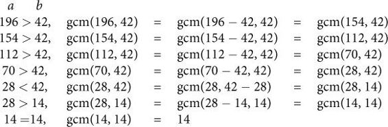
So we’re done: gcm(196, 42) = 14.
Of course, when we say gcm(196, 42), we really mean GCM of segments with length 196 and 42, but for the examples in this chapter, we’ll just use the integers as shorthand.
We’re going to use versions of this algorithm for the next few chapters, so it’s important to understand it and have a good feel for how it works. You may want to try computing a few more examples by hand to convince yourself.
3.6 A Fatal Flaw in the Program
Greek mathematicians found that the well-ordering principle—the fact that any set of natural numbers has a smallest element—provided a powerful proof technique. To prove that something does not exist, prove that if it did exist, a smaller one would also exist.
Using this logic, the Pythagoreans discovered a proof that undermined their entire program.4 We’re going to use a 19th-century reconstruction of this proof by George Chrystal.
4 We don’t know if Pythagoras himself made this discovery, or one of his early followers.
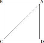
Theorem 3.4: There is no segment that can measure both the side and the diagonal of a square.
Proof. Assume the contrary, that there were a segment that could measure both the side and the diagonal of some square.5 Let us take the smallest such square for this segment:
5 This is an example of proof by contradiction. For more about this proof technique, see Appendix B.1.
Using a ruler and compass,6 we can construct a segment ![]() with the same length as
with the same length as ![]() , and then create a segment starting at F and perpendicular to
, and then create a segment starting at F and perpendicular to ![]() .
.
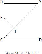
6 Although modern readers may think of a ruler as being used to measure distances, for Euclid it was only a way to draw straight lines. For this reason, some people prefer the term straightedge to describe Euclid’s instrument. Similarly, although a modern compass can be fixed to measure equal distances, Euclid’s compass was used only to draw circles with a given radius; it was collapsible, so it did not preserve distances once lifted.
Now we construct two more perpendicular segments, ![]() and
and ![]() :
:
We know that ∠CFE = 90° (by construction) and that ∠ECF = 45° (since it’s the same as ∠BCA, which is the angle formed by the diagonal of a square, and therefore is half of 90°). We also know that the three angles of a triangle sum to 180°. Therefore
∠CEF = 180° – ∠CFE – ∠ECF = 180° – 90° – 45° = 45°
So ∠CEF = ∠ECF, which means CEF is an isosceles triangle, so the sides opposite equal angles are equal—that is, ![]() . Finally, we add one more segment
. Finally, we add one more segment ![]() :
:
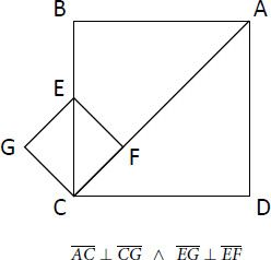
Triangle ABF is also isosceles, with ∠ABF = ∠AFB, since we constructed ![]() . And ∠ABC = ∠AFE, since both were constructed with perpendiculars. So
. And ∠ABC = ∠AFE, since both were constructed with perpendiculars. So
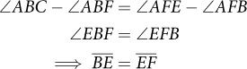
Now, we know ![]() is measurable since that’s part of our premise, and we know
is measurable since that’s part of our premise, and we know ![]() is measurable, since it’s the same as
is measurable, since it’s the same as ![]() , which is also measurable by our premise. So their difference
, which is also measurable by our premise. So their difference ![]() is also measurable. Since we just showed that ΔCEF and ΔBEF are both isosceles,
is also measurable. Since we just showed that ΔCEF and ΔBEF are both isosceles,
![]()
we know ![]() is measurable, again by our premise, and we’ve just shown that
is measurable, again by our premise, and we’ve just shown that ![]() , and therefore
, and therefore ![]() , is measurable. So
, is measurable. So ![]() is measurable.
is measurable.
We now have a smaller square whose side ![]() and diagonal
and diagonal ![]() are both measurable by our common unit. But our original square was chosen to be the smallest for which the relationship held—a contradiction. So our original assumption was wrong, and there is no segment that can measure both the side and the diagonal of a square. If you try to find one, you’ll be at it forever—our line_segment_gcm(a, b) procedure will not terminate.
are both measurable by our common unit. But our original square was chosen to be the smallest for which the relationship held—a contradiction. So our original assumption was wrong, and there is no segment that can measure both the side and the diagonal of a square. If you try to find one, you’ll be at it forever—our line_segment_gcm(a, b) procedure will not terminate.
![]()
To put it another way, the ratio of the diagonal and the side of a square cannot be expressed as a rational number (the ratio of two integers). Today we would say that with this proof, the Pythagoreans had discovered irrational numbers, and specifically that ![]() is irrational.
is irrational.
The discovery of irrational numbers was unbelievably shocking. It undermined the Pythagoreans’s entire program; it meant that geometry could not be grounded in numbers. So they did what many organizations do when faced with bad news: they swore everyone to secrecy. When one of the order leaked the story, legend has it that the gods punished him by sinking the ship carrying him, drowning all on board.
* * *
Eventually, Pythagoras’ followers came up with a new strategy. If they couldn’t unify mathematics on a foundation of numbers, they would unify it on a foundation of geometry. This was the origin of the ruler-and-compass constructions still used today to teach geometry; no numbers are used or needed.
Later mathematicians came up with an alternate, number-theoretic proof of the irrationality of ![]() . One version was included as proposition 117 in some editions of Book X of Euclid’s Elements. While the proof predates Euclid, it was added to Elements some time after the book’s original publication. In any case, it is an important proof:
. One version was included as proposition 117 in some editions of Book X of Euclid’s Elements. While the proof predates Euclid, it was added to Elements some time after the book’s original publication. In any case, it is an important proof:
Theorem 3.5: ![]() is irrational.
is irrational.
Proof. Assume ![]() is rational. Then it can be expressed as the ratio of two integers m and n, where m/n is irreducible:
is rational. Then it can be expressed as the ratio of two integers m and n, where m/n is irreducible:
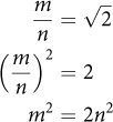
m2 is even, which means that m is also even,7 so we can write it as 2 times some number u, substitute the result into the preceding equation, and do a bit more algebraic manipulation:
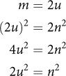
7 This is easily shown: The product of two odd numbers is an odd number, so if m were not even, m2 could not be even. Euclid proved this and many other results about odd and even numbers earlier in Elements.
n2 is even, which means that n is also even. But if m and n are both even, then m/n is not irreducible—a contradiction. So our assumption is false; there is no way to represent ![]() as the ratio of two integers.
as the ratio of two integers.
![]()
3.7 Thoughts on the Chapter
The ancient Greeks’ fascination with “shapes” of numbers and other properties such as prime and perfect were the basis of the mathematical field of number theory. Some of the algorithms they used, such as the Sieve of Eratosthenes, are still very elegant, though we saw how to improve their efficiency further by using some modern optimization techniques.
* * *
Toward the end of the chapter, we saw two different proofs that ![]() is irrational, one geometric and one algebraic. The fact that we have two completely different proofs of the same result is good. It is actually essential for mathematicians to look for multiple proofs of the same mathematical fact, since it increases their confidence in the result. For example, Gauss spent much of his career coming up with multiple proofs for one important theorem, the quadratic reciprocity law.
is irrational, one geometric and one algebraic. The fact that we have two completely different proofs of the same result is good. It is actually essential for mathematicians to look for multiple proofs of the same mathematical fact, since it increases their confidence in the result. For example, Gauss spent much of his career coming up with multiple proofs for one important theorem, the quadratic reciprocity law.
The discovery of irrational numbers emerged from the Pythagoreans’ attempts to represent continuous reality with discrete numbers. While at first glance we might think they were naive to believe that they could accomplish this, computer scientists do the same thing today—we approximate the real world with binary numbers. In fact, the tension between continuous and discrete has remained a central theme in mathematics through the present day, and will probably be with us forever. But rather than being a problem, this tension has actually been the source of great progress and revolutionary insights.