From Mathematics to Generic Programming (2011)
7. Deriving a Generic Algorithm
To generalize something means to think it.
Hegel, Philosophy of Right
In this chapter we’ll take the Egyptian multiplication algorithm from Chapter 2 and, by using the mathematical abstractions introduced in the previous chapter, generalize it to apply to a wide variety of problems beyond simple arithmetic.
7.1 Untangling Algorithm Requirements
Two steps are required to write a good piece of code. The first step is to get the algorithm right. The second step is to figure out which sorts of things (types) it works for. Now, you might be thinking that you already know the type—it’s int or float or whatever you started with. But that may not always be the case; things change. Next year someone may want the code to work with unsigned ints or doubles or something else entirely. We want to design our code so we can reuse it in these different situations.
Let’s take another look at the multiply-accumulate version of the Egyptian multiplication algorithm we developed in Chapter 2. Recall that we are multiplying n by a and accumulating the result in r; also recall that we have a precondition that neither n nor a can be zero:
Click here to view code image
int mult_acc4(int r, int n, int a) {
while (true) {
if (odd(n)) {
r = r + a;
if (n == 1) return r;
}
n = half(n);
a = a + a;
}
}
This time we’ve written some of the code in a slanted typeface and some of it in a bold typeface. Notice that the slanted and bold parts are disjointed; there are no places where a “slanted variable” and a “bold variable” are combined or interact with each other in any way. This means that the requirements for being a slanted variable don’t have to be the same as the requirements for being a bold variable—or to put it in programming language terms, they can be different types.
So what are the requirements for each kind of variable? Until now, we’ve declared the variables as ints, but it seems as if the algorithm would work for many other similar types as well. Slanted variables r and a must be some type that supports adding—we might say that they must be a “plusable” type. The bold variable n must be able to be checked for oddness, compared with 1, and must support division by 2 (it must be “halvable”). Note that division by 2 is a much more restricted operation than division in general. For example, angles can be divided by 2 with ruler-and-compass construction, while dividing them by 3 is impossible in that framework.
We’ve established that r and a are the same type, which we’ll write using the template typename A. Similarly, we said that n is a different type, which we’ll call N. So instead of insisting that all the arguments be of type int, we can now write the following more generic form of the program:
Click here to view code image
template <typename A, typename N>
A multiply_accumulate(A r, N n, A a) {
while (true) {
if (odd(n)) {
r = r + a;
if (n == 1) return r;
}
n = half(n);
a = a + a;
}
}
This makes the problem easier—we can figure out the requirements for A separately from the requirements on N. Let’s dig a bit deeper into these types, starting with the simpler one.
7.2 Requirements on A
What are the syntactic requirements on A? In other words, which operations can we do on things belonging to A? Just by looking at how variables of this type are used in the code, we can see that there are three operations:
• They can be added (in C++, they must have operator+).
• They can be passed by value (in C++, they must have a copy constructor).
• They can be assigned (in C++, they must have operator=).
We also need to specify the semantic requirements. That is, we need to say what these operations mean. Our main requirement is that + must be associative, which we express as follows:
A(T) ![]() ∀a, b, c
∀a, b, c ![]() T : a + (b + c) = (a + b) + c
T : a + (b + c) = (a + b) + c
(In English, we might read the part before the colon like this: “If type T is an A, then for any values a, b, and c in T, the following holds: ....”)
Even though + is associative in theory (and in math generally), things are not so simple on computers. There are real-world cases where associativity of addition does not hold. For example, consider these two lines of code:
w = (x + y) + z;
w = x + (y + z)
Suppose x, y, and z are of type int, and z is negative. Then it is possible that for some very large values, x + y will overflow, while this would not have happened if we added y + z first. The problem arises because addition is not well defined for all possible values of the type int; we say that + is a partial function.
To address this problem, we clarify our requirements. We require that the axioms hold only inside the domain of definition—that is, the set of values for which the function is defined.1
1 For a more rigorous treatment of this topic, see Section 2.1 of Elements of Programming by Stepanov and McJones.
* * *
In fact, there are a couple more syntactic requirements that we missed. They are implied by copy construction and assignment. For example, copy construction means to make a copy that is equal to the original. To do this, we need the ability to test things belonging to A for equality:
• They can be compared for equality (in C++, they must have operator==).
• They can be compared for inequality (in C++, they must have operator!=).
Accompanying these syntactic requirements are semantic requirements for what we call equational reasoning; equality on a type T should satisfy our expectations:
• Inequality is the negation of equality.
(a ≠ b) ![]() ¬(a = b)
¬(a = b)
• Equality is reflexive, symmetric, and transitive.
a = a
a = b ![]() b = a
b = a
a = b ∧ b = c ![]() a = c
a = c
• Equality implies substitutability.
for any function f on T, a = b ![]() f(a) = f(b)
f(a) = f(b)
The three axioms in the middle (reflexivity, symmetry, and transitivity) provide what we call equivalence, but equational reasoning requires something much stronger, so we add the substitutability requirement.
We have a special name for types that behave in the “usual way”—regular types:
Definition 7.1. A regular type T is a type where the relationships between construction, assignment, and equality are the same as for built-in types such as int.
For example:
• T a(b); assert(a == b); unchanged(b);
• a = b; assert(a == b); unchanged(b);
• T a(b); is equivalent to T a; a = b;
For an extensive treatment of regular types, see Chapter 1 of Elements of Programming. All types that we use in this book are regular.
* * *
Now we can formalize the requirements on A:
• Regular type
• Provides associative +
As we saw in Chapter 6, algebraic structures that have a binary associative operation are called semigroups (see Definition 6.5). Also, a regular type guarantees the ability to compare two values for equality, which we need for our associativity axiom. Therefore we can say that A is a semigroup. Its operation is addition, so we might be tempted to call it an additive semigroup. But recall that by convention, additive semigroups are assumed to be commutative. Since we don’t need commutativity for our algorithm, we’ll say that A is a noncommutative additive semigroup. This means that commutativity is not required; it does not mean that commutativity is not allowed. In other words, every (commutative) additive semigroup is also a noncommutative additive semigroup.
Definition 7.2. A noncommutative additive semigroup is a semigroup where the associative binary operation is +.
Some examples of noncommutative additive semigroups are positive even integers, negative integers, real numbers, polynomials, planar vectors, Boolean functions, and line segments. These examples happen to also be additive semigroups, but that is not always the case. As we shall see, + may have different interpretations for these different types, but it will always be associative.
For many centuries, the symbol “+” has been used, by convention, to mean a commutative operation as well as an associative one. Many programming languages (e.g., C++, Java, Python) use + for string concatenation, a noncommutative operation. This violates standard mathematical practice, which is a bad idea. The mathematical convention is as follows:
• If a set has one binary operation and it is both associative and commutative, call it +.
• If a set has one binary operation and it is associative and not commutative, call it *.
20th-century logician Stephen Kleene introduced the notation ab to denote string concatenation (since in mathematics * is usually elided).
The Naming Principle
If we are coming up with a name for something, or overloading an existing name, we should follow these three guidelines:
1. If there is an established term, use it.
2. Do not use an established term inconsistently with its accepted meaning. In particular, overload an operator or function name only when you will be preserving its existing semantics.
3. If there are conflicting usages, the much more established one wins.
The name vector in STL was taken from the earlier programming languages Scheme and Common Lisp. Unfortunately, this was inconsistent with the much older meaning of the term in mathematics and violates Rule 3; this data structure should have been called array. Sadly, if you make a mistake and violate these principles, the result might stay around for a long time.
7.3 Requirements on N
Now that we know that A must be a noncommutative additive semigroup, we can specify that in our template instead of just saying typename:
Click here to view code image
template <NoncommutativeAdditiveSemigroup A, typename N>
A multiply_accumulate(A r, N n, A a) {
while (true) {
if (odd(n)) {
r = r + a;
if (n == 1) return r;
}
n = half(n);
a = a + a;
}
}
Here we’re using NonCommutativeAdditiveSemigroup as a C++ concept, a set of requirements on types that we’ll discuss in Chapter 10. Instead of saying typename, we name the concept we wish to use. Since concepts are not yet supported in the language as of this writing, we’re doing a bit of preprocessor slight-of-hand:
Click here to view code image
#define NonCommutativeAdditiveSemigroup typename
As far as the compiler is concerned, A is just a typename, but for us, it’s a NonCommutativeAdditiveSemigroup. We’ll use this trick from now on when we want to specify the type requirements in templates.
Although this behavior is not needed for abstract mathematics, in programming we need our variables to be constructible and assignable, which are also guaranteed by being regular types. From now on, when we specify an algebraic structure as a concept, we will assume that we are inheriting all of the regular type requirements.
What about the requirements on our other argument’s type, N? Let’s start with the syntactic requirements. N must be a regular type implementing
• half
• odd
• == 0
• == 1
Here are the semantic requirements on N:
• even(n) ![]() half(n) + half(n) = n
half(n) + half(n) = n
• odd(n) ![]() even(n – 1)
even(n – 1)
• odd(n) ![]() half(n – 1) = half(n)
half(n – 1) = half(n)
• Axiom: n ≤ 1 ∨ half(n) = 1 ∨ half(half(n)) = 1 ∨ . . .
Which C++ types satisfy these requirements? There are several: uint8_t, int8_t, uint64_t, and so on. The concept that they satisfy is called N Integer.
* * *
Now we can finally write a fully generic version of our multiply-accumulate function by specifiying the correct requirements for both types:
Click here to view code image
template <NoncommutativeAdditiveSemigroup A, Integer N>
A multiply_accumulate_semigroup(A r, N n, A a) {
// precondition(n >= 0);
if (n == 0) return r;
while (true) {
if (odd(n)) {
r = r + a;
if (n == 1) return r;
}
n = half(n);
a = a + a;
}
}
We’ve added one more line of code, which returns r when n is zero. We do this because when n is zero, we don’t need to do anything. However, the same is not true for multiply, as we’ll see in a moment.
Here’s the multiply function that calls the preceding code; it has the same requirements:
Click here to view code image
template <NoncommutativeAdditiveSemigroup A, Integer N>
A multiply_semigroup(N n, A a) {
// precondition(n > 0);
while (!odd(n)) {
a = a + a;
n = half(n);
}
if (n == 1) return a;
return multiply_accumulate_semigroup(a, half(n - 1), a + a);
}
We can also update our helper functions odd and half to work for any Integer:
Click here to view code image
template <Integer N>
bool odd(N n) { return bool(n & 0x1); }
template <Integer N>
N half(N n) { return n >> 1; }
7.4 New Requirements
Our precondition for multiply says that n must be strictly greater than zero. (We made this assumption earlier, since the Greeks had only positive integers, but now we need to make it explicit.) What should an additive semigroup multiplication function return when n is zero? It should be the value that doesn’t change the result when the semigroup operator—addition—is applied. In other words, it should be the additive identity. But an additive semigroup is not required to have an identity element, so we can’t depend on this property. In other words, we can’t rely on there being an equivalent of zero. (Remember, a no longer has to be an integer; it can be any NoncommutativeAdditiveSemigroup, such as positive integers or nonempty strings.) That’s why n can’t be zero.
But there is an alternative: instead of having a restriction on the data requiring n > 0, we can require that any type we use know how to deal with 0. We do this by changing the concept requirement on n from additive semigroup to monoid. Recall from Chapter 6 that in addition to an associative binary operation, a monoid contains an identity element e and an identity axiom that says
x ο e = e ο x = x
In particular, we’re going to use a noncommutative additive monoid, where the identity element is called “0”:
x + 0 = 0 + x = x
This is the multiply function for monoids:
Click here to view code image
template <NoncommutativeAdditiveMonoid A, Integer N>
A multiply_monoid(N n, A a) {
// precondition(n >= 0);
if (n == 0) return A(0);
return multiply_semigroup(n, a);
}
What if we want to allow negative numbers when we multiply? We need to ensure that “multiplying by a negative” makes sense for any type we might have. This turns out to be equivalent to saying that the type must support an inverse operation. Again, we find that our current requirement—noncommutative additive monoid—is not guaranteed to have this property. For this, we need a group. A group, as you may recall from Chapter 6, includes all of the monoid operations and axioms, plus an inverse operation x–1 that obeys the cancellation axiom
x ο x–1 = x–1 ο x = e
In our case, we want a noncommutative additive group, one where the inverse operation is unary minus and the cancellation axiom is:
x+ –x = –x + x = 0
Having strengthened our type requirements, we can remove our preconditions on n to allow negative values. Again, we’ll wrap the last version of our function with our new one:
Click here to view code image
template <NoncommutativeAdditiveGroup A, Integer N>
A multiply_group(N n, A a) {
if (n < 0) {
n = -n;
a = -a;
}
return multiply_monoid(n, a);
}
7.5 Turning Multiply into Power
Now that our code has been generalized to work for any additive semigroup (or monoid or group), we can make a remarkable observation:
If we replace + with * (thereby replacing doubling with squaring), we can use our existing algorithm to compute an instead of n · a.
Here’s the C++ function we get when we apply this transformation to our code for multiply_accumulate_semigroup:
Click here to view code image
template <MultiplicativeSemigroup A, Integer N>
A power_accumulate_semigroup(A r, A a, N n) {
// precondition(n >= 0);
if (n == 0) return r;
while (true) {
if (odd(n)) {
r = r * a;
if (n == 1) return r;
}
n = half(n);
a = a * a;
}
}
The new function computes ran. The only things that have changed are highlighted in bold. Note that we’ve changed the order of arguments a and n, so as to match the order of arguments in standard mathematical notation (i.e., we say na, but an).
Here’s the function that computes power:
Click here to view code image
template <MultiplicativeSemigroup A, Integer N>
A power_semigroup(A a, N n) {
// precondition(n > 0);
while (!odd(n)) {
a = a * a;
n = half(n);
}
if (n == 1) return a;
return power_accumulate_semigroup(a, a * a, half(n - 1));
}
Here are the wrapped versions for multiplicative monoids and groups:
Click here to view code image
template <MultiplicativeMonoid A, Integer N>
A power_monoid(A a, N n) {
// precondition(n >= 0);
if (n == 0) return A(1);
return power_semigroup(a, n);
}
template <MultiplicativeGroup A, Integer N>
A power_group(A a, N n) {
if (n < 0) {
n = -n;
a = multiplicative_inverse(a);
}
return power_monoid(a, n);
}
Just as we needed an additive identity (0) for our monoid multiply, so we need a multiplicative identity (1) in our monoid power function. Also, just as we needed an additive inverse (unary minus) for our group multiply, so we need a multiplicative inverse for our group power function. There’s no built-in multiplicative inverse (reciprocal) operation in C++, but it’s easy to write one:
Click here to view code image
template <MultiplicativeGroup A>
A multiplicative_inverse(A a) {
return A(1) / a;
}
7.6 Generalizing the Operation
We’ve seen examples of two semigroups—additive and multiplicative—each with its associated operation (+ and *, respectively). The fact that we could use the same algorithm for both is wonderful, but it was annoying to have to write different versions of the same code for each case. In reality, there could be many such semigroups, each with its associative operations (for example, multiplication mod 7) that work on the same type T. Rather than having another version for every operation we want to use, we can generalize the operation itself, just as we generalized the types of the arguments before. In fact, there are many situations where we need to pass an operation to an algorithm; you may have seen examples of this in STL.
Here’s the accumulate version of our power function for an arbitrary semigroup. We still refer to the function it computes as “power,” even though the operation it’s repeatedly applying may not necessarily be multiplication.
Click here to view code image
template <Regular A, Integer N, SemigroupOperation Op>
// requires (Domain<Op, A>)
A power_accumulate_semigroup(A r, A a, N n, Op op) {
// precondition(n >= 0);
if (n == 0) return r;
while (true) {
if (odd(n)) {
r = op(r, a);
if (n == 1) return r;
}
n = half(n);
a = op(a, a);
}
}
Notice that we’ve added a “requires” comment to our template that says the domain of operation Op must be A. If future versions of C++ support concepts, this comment could be turned into a statement (similar to an assertion) that the compiler could use to ensure the correct relationship holds between the given types. As it is, we’ll have to make sure as programmers that we call this function only with template arguments that satisfy the requirement.
Also, since we no longer know which kind of semigroup to make A—it could be additive, multiplicative, or something else altogether, depending on Op—we can require only that A be a regular type. The “semigroupness” will come from the requirement that Op be a SemigroupOperation.
We can use this function to write a version of power for an arbitrary semigroup:
Click here to view code image
template <Regular A, Integer N, SemigroupOperation Op>
// requires (Domain<Op, A>)
A power_semigroup(A a, N n, Op op) {
// precondition(n > 0);
while (!odd(n)) {
a = op(a, a);
n = half(n);
}
if (n == 1) return a;
return power_accumulate_semigroup(a, op(a, a),
half(n - 1), op);
}
As we did before, we can extend the function to monoids by adding an identity element. But since we don’t know in advance which operation will be passed, we have to obtain the identity from the operation:
Click here to view code image
template <Regular A, Integer N, MonoidOperation Op>
// requires(Domain<Op, A>)
A power_monoid(A a, N n, Op op) {
// precondition(n >= 0);
if (n == 0) return identity_element(op);
return power_semigroup(a, n, op);
}
Here are examples of identity_element functions for + and *:
Click here to view code image
template <NoncommutativeAdditiveMonoid T>
T identity_element(std::plus<T>) { return T(0); }
template <MultiplicativeMonoid T>
T identity_element(std::multiplies<T>) { return T(1); }
Each of these functions specifies the type of the object it expects to be called with, but doesn’t name it, since the object is never used. The first one says, “The additive identity is 0.” Of course, there will be different identity elements for different monoids—for example, the maximum value of the type T for min.
* * *
To extend power to groups, we need an inverse operation, which is itself a function of the specified GroupOperation:
Click here to view code image
template <Regular A, Integer N, GroupOperation Op>
// requires(Domain<Op, A>)
A power_group(A a, N n, Op op) {
if (n < 0) {
n = -n;
a = inverse_operation(op)(a);
}
return power_monoid(a, n, op);
}
Examples of inverse_operation look like this:
Click here to view code image
template <AdditiveGroup T>
std::negate<T> inverse_operation(std::plus<T>) {
return std::negate<T>();
}
template <MultiplicativeGroup T>
reciprocal<T> inverse_operation(std::multiplies<T>) {
return reciprocal<T>();
}
STL already has a negate function, but (due to an oversight) has no reciprocal. So we’ll write our own. We’ll use a function object—a C++ object that provides a function declared by operator() and is invoked like a function call, using the name of the object as the function name. To learn more about function objects, see Appendix C.
Click here to view code image
template <MultiplicativeGroup T>
struct reciprocal {
T operator()(const T& x) const {
return T(1) / x;
}
};
This is just a generalization of the multiplicative_inverse function we wrote in the previous section.2
2 This time we do not need a precondition preventing x from being zero, because MultiplicativeGroup does not contain a non-invertible zero element. If in practice we have a type such as double that otherwise would satisfy the requirements of MultiplicativeGroup if it did not contain a zero, we can add a precondition to eliminate that case.
Reduction
The power algorithm is not the only important algorithm defined on semigroups. Another key algorithm is reduction, in which a binary operation is applied successively to each element of a sequence and its previous result.
Two commonly seen examples of this in mathematics are the summation (∑) function for additive semigroups and the product (∏) function for multiplicative semigroups. We can generalize this to an arbitrary semigroup.
This generalized version of reduction was invented in 1962 by computer scientist Ken Iverson in his language APL. In APL terminology, the / represented the reduction operator. For example, summation of a sequence is expressed as
+ / 1 2 3
The idea of reduction has appeared in many contexts since then. John Backus, inventor of the first high-level programming language, included a similar operator called insert in his language FP in 1977. (He called operators “functional forms.”) An early paper on generic programming, “Operators and Algebraic Structures,” by Kapur, Musser, and Stepanov, extended the idea to parallel reduction in 1981 and clarified the relationship to associative operations. The language Common Lisp, popular in the 1980s for artificial intelligence applications, included a reduce function. Google’s MapReduce system, and its open-source variant Hadoop, is a current practical application of these ideas.
7.7 Computing Fibonacci Numbers
Note: This section assumes some basic knowledge of linear algebra. The rest of the book does not depend on the material covered here, and this section may be skipped without affecting the reader’s understanding.
In Chapter 4 we met the early 13th-century mathematician Leonardo Pisano, often known today as Fibonacci. One of the things he’s best known for is a famous problem he posed: if we start with one pair of rabbits, how many pairs will we have after a certain number of months? To simplify the problem, Leonardo made some assumptions: the original pair of rabbits and every litter afterward consists of a male and a female; female rabbits take one month to reach sexual maturity and have one litter per month after that; rabbits live forever.
Initially we have 1 pair of rabbits. At the start of month 2, the rabbits mate, but we still have only 1 pair. At the start of month 3, the female gives birth, so we have 2 pairs. At the start of month 4, the initial female gives birth another time, so we have 3 pairs. At the start of month 5, the initial female gives birth again, but so does the female born in month 3, so now we have 5 pairs, and so on. If we say that we had 0 rabbits in month 0 (before the experiment began), then the number of pairs in each month looks like this:
0, 1, 1, 2, 3, 5, 8, 13, 21, 34...
Each month’s population can be obtained simply by adding the populations of each of the previous two months. Today, elements of this sequence are called Fibonacci numbers, and such a sequence is defined formally like this:
F0 = 0
F1 = 1
Fi = Fi–1 + Fi–2
How long does it take to compute the nth Fibonacci number? The “obvious” answer is n – 2, but the obvious answer is wrong.
The naive way to implement this in C++ is something like this:
Click here to view code image
int fib0(int n) {
if (n == 0) return 0;
if (n == 1) return 1;
return fib0(n - 1) + fib0(n - 2);
}
However, this code does an awful lot of repeated work. Consider the calculations to compute fib0(5):
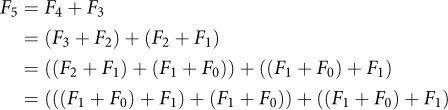
Even in this small example, the computation does 17 additions, and just the quantity F1 + F0 is recomputed 5 times.
Exercise 7.1. How many additions are needed to compute fib0(n)?
Recomputing the same thing over and over is unacceptable, and there’s no excuse for code like that. We can easily fix the code by keeping a running state of the previous two results:
Click here to view code image
int fibonacci_iterative(int n) {
if (n == 0) return 0;
std::pair<int, int> v = {0, 1};
for (int i = 1; i < n; ++i) {
v = {v.second, v.first + v.second};
}
return v.second;
}
This is an acceptable solution, which takes O(n) operations. In fact, given that we want to find the nth element of a sequence, it might appear to be optimal. But the amazing thing is that we can actually compute the nth Fibonacci number in O(log n) operations, which for most practical purposes is less than 64.
Suppose we represent the computation of the next Fibonacci number from the previous two using the following matrix equation:3
![]()
3 A brief refresher on matrix multiplication may be found at the beginning of Section 8.5.
Then the nth Fibonacci number may be obtained by
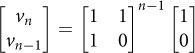
In other words, we can compute the nth Fibonacci number by raising a certain matrix to a power. As we will see, matrix multiplication can be used to solve many problems. Matrices are a multiplicative monoid, so we already have an O(log n) algorithm—our power algorithm from Section 7.6.
Exercise 7.2. Implement computing Fibonacci numbers using power.
This is a nice application of our power algorithm, but computing Fibonacci numbers isn’t the only thing we can do. If we replace the + with an arbitrary linear recurrence function, we can use the same technique to compute any linear recurrence.
Definition 7.3. A linear recurrence function of order k is a function f such that
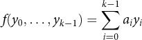
Definition 7.4. A linear recurrence sequence is a sequence generated by a linear recurrence from initial k values.
The Fibonacci sequence is a linear recurrence sequence of order 2.
For any linear recurrence sequence, we can compute the nth step by doing matrix multiplication using our power algorithm:
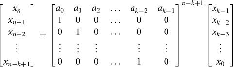
The line of 1s just below the diagonal provides the “shifting” behavior, so that each value in the sequence depends on the previous k.
7.8 Thoughts on the Chapter
We began this chapter by analyzing the requirements on our code from Chapter 2, abstracting the algorithms to use an associative operation on arbitrary types. We were able to rewrite the code so that it is defined on certain algebraic structures: semigroups, monoids, and groups.
Next, we demonstrated that the algorithm could be generalized, first from multiplication to power, then to arbitrary operations on our algebraic structures. We’ll use this generalized power algorithm again later on in the book.
The process we went through—taking an efficient algorithm, generalizing it (without losing efficiency) so that it works on abstract mathematical concepts, and then applying it to a variety of situations—is the essence of generic programming.