Network Security Through Data Analysis: Building Situational Awareness (2014)

Part III. Analytics

Chapter 13. Graph Analysis

A graph is a mathematical construct composed of one or more nodes (or vertices) connected together by one or more links (or edges). Graphs are an effective way to describe communication without getting lost in the weeds. They can be used to model connectivity and provide a comprehensive view of that connectivity while abstracting away details such as packet sizes and session length. Additionally, graph attributes such as centrality can be used to identify critical nodes in a network. Finally, many important protocols (in particular, SMTP and routing) rely on algorithms that model their particular network as a graph.

The remainder of this chapter is focused on the analytic properties of graphs. We begin by describing what a graph is and then developing examples for major attributes: shortest paths, centrality, clusters, and clustering coefficient.

Graph Attributes: What Is a Graph?

A graph is a mathematical representation of a collection of objects and their interrelationships. Originally developed in 1736 by Leonhard Euler to address the problem of crossing the bridges of Konigsberg, graphs have since been used to model everything from the core members of conspiracies to the frequency of sounds uttered in the English language. Graphs are an extremely powerful and flexible descriptive tool, and that power comes because they are extremely fungible. Researchers in mathematics, engineering, and sociology have developed an extensive set of constructed and observed graph attributes that can be used to model various behaviors. The first challenge in using graphs is deciding which attributes you need and how to derive them. The following attributes represent a subset of what can be done with graphs, and are chosen for their direct relevance to the traffic models built later. Any good book on graph theory will include more attributes because at some point, someone has tried just about anything with a graph.

At the absolute minimum, a graph is composed of nodes and links, where a link is a connection between exactly two nodes. A link can be directed or undirected; if a link is directed, then it has an origin and a destination. Conventionally, a graph is either composed entirely of directed links, or entirely of undirected links. If a graph is undirected, then each node has a degree, which is the number of links connected to that node. Nodes in a directed graph have an indegree, which is the number of links with a destination that is that node, and an outdegree, which is the number of links whose origin is the node.

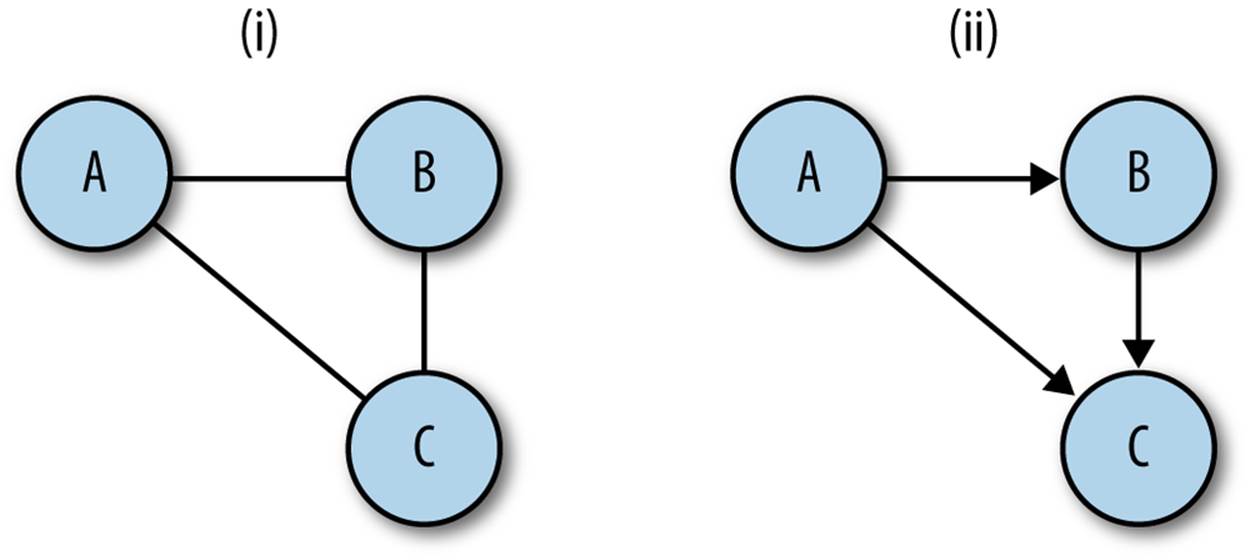
Figure 13-1. Directed and undirected graphs: in (i), the graph is undirected and each node has degree 2; in (ii), the graph is directed: node a has outdegree 2, indegree 0; node b has outdegree 1, indegree 1; node c has outdegree 0, indegree 2

In network traffic logs, there are a number of candidates for conversion to graphs. In flow data, IP addresses can be used as nodes and the existence of a flow between them can be used as links. In HTTP server logs, nodes can be individual pages linked together by Referer headers. In mail logs, email addresses can be nodes, and the links between them can be expressed as mail. Anything expressed as a communication from point A to point B is a suitable candidate.

A disclaimer about code in this section of the book: it is intended primarily for educational purposes, so in the interests of clearly pointing out how various algorithms or numbers work, I’ve avoided optimization and a lot of the exception trapping I’d use in production code. This is particularly important when dealing with graph analysis, since graph algorithms are notoriously expensive. There are a number of good libraries available for doing graph analysis, and they will process complex graphs much more efficiently than anything I hack together here.

The script in Example 13-1 can create directed or undirected graphs from lists of pairs (for example, the output of rwcut --field=1,2 --no-title --delim=' '). There are a couple of methods under the hood for implementing graphs; in this case, I’m using adjacency lists, which I feel are the most intuitively obvious. In an adjacency list implementation, each node maintains a table of all the links adjacent to it.

Example 13-1. Basic graphs

#!/usr/bin/env python

#

# basic_graph.py

#

# Library

# Provides:

# Graph Object, which as a constructor takes a flow file

#

import os, sys

class UndirGraph:

""" An undirected, unweighted graph class. This also serves as the base class

for all other graph implementations in this chapter """

def add_node(self, node_id):

self.nodes.add(node_id)

def add_link(self, node_source, node_dest):

self.add_node(node_source)

self.add_node(node_dest)

if not self.links.has_key(node_source):

self.links[node_source] = {}

self.links[node_source][node_dest] = 1

if not self.links.has_key(node_dest):

self.links[node_dest] = {}

self.links[node_dest][node_source] = 1

return

def count_links(self):

total = 0

for i in self.links.keys():

total += len(self.links[i].keys())

return total/2 # Compensating for link doubling in undirected graph

def neighbors(self, address):

# Returns a list of all the nodes adjacent to the node address,

# returns an empty list of there are no ndoes (technically impossible with

# these construction rules, but hey).

if self.nodes.has_key(address):

return self.links[address].keys()

else:

return None

def __str__(self):

return 'Undirected graph with %d nodes and %d links' % (len(self.nodes),

self.count_links())

def adjacent(self, sip, dip):

# Note, we've defined the graph as undirected during construction,

# consequently links only has to return the source.

if self.links.has_key(sip):

if self.links[sip].has_key(dip):

return True

def __init__(self):

#

# This graph is implemented using adjacency lists; every node has

# a key in the links hashtable, and the resulting value is another hashtable.

#

# The nodes table is redundant for undirected graphs, since the existence of

# a link between X and Y implies a link between Y and X, but in the case of

# directed graphs it'll providea speedup if I'm just looking for a

# particular node.

self.links = {}

self.nodes = set()

class DirGraph(UndirGraph):

def add_link(self, node_source, node_dest):

# Note that in comparison to the undirected graph, we only

# add links in one direction

self.add_node(node_source)

self.add_node(node_dest)

if not self.links.has_key(node_source):

self.links[node_source] = {}

self.links[node_source][node_dest] = 1

return

def count_links(self):

# This had to be changed from the original count_links since I'm now

# using an undirected graph.

total = 0

for i in self.links.keys():

total += len(self.links[i].keys())

return total

if __name__ == '__main__':

#

# This is a stub executable that will create and then render an

# undirected graph assuming that it receives some kind of

# space delimited set of (source, dest) pairs on input

#

a = sys.stdin.readlines()

tgt_graph = DirGraph()

for i in a:

source, dest = i.split()[0:2]

tgt_graph.add_link(source, dest)

print tgt_graph

print "Links:"

for i in tgt_graph.links.keys():

dest_links = ' '.join(tgt_graph.links[i].keys())

print '%s: %s' % (i, dest_links)

GRAPH CONSTRUCTION VERSUS GRAPH ATTRIBUTES

It’s really tempting when working with graphs to start creating complicated relations between network attributes to graph attributes, such as deciding direction points from client to server, or weighting links with the traffic between nodes.

I have found that constructions are more trouble than they’re worth. It’s better to start with a simple graph and examine its attributes rather than try to build up a complicated graph representation. With that in mind, two rules for converting raw data into graphs:

Define communication

A link should represent a communication between two nodes; with flow data that may mean that a link only occurs when the flow has 10 or more packets and an ACK flag high in order to throw out scanning and failed login attempts.

Define node identity

Should IP addresses be a node, or IP addresses and ports in combination? I’ve found it useful to split the ports into services (everything under 1024 is unique; everything above that is client) and then use an IP:service combination.

Labeling, Weight, and Paths

On a graph, a path is a set of links connecting two nodes. In a directed graph, paths follow the direction of the link, while in an undirected graph they can move in either direction. Of particular importance in graph analysis are shortest paths, which as the name implies are the shortest set of links required to get from point A to point B (see Example 13-2).

Example 13-2. An shortest path algorithm

#!/usr/bin/env python

#

# apsp.py -- implemented weighted paths and dijkstra's algorithm

import sys,os,basic_graph

class WeightedGraph(basic_graph.UndirGraph):

def add_link(self, node_source, node_dest, weight):

# Weighted bidirectional link aid, note that

# we keep the aa, but now instead of simply setting the value to

# 1, we add the weight value. This reverts to an unweighted

# graph if we always use the same weight.

self.add_node(node_source)

self.add_node(node_dest)

if not self.links.has_key(node_source):

self.links[node_source] = {}

if not self.links[node_source].has_key(node_dest):

self.links[node_source][node_dest] = 0

self.links[node_source][node_dest] += weight

if not self.links.has_key(node_dest):

self.links[node_dest] = {}

if not self.links[node_dest].has_key(node_source):

self.links[node_dest][node_source] = 0

self.links[node_dest][node_source] += weight

def dijkstra(self, node_source):

# Given a source node, create a map of paths for each vertex

D = {} # Tentative distnace table

P = {} # predecessor table

# The predecessor table exploits a unique feature of shortest paths,

# every subpath of a shortest path is itself a shortest path, so if

# you find that (B,C,D) is the shortest path from A to E, then

# (B,C) is the shortest path from A to D. All you have to do is keep

# track of the predecessor and walk backwards.

infy = 999999999999 # Shorthand for infinite

for i in self.nodes:

D[i] = infy

P[i] = None

D[node_source] = 0

node_list = list(self.nodes)

while node_list != []:

current_distance = infy

current_node = None

# Step 1, find the node with the smallest distance, that'll

# be node_source in the first call as it's the only one

# where D =0

for i in node_list:

if D[i] < current_distance:

current_distance = D[i]

current_node = i

node_index = node_list.index(i)

del node_list[node_index] # Remove it from the list

if current_distance == infy:

break # We've exhausted all paths from the node,

# everything else is in a different component

for i in self.neighbors(current_node):

new_distance = D[current_node] + self.links[current_node][i]

if new_distance < D[i]:

D[i] = new_distance

P[i] = current_node

node_list.insert(0, i)

for i in D.keys():

if D[i] == infy:

del D[i]

for i in P.keys():

if P[i] is None:

del P[i]

return D,P

def apsp(self):

# Calls dijkstra repeatedly to create an all-pairs shortest paths table

apsp_table = {}

for i in self.nodes:

apsp_table[i] = self.dijkstra(i)

return apsp_table

An alternative formulation of shortest paths uses weighting. In a weighted graph, links are assigned a numeric weight. When weight is assigned, the shortest path is no longer simply the smallest number of connected links from point A to point B, but the set of links whose total weight is smallest. Figure 13-2 shows these attributes in more detail.

Shortest paths are a fundamental building block in graph analysis. In most routing services, such as Open Shortest Path First (OSPF), finding shortest paths is the goal. As a result, a good number of graph analyses begin by building a table of shortest paths between all the nodes using an All Pairs, Shortest Paths (APSP) algorithm on the graph in order to create a table of all of them. The code in the following sidebar provides an example of using Dijkstra’s Algorithm on a weighted, undirected, graph to calculate shortest paths.

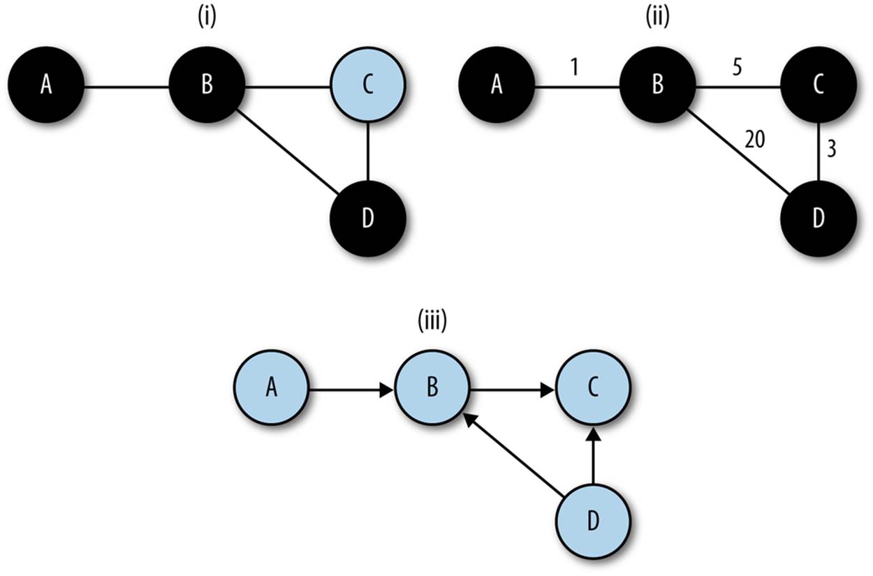
Figure 13-2. Weighting and paths, the shortest path from a to d: (i) in an undirected, unweighted graph, the shortest path involves the least nodes, (ii) in a weighted graph, the shortest path generally has the lowest total weight, (iii) in a directed graph, the shortest path might not be achievable

Dijkstra’s algorithm is a good shortest path algorithm that can handle any graph whose link weights are positive. Shortest path algorithms are critical in a number of fields, and there are consequently a huge number of algorithms available depending on the structure of the graph, the construction of the nodes, and the amount of knowledge of the graph that the individual nodes have.

Shortest paths effectively define the distance between nodes on a graph, and serve as the building blocks for a number of other attributes. Of particular importance are centrality attributes (see Example 13-3). Centrality is a concept originating in social network analysis; social network analysis models the relationships between entities using graphs and mines the graphs for attributes showing the relationship between these entities in bulk. Centrality, for which there are several measures, is an indicator of how important a node is to that graph’s structure.

Example 13-3. Centrality calculation

#/usr/bin/env python

#

#

# centrality.py

#

# script which generates centrality statistics for a dataset

#

# input:

# A table of pairs in the form source, destination with a space separating them

# Weight is implicit, the weight of a link is the number of times a pair appears

#

# command_line

# calc_centrality.py n

# n: integer value, the number of elements to return in the report

#

# Output

# 7 Column report of the form rank | betweenness winner | betweenness

# score | degree winner | degree score | closeness winner | closeness

# score

import sys,string

import apsp

n = int(sys.argv[1])

closeness_results = []

degree_results = []

betweenness_results = []

target_graph = apsp.WeightedGraph()

# load up the graph

for i in sys.stdin.readlines():

source, dest = i[:-1].split()

target_graph.add_link(source, dest, 1)

# Calculate degree centrality; the easiest of the bunch since it's just the

# degree

for i in target_graph.nodes:

degree_results.append((i, len(target_graph.neighbors(i))))

apsp_results = target_graph.apsp()

# Now, calculate the closeness centrality scores

for i in target_graph.nodes:

dt = apsp_results[i][0] # This is the distance table

total_distance = reduce(lambda a,b:a+b, dt.values())

closeness_results.append((i, total_distance))

# Now, we calcualte betweenness centrality scores

bt_table = {}

for i in target_graph.nodes:

bt_table[i] = 0

for current_node in target_graph.nodes:

# Reconstruct the shortest paths from the predecessor table;

# for every entry in the distance table, walk backwards from that

# entry to the correspending origin to get the shortest path, then

# count the nodes in that path on the master bt table

pred_table = apsp_results[i][1] # We have the predecessor table

sp_list = apsp_results[i][0]

if current_node in sp_list.keys():

path = []

for working_node in sp_list.keys():

if working_node != current_node:

# We should be done with working node at this point, count

# the nodes there for bt score

for i in path:

bt_table[i] += 1

else:

path.append(working_node)

working_node = pred_table[working_node]

for i in bt_table.keys():

betweenness_results.append((i,bt_table[i]))

# Order the tables, remember that betweenness and degree use higher score, closeness

# lower score

degree_results.sort(lambda a,b:b[1]-a[1])

betweenness_results.sort(lambda a,b:b[1]-a[1])

closeness_results.sort(lambda a,b:a[1]-b[1])

print "%5s|%15s|%10s|%15s|%10s|%15s|%10s" %

("Rank", "Between", "Score", "Degree", "Score","Close", "Score")

for i in range(0, n):

print "%5d|%15s|%10d|%15s|%10d|%15s|%10d" % ( i + 1,

str(betweenness_results[i][0]),

betweenness_results[i][1],

str(degree_results[i][0]),

degree_results[i][1],

str(closeness_results[i][0]),

closeness_results[i][1])

We’re going to consider three metrics for centrality in this book: degree, closeness, and betweenness. Degree is the simplest centrality measure; in an undirected graph, the degree centrality of a node is the node’s degree.

Closeness and betweenness centrality are both associated with shortest paths. The closeness centrality represents the ease of transmitting information from a particular node to any other node on the graph. To calculate the closeness of a node, you calculate the sum total distance between that node and every other node in the graph. The node with the lowest total value has the highest closeness centrality.

Like closeness centrality, betweenness centrality is a function of the shortest paths. Betweenness centrality repersents the likelihood that a node will be part of the shortest path between any two particular nodes. Betweenness centrality is calculated by generating a table of all the shortest paths and then counting the number of paths using that node.

Centrality algorithms are all relative measures. Operationally, they’re generally best used as ranking algorithms. For example, finding that a particular web page has a high betweenness centrality means that most users when surfing are going to visit that page, possibly because it’s a gatekeeper or an important index. Observing user surfing patterns and finding that a particular node has a high closeness centrality can be useful for identifying important news or information sites.

Components and Connectivity

If two nodes in an undirected graph have a path between them, then they are connected. The set of all nodes that have paths to each other composes a connected component. In directed graphs, the corresponding terms are weakly connected (if the paths exist when direction is ignored), andstrongly connected (if the paths exist when direction is accounted for).

A graph can be broken into its components by using a breadth-first search. A breadth-first search (BFS) is a search that progresses by picking a node, examining all the neighbors of that node, and then examining each of those neighbors in turn. This contrasts with a depth-first search (DFS), which examines a single neighbor, then a neighbor of that neighbor, and so on. The code in Example 13-4 shows how to use a breadth-first search to break a graph into components.

Example 13-4. Calculating components and clustering coefficient

#!/usr/bin/env python

#

#

import os,sys, basic_graph

def calculate_components(g):

# Creates a table of components via a breadth first search.

component_table = {}

unfinished_nodes = {}

for i in g.nodes.keys():

unfinished_nodes[i] = 1

node_list = [g.nodes.keys()[0]]

component_index = 1

while node_list != []:

current_node = node_list[0]

del node_list[0]

del unfinished_nodes[current_node]

for i in g.neighbors(current_node):

component_table[i] = component_index

node_list.insert(0, i)

if node_list == [] and len(unfinished_nodes) > 0:

node_list = [unfinished_nodes.keys()[0]]

return component_table

Clustering Coefficient

Another mechanism for measuring the relationship between nodes on a graph is the clustering coefficient. The clustering coefficient is the probability that any two neighbors of a particular node on a graph are neighbors of each other. Example 13-5 shows a code snippet for calculating the clustering coefficient.

Example 13-5. Calculating clustering coefficient

def calculate_clustering_coefficients(g):

# Clustering coefficient for a node is the

# fraction of its neighbors who are also neighbors with each other

node_ccs = {}

for i in g.nodes.keys():

mutual_neighbor_count = 0

neighbor_list = g.neighbors(i)

neighbor_set = {}

for j in neighbor_list:

neighbor_set[j] = 1

for j in neighbor_list:

# We grab his neighbors and find out how many of them are in the

# set

new_neighbor_list = g.neighbors[j]

for k in new_neighbor_list:

if k != i and neighbor_list.has_key(k):

mutual_neighbor_count += 1

# We now calculate the coefficient by dividing by d*(d-1) to get the

# fraction

cc = float(mutual_neighbor_count)/((float(len(neighbor_list) *

(len(neighbor_list) -1 ))))

node_ccs[i] = cc

total_cc = reduce(lambda a,b:node_ccs[a] + node_ccs[b], node_ccs.keys())

total_cc = total_cc/len(g.nodes.keys())

return total_cc

The clustering coefficient is a useful measure of “peerishness.” A graph of a pure client server network will have a clustering coefficient of zero—a client talks only to servers, and servers talk only to clients. We’ve had some success using clustering as a measure of the impact of spam on large networks. As an example of this, Figure 13-3 shows the impact of the shutdown of McColo, a bulletproof hosting provider on SMTP network structure on a large network. Following McColo’s shutdown, the clustering coefficient for SMTP rose by about 50%.

The relationship between peerishness and spam may be a bit obscure; SMTP, like DNS and other early Internet services, is very sharing-oriented. An SMTP client in one interaction may operate as a server for another interaction, and there should be interactions between each other. Spammers, however, operate effectively as superclients—they talk to servers, but never operate as a server for anyone else. This behavior manifests as a low clustering coefficient. Remove the spammers, and the SMTP network starts to look more like a peer-to-peer network and the clustering coefficent rises.

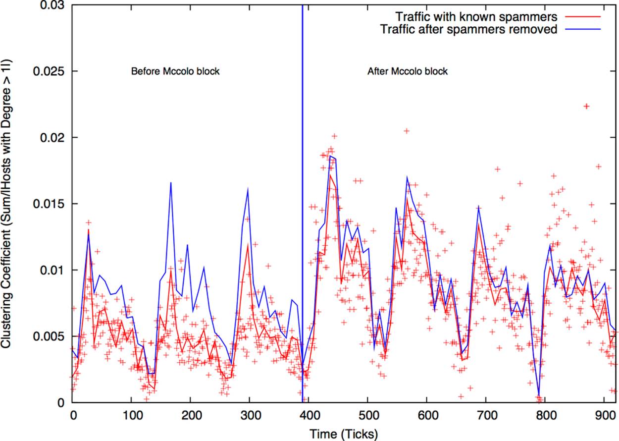
Figure 13-3. Clustering coefficient and large email networks

Analyzing Graphs

Graph analysis can be used for a number of purposes. Centrality metrics are a useful tool both for engineering and for forensic analysis, while components and graph attributes can be used to generate a number of alarms.

Using Component Analysis as an Alarm

In Chapter 11 we discussed detection mechanisms that relied on the attacker’s ignorance of a particular network, such as blind scanning and the like. Connected components are a good way of modeling a different type of attacker ignorance. An attacker might know where various servers and systems are located on a network, but he doesn’t know how they relate to each other. Organizational structure can be identified by looking at connected components, and a number of attacks such as APT and hit-list attacks, which may know the target but not how targets relate to each other, can be identified by examining these components.

To understand how this phenomenon can be used as an alarm, consider the graphical example in Figure 13-4. In this example, a network is composed of two discrete components (say, engineering and marketing), and there is little interaction between them. When an attacker appears and tries to communicate with the hosts on the network, he combines these two components to produce one huge component that does not appear under normal circumstances.

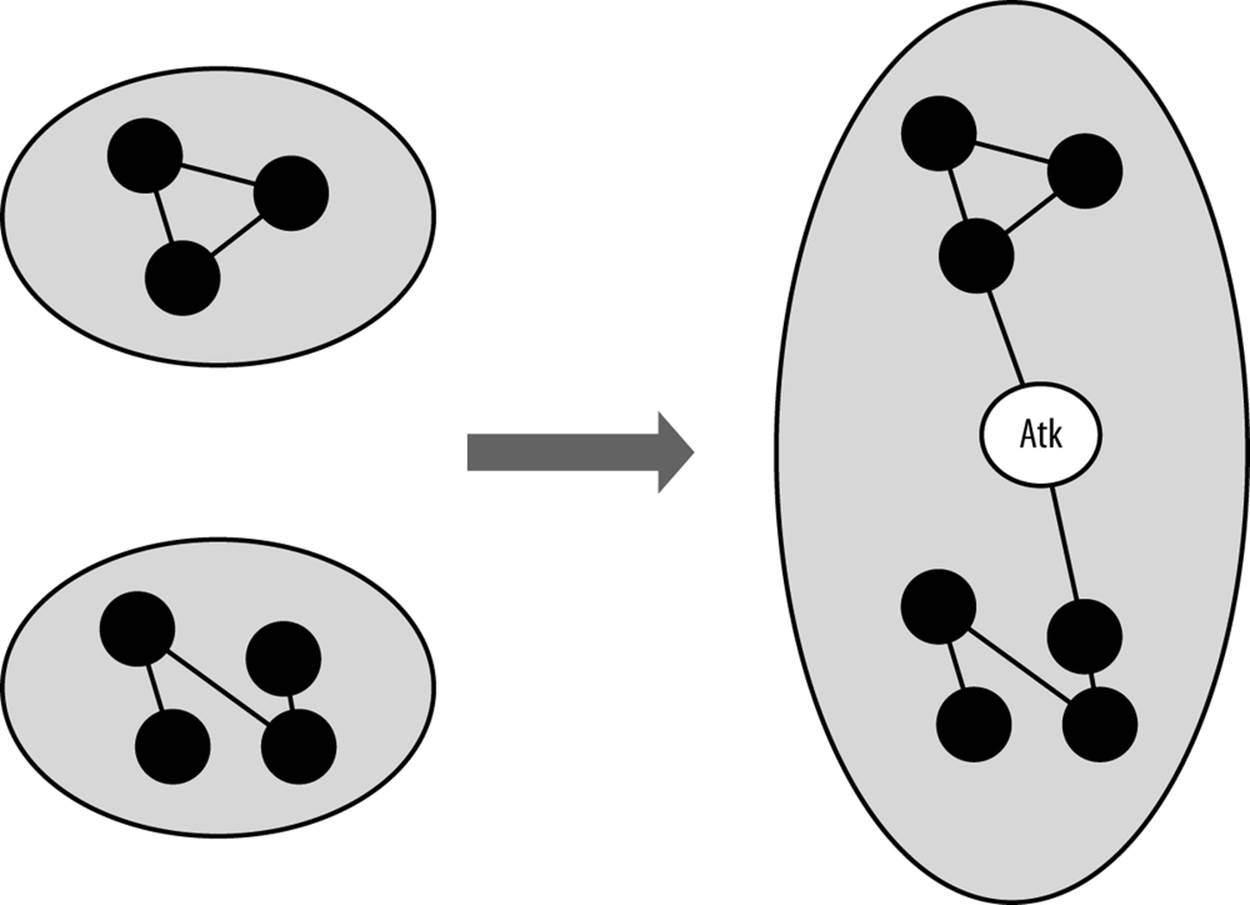
Figure 13-4. An attacker artifically links discrete components

To implement this type of alarm, you must first identify a service that can be divided into multiple components. Good candidates are services such as SSH that require some form of user login; permissions mean that certain users won’t have access, which breaks the network into discrete components. SMTP and HTTP are generally bad candidates, though HTTP is feasible if you are looking exclusively at servers that require user login, and you limit your analysis to just those servers (e.g., by using an IPSet).

After you’ve identified your set of servers, identify components to monitor. And after you identify a component, calculate its size—the number of nodes within the component as a function of the time taken to collect it (for example, 60 seconds of netflow). The distribution is likely to be sensitive not only to the time taken to collect the traffic, but also the time of day. Breaking traffic at least into on/off periods (as discussed in Chapter 12) is likely to help.

There are two ways to identify components: either by size order or by tracking hosts within the components. In the case of size order, you simply track the size of the largest component, the second largest component, and so on. This approach is simple, robust, and relatively insensitive to subtle attacks. It’s not uncommon for the largest component to make up more than one-third of the total nodes in the graph, so you need a fairly aggressive attack to disrupt the size of the component. The alternative approach involves identifying nodes by their component (e.g., component A is the component containing address 127.0.1.2).

Using Centrality Analysis for Forensics

Centrality is a useful tool for identifying important nodes in a network, and for identifying nodes that communicate at much lower volumes than traffic analysis can identify.

Consider an attack where the attacker infects one or more hosts on a network with malware. These infected hosts now communicate with a command and control server that was previously not present. Figure 13-5 shows this scenario in more depth; before hosts A, B, and C are infected, one node shows some degree of centrality. Following infection, a new node (Mal) is the most central node in the set.

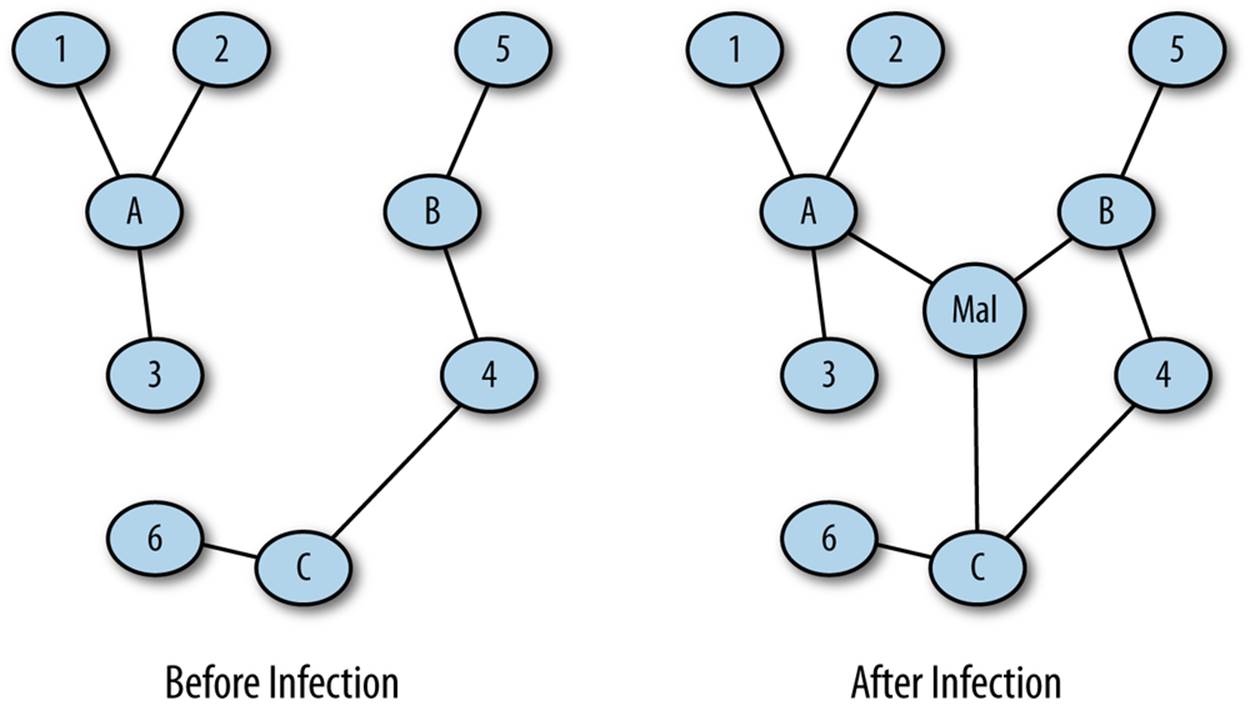
Figure 13-5. Centrality in forensics

This kind of analysis can be done by isolating traffic data into two sets, a pre-event set and a post-event set. For example, after finding out that the network received a malicious attachment at a particular time, I can pull traffic before that time to produce a pre-event set and traffic after that time to find a post-event set. Looking for newly central nodes gives me a reasonable chance of identifying the command and control server.

Using Breadth-First Searches Forensically

Once you’ve identified that a malicious host is communicating on your network, the next step is to find out who he’s talking to, such as the host’s C&C or other infected hosts on the network. Once you’ve found that out, you can repeat the process to find out who they talked to in order to identify other targets.

This iterative investigation is a breadth-first search. You start with a single node, look at all of its neighbors for suspicious behavior, and then repeat the process on their neighbors (see Example 13-6). This type of graph-based investigation can help identify other infected hosts, suspicious targets, and other systems on the network that need investigation or analysis.

Example 13-6. Examining a site’s neighbors

#!/usr/bin/env python

#

# This is a somewhat ginned-up example of how to use breadth-first searches to

# crawl through a dataset and identify other hosts that are using BitTorrent.

# The crawling criteria are as follows:

# A communicates to B on ports 6881-6889

# A and B send a large file between each other (> 1 MB)

#

# The point of the example is that you could use any criteria you want and put

# multiple criteria into constructing the graph.

#

#

# Comand line

#

# crawler.py seed_ip datafile

#

# seed_ip is the ip address of a known bittorrent user

# datafile

import os, sys, basic_graph

def extract_neighbors(ip_address, datafile):

# Given an ip_address, identify the nodes adjacent to that

# address by finding flows that have that address as either a source or

# destination. The other address in the pair is considered a neighbor.

a = os.popen("""rwfilter --any-address=%s --sport=1024-65535 --dport=1024-65535 \

--bytes=1000000- --pass=stdout %s | rwfilter --input=stdin --aport=6881-6889 \

--pass=stdout | rwuniq --fields=1,2 --no-title""" % (ip_address,datafile), 'r')

# In the query, note the fairly rigorous port definitions I'm using -- everything

# starts out as high. This is because, depending on the stack implementation,

# ports 6881-6889 (the BT ports) may be used as ephemeral ports. By breaking

# out client ports in the initial filtering call, I'm guaranteeing that I

# don't accidently record, say, a web session to port 6881.

# The 1 MB limit is also supposed to constrain us to actual BT file transfers.

neighbor_set = set()

for i in a.readlines():

sip, dip = i.split('|')[0:2].strip()

# I check to see if IP address is the source or destination of the

# flow; whichever one it is, I add the complementary address to the

# neighbor set (e.g., if ip_address is sip, I add the dip)

if sip == ip_address:

neighbor_set.add(dip)

else:

neighbor_set.add(sip)

a.close()

return neighbor_set

if __name__ == '__main__':

starting_ip = sys.argv[1]

datafile = sys.argv[2]

candidate_set = set([starting_ip])

while len(candidate_set) > 0:

target_ip = candidate_set.pop()

target_set.add(target_ip)

neighbor_set = extract_neighbors(target_ip, datafile)

for i in neighbor_set:

if not i in target_set:

candidate_set.add(i)

for i in target_set:

print i

Using Centrality Analysis for Engineering

Given limited monitoring resources and analyst attention, effectively monitoring a network requires identifying mission-critical hosts and assigning resources to protecting and watching them. That said, in any network, there’s a huge difference between the hosts that people say they need and the hosts they actually use. Using traffic analysis to identify critical hosts helps differentiate between what’s important on paper and what users actually visit.

Centrality is one of a number of metrics that can be used to identify criticality. Alternatives include counting the number of hosts that visit a site (which is effectively degree centrality) and looking at traffic volume. Centrality is a good complement to volume.

Further Reading

1. Michael Collins and Michael Reiter, “Hit-list Worm Detection and Bot Identification in Large Networks Using Protocol Graphs,” Proceedings of the 2007 Symposium on Recent Advances in Intrusion Detection.

2. Thomas Cormen, Charles Leiserson, Ronald Rivest, and Clifford Stein, Introduction to Algorithims, Third Edition (MIT Press, 2009).

3. igraph (R graph library)

4. Lun Li, David Alderson, Reiko Tanaka, John C. Doyle, and Walter Willinger, “Towards a Theory of Scale-Free Graphs: Definition, Properties, and Implications (Extended Version).”

5. Neo4j

6. Networkx (Python graph library)