Network Security Through Data Analysis: Building Situational Awareness (2014)

Part III. Analytics

Chapter 12. Volume and Time Analysis

In this chapter, we look at phenomena that can be identified by comparing traffic volume against the passage of time. “Volume” may be a simple count of the number of bytes or packets, or it may be a construct such as the number of IP addresses transferring files. Based on the traffic observed, there are a number of different phenomena that can be pulled out of traffic data, particularly:

Beaconing

When someone contacts your host at regular intervals, it is a possible sign of an attack.

File extraction

Massive downloads are suggestive of someone stealing your internal data.

Denial of Service (DoS)

Preventing your servers from providing service.

Traffic volume data is noisy. Most of the observables that you can directly count, such as the number of bytes over time, vary highly and have no real relationship between the volume of the event and its significance. In other words, there’s rarely a significant relationship between the number of bytes and the importance of the events. This chapter will help you find unusual behaviors through scripts and visualizations, but a certain amount of human eyeballing and judgment are necessary to determine which behaviors to consider dangerous.

The Workday and Its Impact on Network Traffic Volume

The bulk of traffic on an enterprise network comes from people who are paid to work there, so their traffic is going to roughly follow the hours of the business day. Traffic will trough during the evening, rise around 0800, peak around 1300, and drop off around 1800.

To show how dominant the workday is, consider Figure 12-1, a plot showing the progression of the SoBIG.F email worm across the SWITCH network in 2003. SWITCH is Switzerland and Lichtenstein’s educational network, and makes up a significant fraction of the national traffic for Switzerland. In Figure 12-1, the plot shows the total volume of SMTP traffic over time for a two-week period. SoBIG propagates at the end of the plot. But what I want to highlight is the normal activity during the earlier part of the week on the left. Note that each weekday is a notched peak, with the notch coming at lunchtime. Note also that there is considerably less activity over the weekend.

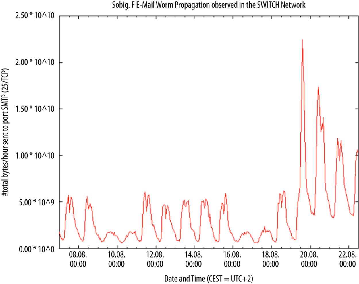
Figure 12-1. Mail traffic and propagation of a worm across Switzerland’s SWITCH network (image courtesy of Dr. Arno Wagner)

This is a social phenomenon; knowing roughly where the address you’re monitoring is (home, work, school), and the local time zone can help predict both events and volumes. For example, in the evening, streaming video companies become a more significant fraction of traffic as people kick back and watch TV.

There are a number of useful rules of thumb for working with workday schedules to identify, map, and manage anomalies. These include tracking active and inactive periods, tracking the internal schedule of an organization, and keeping track of the time zone. The techniques covered in this section are a basic, empirical approach to time series analysis; considerably more advanced techniques are covered in the books cited.

When working with site data, I usually find that it’s best to break traffic into “on” (people are working) and “off” (people are at home) periods. The histogram in Figure 12-2 shows how this phenomenon can affect the distribution of traffic volume—in this case, the two distinct peaks correspond to the on-periods and off-periods. Modeling the two periods separately will provide a more accurate volume estimate without pulling out the heavier math used for time series analysis.

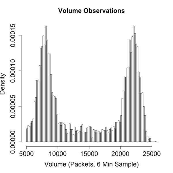
Figure 12-2. Distribution of traffic in a sample network, where the peak on the right is workday and the peak on the left is evening

When determining on-periods and off-periods, consider the schedule of the organization itself. If your company has any special or unusual holidays, such as taking a founder’s birthday off, keep track of those as potential off-days. Similarly, are there parts of the organization that are staffed constantly and other parts that are only 9 to 5? If something is constantly staffed, keep track of the shift changes, and you’ll often see traffic repeat at the start of a shift as everyone logs on, checks email, meets, and then starts working.

THE VALUE OF OFF-DAYS

Off-time is valuable. If I want to identify dial-homes, file exfiltration, and other suspicious activity, I like to do so by watching off-hours. There’s less traffic, there are fewer people, and if someone is ignorant of a company’s internal circadian rhythm, she’ll be a lot easier to identify during those periods than if she’s hiding in the crowd.

This is the reason I like to keep track of a company’s own special off-times. It’s easy enough for someone to hide his traffic by keeping all activity in 9–5/M–F, but if the attacker doesn’t know the company gives St. Swithin’s Day off, then he’s more likely to stick out.

I’ve seen this particular phenomenon show up when dealing with insiders, particularly people worried about shoulder surfing or physical surveillance. They’ll move their activity to evenings and weekends in order to make sure their neighbors don’t ask what they’re doing, and then show up fairly visibly in the traffic logs.

Business processes are a common source of false positives with volume analysis. For example, I’ve seen a corporate site where there’s a sudden biweekly spike in traffic to a particular server. The server, which covered company payroll, was checked by every employee every other Friday and never visited otherwise. Phenomena that occurs weekly, biweekly, or on multiples of 30 days is likely to be associated with the business’s own processes and should be identified as such for future reference.

Beaconing

Beaconing is the process of systematically and regularly contacting a host. For instance, botnets will poll their command servers for new instructions periodically. This is particularly true of many modern botnets that use HTTP as a moderator. Such behavior will appear to you as information flows at regular intervals between infected systems on your site and an unknown address off-site.

However, there are many legitimate behaviors that also generate routine traffic flows. Examples include:

Keep alives

Long-lived sessions, such as an interactive SSH session, will send empty packets at regular intervals in order to maintain a connection with the target.

Software updates

Most modern applications include some form of automated update checkup. AV, in particular, regularly downloads signature updates to keep track of the latest malware.

News and weather

Many news, weather, and other interactive sites regularly refresh the page as long as a client is open to read it.

Beacon detection is a two-stage process. The first stage involves identifying consistent signals. An example process for doing so is the find_beacons.py script shown in Example 12-1. find_beacons.py takes a sequence of flow records and dumps them into equally sized bins. Each input consists of two fields: the IP address where an event was found and the starting time of the flow, as returned by rwcut. rwsort is used to order the traffic by source IP and time.

The script then checks the median distance between the bins and scores each IP address on the fraction of bins that fall within some tolerance of that median. If a large number of flows are near the median, you have found a regularly recurring event.

Example 12-1. A simple beacon detector

#!/usr/bin/env python

#

#

# find_beacons.py

#

# input:

# rwsort --field=1,9 | rwcut --no-title --epoch --field=1,9 | <stdin>

# command line:

# find_beacons.py precision tolerance [epoch]

#

# precision: integer expression for bin size (in seconds)

# tolerance: floating point representation for tolerance expressed as

# fraction from median, e.g. 0.05 means anything within (median -

# 0.5*median, median + 0.5*median) is acceptable

# epoch: starting time for bins; if not specified, set to midnight of the first

# time read.

# This is a very simple beacon detection script which works by breaking a traffic

# feed into [precision] length bins. The distance between bins is calculated and

# the median value is used as representative of the distance. If all the distances

# are within tolerance% of the median value, the traffic is treated as a beacon.

import sys

if len(sys.argv) >= 3:

precision = int(sys.argv[1])

tolerance = float(sys.argv[2])

else:

sys.stderr.write("Specify the precision and tolerance\n")

starting_epoch = -1

if len(sys.argv) >= 4:

starting_epoch = int(sys.argv[3])

current_ip = ''

def process_epoch_info(bins):

a = bins.keys()

a.sort()

distances = []

# We create a table of distances between the bins

for i in range(0, len(a) -1):

distances.append(a[i + 1] - a[i])

distances.sort()

median = distances(len(distances)/2)

tolerance_range = (median - tolerance * median, median + tolerance *median)

# Now we check bins

count = 0

for i in distances:

if (i >= tolerance_range[0]) and (i <= tolerance_range[1]):

count+=1

return count, len(distances)

bins = {} # Checklist of bins hit during construction; sorted and

# compared later. AA be cause it's really a set and I

# should start using those.

results = {} # Associate array containing the results of the binning

# analysis, dumped during the final report

# We start reading in data; for each line I'm building a table of

# beaconing events. The beaconing events are simply indications that

# traffic 'occurred' at time X. The size of the traffic, how often it occurred,

# how many flows is irrelevant. Something happened, or it didnt.

for i in sys.stdin.readlines():

ip, time = i.split('|')[0:2]

if ip != current_ip:

results[ip] = process_epoch_info(bins)

bins = {}

if starting_epoch == -1:

starting_epoch = time - (time % 86400) # Sets it to midnight of that day

bin = (time - starting_epoch) / precision

bins[bin] = 1

a = bins.sort()

for i in a:

print "%15s|%5d|%5d|%8.4f" % (ip, bins[a][0], bins[a][1],

100.0 * (float(bins[a[0]])/float(bins[a[1]])))

The second stage of beacon detection (as usual) is inventory management. An enormous number of legitimate applications, as we saw earlier, transmit data periodically. NTP, routing protocols, and AV tools all dial home on a regular basis for information updates. SSH also tends to show periodic behavior, because administrators run periodic maintenance tasks via the protocol.

File Transfers/Raiding

Data theft is still the most basic form of attack on a database or website, especially if the website is internal or an otherwise protected resource. For lack of a better term, I’ll use raiding to denote copying a website or database in order to later disseminate, dump, or sell the information. The difference between raiding and legitimate access is a matter of degree, as the point of any server is to serve data.

Obviously, raiding should result in a change in traffic volume. Raiding is usually conducted quickly (possibly while someone is packing up her cubicle) and often relies on automated tools such as wget. It’s possible to subtly raid, but that would require the attacker to have both the time to slowly extract data and the patience to do so.

Volume is one of the easiest ways to identify a raid. The first step is building up a model of the normal volume originating from a host over time. The calibrate_raid.py script in Example 12-2 provides thresholds for volume over time, as well as a table of results to plot.

Example 12-2. A raid detection script

#!/usr/bin/env python

#

# calibrate_raid.py

#

# input:

# Nothing

# output:

# writes a report containing a time series and volume estimates to stdout

# command_line

# calibrate_raid.py start_date end_date ip_address server_port period_size

#

# start_date: The date to begin the query on

# end_date: The date to end the query on

# ip_address: the server address to query

# server_port: the port of the server to query

# period_size: the size of the periods to use for modeling the time

#

# Given a particular IP address, this generates a time series (via rwcount)

# and a breakdown on what the expected values at the 90-100% thresholds would

# be. The count output can then be run through a visualizer in order to

# check for outliers or anomalies.

#

import sys,os,tempfile

start_date = sys.argv[1]

end_date = sys.argv[2]

ip_address = sys.argv[3]

server_port = int(sys.argv[4])

period_size = int(size.arg[5])

if __name__ == '__main__':

fh, temp_countfn = tempfile.mkstemp()

os.close(fh)

# Note that the filter call uses the IP address as the source, and the

# server port as the source. We're pulling out flows that originated

# FROM the server, which means that they should be the data from the

# file transfer. If we used daddress/dport, we'd be logging the

# (much smaller) requests to the server from the clients.

#

os.system(('rwfilter --saddress=%s --sport=%d --start-date=%s ',

'--end-date=%s --pass=stdout | rwcount --epoch-slots',

' --bin-size=%d --no-title > %s') % (

ip_address, server_port, start_date, end_date, period_size,

temp_countfn))

# A note on the filtering I'm doing here. You *could* rwfilter to

# only include 4-packet or above sessions, therefore avoiding the

# scan responses. However, those *should* be minuscule, and

# therefore I elect not to in this case.

# Load the count file into memory and add some structure

#

a = open(temp_countfn, 'r')

# We're basically just throwing everything into a histogram, so I need

# to establish a min and max

min = 99999999999L

max = -1

data = {}

for i in a.readlines():

time, records, bytes, packets = map(lambda x:float(x),

i[:-1].split('|')[0:4])

if bytes < min:

min = bytes

if bytes > max:

max = bytes

data[time] = (records, bytes, packets)

a.close()

os.unlink(temp_countfn)

# Build a histogram with hist_size slots

histogram = []

hist_size = 100

for i in range(0,hist_size):

histogram.append(0)

bin_size = (max - min) / hist_size

total_entries = len(data.values)

for records, bytes, packets in data.values():

bin_index = (bytes - min)/bin_size

histogram[bin_index] += 1

# Now we calculate the thresholds from 90 to 100%

thresholds = []

for i in range(90, 100):

thresholds.append(0.01 * i * total_entries)

total = 0

last_match = 0 # index in thresholds where we stopped

# Step 1, we dump the thresholds

for i in range(0, hist_size):

total += histogram[i]

if total >= thresholds[last_match]:

while thresholds[last_match] < total:

print "%3d%% | %d" % (90 + last_match, (i * bin_size) + min)

a = data.keys()

a.sort()

for i in a:

print "%15d|%10d|%10d|%10d" % (i, data[i][0], data[i][1], data[i][2])

Visualization is critical when calibrating volume thresholds for detecting raiding or other raiding anomalies. We’ve discussed the problem with standard deviations in Chapter 10, and a histogram is the easiest way to determine whether a distribution is even remotely Gaussian. In my experience, a surprising number of services regularly raid hosts—web spiders and the Internet archive being among the more notable examples. If a site is strictly internal, backups and internal mirroring are common false positives.

Visualization can identify these outliers. The example in Figure 12-3 shows that the overwhelming majority of traffic occurs below about 1000 MB/10 min, but those few outliers above 2000 MB/10 min will cause problems for calibrate_raid.py and most training algorithms. Once you have identified the outliers, you can record them in a whitelist and remove them from the filter command using --not-dipset. You can then use rwcount to set up a simple alert mechanism.

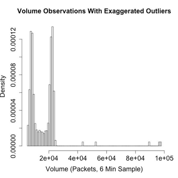
Figure 12-3. Traffic volume with outliers; determining the origin and cause of outliers will reduce alerts

Locality

Locality is the tendency of references (memory locations, URLs, IP addresses) to cluster together. For example, if you track the web pages visited by a user over time, you will find that the majority of pages are located in a small and predictable number of sites (spatial locality), and that users tend to visit the same number of sites over and over (temporal locality). Locality is a well understood concept in computer science, and serves as the foundation of caching, CDNs, and reverse proxies.

Locality is particularly useful as a complement to volumetric analysis because users are generally predictable. Users visit a small number of sites and talk to a small number of people, and while there are occasional changes, we can model this behavior using a working set.

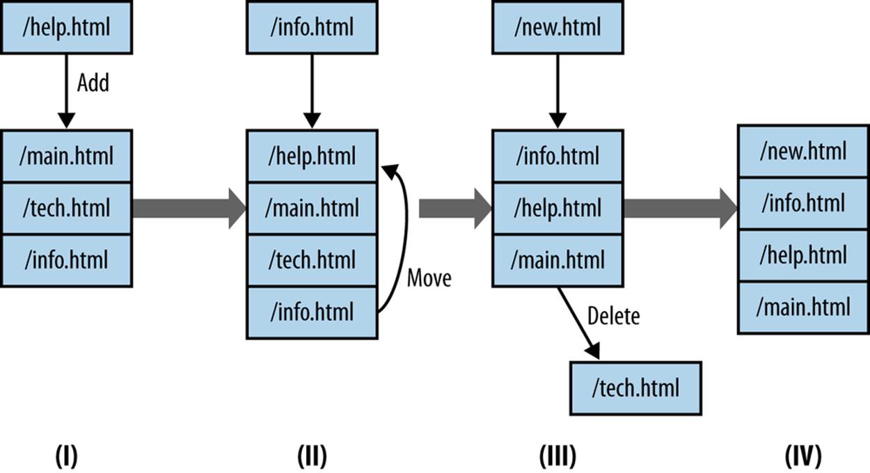
Figure 12-4. A Working Set in Operation

Figure 12-4 is a graphical example of a working set in operation. In this example, the working set is implemented as an LRU (Least Recently Used) queue of fixed size (in this case, four references in the queue). This working set is tracking web surfing, so it gets fed URLs from an HTTP server logfile and adds them to the stack. Working sets only keep one copy of every reference they see, so a four-reference set like the one shown in Figure 12-4 will only show four references. When a working set receives a reference, it does one of three things:

1. If there are empty references left, the new reference is enqueued at the back of the queue (I to II).

2. If the queue is filled AND the reference is present, the reference is moved to the back of the queue.

3. If the queue is filled AND the reference is NOT present, then the reference is enqueued at the back of the queue, and the reference at the front of the queue is removed.

The code in Example 12-3 shows an LRU working set model in python.

Example 12-3. Calculating working set characteristics

#!/usr/bin/env python

#

#

# Describe the locality of a host using working_set depth analysis.

# Inputs:

# stdin - a sequence of tags

#

# Command line args:

# first: working_set depth

import sys

try:

working_set_depth = int(sys.argv[1])

except:

sys.stderr.write("Specify a working_set depth at the command line\n")

sys.exit(-1)

working_set = []

i = sys.stdin.readline()

total_processed = 0

total_popped = 0

unique_symbols = {}

while i != '':

value = i[:-1] #Ditch the obligatory \n

unique_symbols[value] = 1 # Add in the symbol

total_processed += 1

try:

vind = working_set.index(value)

except:

vind = -1

if (vind == -1):

# Value isn't present as an LRU cache; delete the

# least recently used value and store this at the end

working_set.append(value)

if len(working_set) > working_set_depth:

del working_set[0]

working_set.append(value)

total_popped +=1

else:

# Most recently used value; move it to the end of the working_set

del working_set[vind]

# Calculate probability of replacement stat

p_replace = 100.0 * (float(total_popped)/float(total_processed))

print "%10d %10d %10d %8.4f" % (total_processed, unique_symbols,

working_set_depth, p_replace)

Figure 12-5 shows an example of what working sets will look like. This figure plots the probability of replacing a value in the working set as a function of the working set size. Two different sets are compared here: a completely random set where references are picked from a set of 10 million symbols, and a model of user activity using a Pareto distribution. The Pareto model is adequate for modeling normal user activity, if actually a bit less stable than users under normal circumstances.

Note the “knee” in the Pareto model, while the random model remains consistent at a 100% replacement rate. Working sets generally have an ideal size after which increasing the set’s size is counterproductive. This knee is representative of this phenomenon—you can see that the probability of replacement drops slightly before the knee, but remains effectively stable afterward.

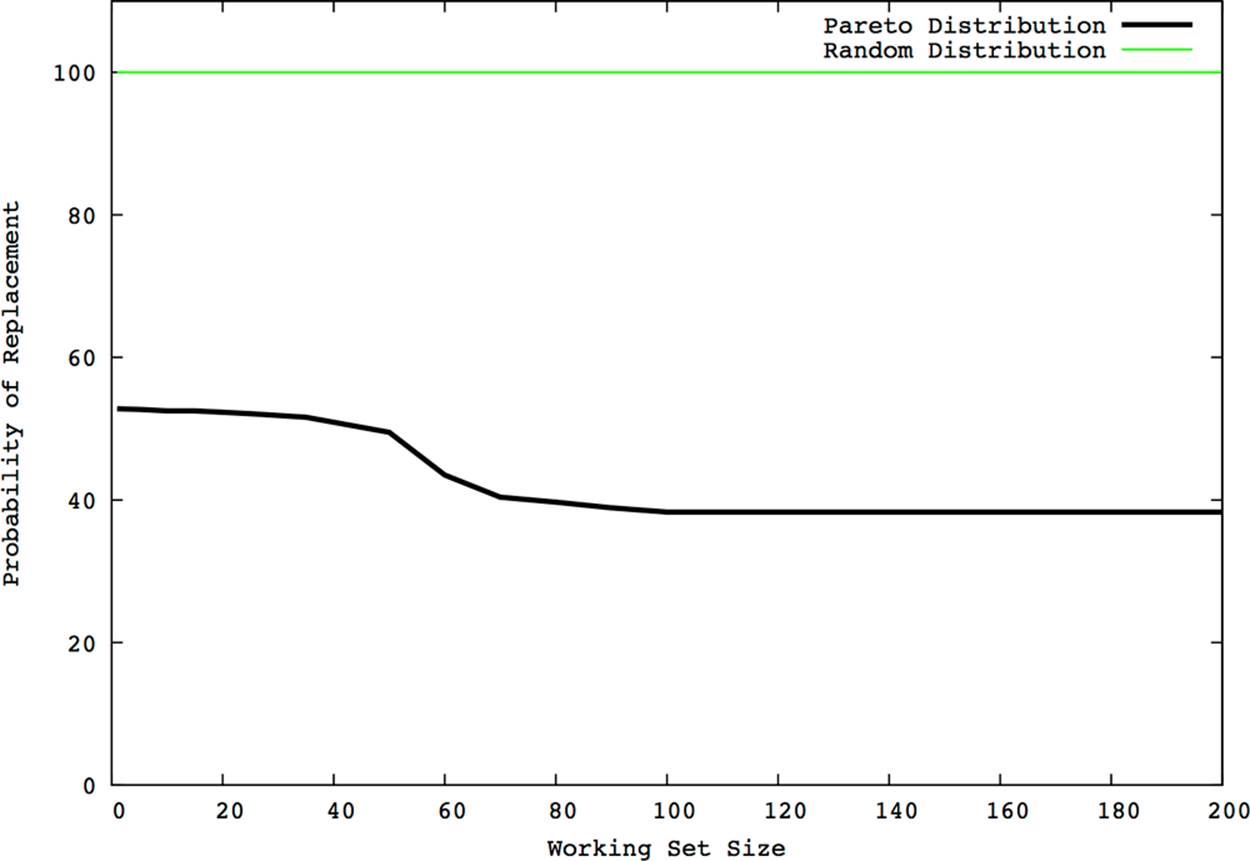
Figure 12-5. Working set analysis

The value of working sets is that once they’re calibrated, they reduce user habit down to two parameters: the size of the queue modeling the set and the probability that a reference will result in a queue replacement.

DDoS, Flash Crowds, and Resource Exhaustion

Denial of Service (DoS) is a goal, not a specific strategy. A DoS results in a host that cannot be reached from remote locations. Most DoS attacks are implemented as a Distributed Denial of Service (DDoS) attack in which the attacker uses a network of captured hosts in order to implement the DoS. There are several ways an attacker can implement DoS, including but not limited to:

Service level exhaustion

The targeted host runs a publicly accessible service. Using a botnet, the attacker starts a set of clients on the target, each conducting some trivial but service-specific interaction (such as fetching the home page of a website).

SYN flood

The SYN flood is the classic DDoS attack. Given a target with an open TCP port, the attacker sends clients against the attacker. The clients don’t use the service on the port, but simply open connections using a SYN packet and leave the connection open.

Bandwidth exhaustion

Instead of targeting a host, the attacker sends a massive flood of garbage traffic towards the host, intending to overwhelm the connection between the router and the target.

And you shouldn’t ignore a simple insider attack: the attacker walks over to the physical server and disconnects it.

All these tactics produce the same result, but each tactic will appear differently in network traffic and may require different mitigation techniques. Exactly how many resources the attacker needs is a function of how the attacker implements DDoS. As a rule of thumb, the higher up an attack is on the OSI model, the more stress it places on the target and the fewer bots are required by the attacker. For example, bandwidth exhaustion hits the router and basically has to exhaust the router interface. SYN flooding, the classic DDoS attack, has to simply exhaust the target’s TCP stack. At higher levels, tools like Slowloris effectively create a partial HTTP connection, exhausting the resources of the web server.

This has several advantages from an attacker’s perspective. Fewer resources consumed means fewer bots involved and a legitimate session is more likely to be allowed through by a firewall that might block a packet crafted to attack the IP or TCP layer.

DDoS and Routing Infrastructure

DDoS attacks aimed specifically at routing infrastructure will produce collateral damage. Consider a simple network like the one in Figure 12-6; the heavy line shows the path of the attack to subnetwork C. The attacker hitting subnetwork C is exhausting not just the connection at C, but also the router’s connection to the Internet. Consequently, hosts on networks A and B will not be able to reach the Internet and will see their incoming Internet traffic effectively drop to zero.

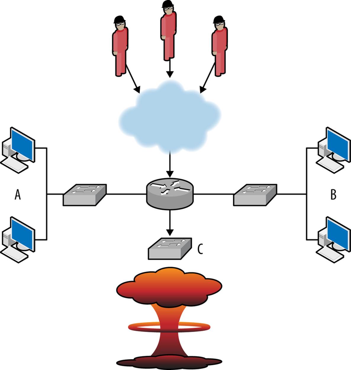
Figure 12-6. DDoS collateral damage

This type of problem is not uncommon on colocated services, and emphasizes that DDoS defense is rooted at network infrastructure. I am, in the long run, deeply curious to see how cloud computing and DDoS are going to marry. Cloud computing enables defenders to run highly distributed services across the Internet’s routing infrastructure. This, in turn, increases the resources the attacker needs to take out a single defender.

With DoS attacks, the most common false positives are flash crowds and cable cuts. A flash crowd is a sudden influx of legitimate traffic to a site in response to some kind of announcement or notification. Alternate names for flash crowds such as SlashDot effect, farking, or Reddit effectprovide a good explanation of what’s going on.

These different classes of attacks are usually easily distinguished by looking at a graph of incoming traffic. Some idealized images are shown in Figure 12-7, which explain the basic phenomena.

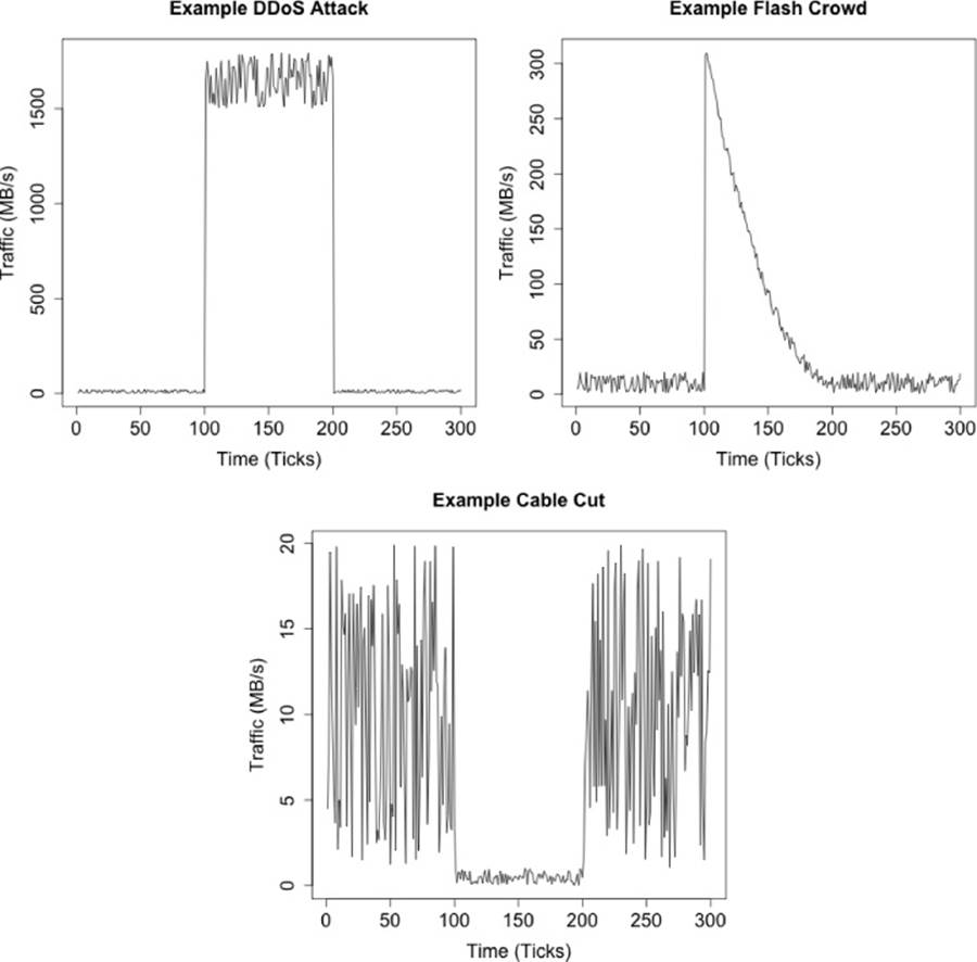
Figure 12-7. Different classes of bandwidth exhaustion

The images in Figure 12-7 describe three different classes of bandwidth exhaustion: a DDoS, a flash crowd, and a cable cut or other infrastructure failure. Each plot is of incoming traffic and equivalent to sitting right at the sensor. The differences between the plots reflect the phenomena causing the problems.

DDoS attacks are mechanical. The attack usually switches on and off instantly, as the attacker is issuing commands remotely to a network of bots. When a DDoS starts, it almost instantly consumes as much bandwidth as available. In many DDoS plots, the upper limit on the plot is dictated by the networking infrastructure: if you have a 10 GB pipe, the plot maxes at 10 GB. DDoS attacks are also consistent. Once they start, they generally keep humming along at about the same volume. Most of the time, the attacker has grossly overprovisioned the attack. Bots are being removed while the attack goes on, but there’s more than enough to consume all available bandwidth even if a significant fraction are knocked offline.

DDoS mitigation is an endurance contest. The best defense is to provision out bandwidth before the attack starts. Once an attack actually occurs, the best you can do at any particular location is to try to identify patterns in the traffic and block the ones causing the most damage. Examples of patterns to look for include:

§ Identifying a core audience for the target and limiting traffic to the core audience. The audience may be identified by using IP address, netblock, country code, or language, among other attributes. What is critical is that the audience has a limited overlap with the attacker set. The script inExample 12-4 provides a mechanism for ordering /24s by the difference between two sets: historical users that you trust and new users whom you suspect of being part of a DDoS attack.

§ Spoofed attacks are occasionally identifiable by some flaw in the spoofing. The random number generator for the spoof might set all addresses to x.x.x.1, as an example.

Example 12-4. An example script for ordering blocks

#!/usr/bin/env python

#

# ddos_intersection.py

#

# input:

# Nothing

# output:

# A report comparing the number of addresses in two sets, ordered by the

# largest number of hosts in set A which are not present in set B.

#

# command_line

# ddos_intersection.py historical_set ddos_set

#

# historical_set: a set of historical data giving external addresses

# which have historically spoken to a particular host or network

# ddos_set: a set of data from a ddos attack on the host

# This is going to work off of /24's for simplicity.

#

import sys,os,tempfile

historical_setfn = sys.argv[1]

ddos_setfn = sys.argv[2]

blocksize = int(sys.argv[3])

mask_fh, mask_fn = tempfile.mkstemp()

os.close(mask_fh)

os.unlink(mask_fn)

os.system(('rwsettool --mask=24 --output-path=stdout %s | ' +

' rwsetcat | sed 's/$/\/24/' | rwsetbuild stdin %s') %

(historical_setfn, mask_fn))

bins = {}

# Read and store all the /24's in the historical data

a = os.popen(('rwsettool --difference %s %s --output-path=stdout | ',

'rwsetcat --network-structure=C') % (mask_fn, historical_setfn),'r')

# First column is historical, second column is ddos

for i in a.readlines():

address, count = i[:-1].split('|')[0:2]

bins[address] = [int(count), 0]

a.close()

# Repeat the process with all the data in the ddos set

a = os.popen(('rwsettool --difference %s %s --output-path=stdout | ',

'rwsetcat --network-structure=C') % (mask_fn, ddos_setfn),'r')

for i in a.readlines():

address, count = i[:-1].split('|')[0:2]

# I'm intersecting the maskfile again, since I originally intersected it against

# the file I generated the maskfile from, any address that I find in the file

# will already be in the bins associative array

bins[address][1] = int(count)

#

# Now we order the contents of the bins. This script is implicitly written to

# support a whitelist-based approach -- addresses which appear in the historical

# data are candidates for whitelisting, all other addresses will be blocked.

# We order the candidate blocks in terms of the number of historical addresses

# allowed in, decreasing for every attacker address allowed in.

address_list = bins.items()

address_list.sort(lambda x,y:(y[1][0]-x[1][0])-(y[1][1]-x[1][1]))

print "%20s|%10s|%10s" % ("Block", "Not-DDoS", "DDoS")

for address, result in address_list:

print "%20s|%10d|%10d" % (address, bins[address][0], bins[address][1])

This type of filtering works more effectively if the attack is focused on striking a specific service, such as DDoSing a web server with HTTP requests. If the attacker is instead focused on traffic flooding a router interface, the best defenses will normally lie upstream from you.

As discussed in Chapter 11, people are impatient where machines are not, and this behavior is the easiest way to differentiate flash crowds from DDoS attacks. As the flash crowd plot in Figure 12-7 shows, when the event occurs, the initial burst of bandwidth is followed by a rapid falloff. The falloff is because people have discovered that they can’t reach the targeted site and have moved on to more interesting pastures until some later time.

Flash crowds are public affairs—for some reason, somebody publicized the target. As a result, it’s often possible to figure out the origin of the flash crowd. For example, HTTP referrer logs will include a reference to the site. Googling the targeted site is often a good option. If you are familiar with the press and news associated with your site, this is also a good option.

Cable cuts and mechanical failures will result in an actual drop in traffic. This is shown in the cable cut figure, where all of a sudden traffic goes to zero. When this happens, the first follow-up step is to try to generate some traffic to the target, and ensure that the problem is actually a failure in traffic and not a failure in the detector. After that, you need to bring an alternate system online and then research the cause of the failure.

DDOS AND FORCE MULTIPLIERS

Functionally, DDoSes are wars of attrition: how much traffic can the attacker throw at the target, and how can the target compensate for that bandwidth? Attackers can improve the impact of their attack through a couple of different strategies: they can acquire more resources, attack at different layers of the stack, and rely on Internet infrastructure to inflict additional damage. Each of these techniques effectively serves as a force multiplier for attackers, increasing the havoc with the same number of bots under their control.

The process of resource acquisition is really up to the attacker. The modern Internet underground provides a mature market for the rental and use of botnets. An alternative approach, used notably by some of Anonymous, involves volunteers. Anonymous has developed a family of JavaScript and C# DDoS tools under the monicker “LOIC” (Low Orbit Ion Cannon) to conduct DDoS attacks. The LOIC family of tools are, in comparison to hardcore malware, fairly primitive. Arguably, they’re not intended to be anything more than that given their hacktivist audience.

These techniques rely on processing asymmetry: the attacker in some way juggles operations so that the processing demand on the server per connection is higher than the processing demand on the client. Development decisions will impact a system’s vulnerability to a higher-level DDoS.^[24^]

Attackers can also rely on Internet infrastructure to conduct attacks. This is generally done by taking a response service and sending the response to a forged target address. The classic example of this, the smurf attack, consisted of a ping where the host A, wanting to DDoS site B, sends a spoofed ping to a broadcast address. Every host receiving the ping (i.e., everything sharing the broadcast address) then drowns the target in responses. The most common modern form of this attack uses DNS reflection: the attacker sends a spoofed request to a DNS resolver, which then sends an inordinately informative and helpfully large packet in response.

Applying Volume and Locality Analysis

The phenomena discussed in this chapter are detectable using a number of different approaches. In general, the problem is not so much detecting them as differentiating malicious activity from legitimate but similar-appearing activity. In this section, we discuss a number of different ways to build detectors and limit false positives.

Data Selection

Traffic data is noisy, and there’s little correlation between the volume of traffic and the malice of a phenomenon. An attacker can control a network using ssh and generate much less traffic than a legitimate user sending an attachment over email. The basic noisiness of the data is further exacerbated by the presence of garbage traffic such as scanning and other background radiation (see Chapter 11 for more information on this).

The most obvious values to work with when examining volume are byte and packet counts over a period. They are also generally so fantastically noisy that you’re best off using them to identify DDoS and raiding attacks and little else.

Because the values are so noisy and so easily disrupted, I prefer working with constructed value such as a flow. NetFlow groups traffic into session approximations; I can then filter the flows on different behaviors, such as:

§ Filtering traffic that talks only to legitimate hosts and not to dark space, this approach requires access to a current map of the network, as discussed in Chapter 15.

§ Splitting short TCP sessions (four packets or less) from longer sessions, or looking for other indications that a session is legitimate, such as the presence of a PSH flag. See Chapter 11 for more discussion on this behavior.

§ Further partitioning traffic into command, fumble, and file transfers. This approach, discussed in Chapter 14, extends the filtering process to different classes of traffic, some of which should be rare.

§ Using simple volume thresholds. Instead of recording the byte count, for example, record the number of 100, 1000, 10000, and 100000+ byte flows received. This will reduce the noise you’re dealing with.

Whenever you’re doing this kind of filtering, it’s important to not simply throw out the data, but actually partition it. For example, if you count thresholded volume, record the 1–100, 100+, 1000+, 10000+ and 100000+ values as separate time series. The reason for partitioning the data is purely paranoia. Any time you introduce a hard rule for what data you’re going to ignore, you’ve created an opening for an attacker to imitate the ignored data.

A less noisy alternative to volume counts are values such as the number of IP addresses reaching a network or the number of unique URLs fetched. These values are more computationally expensive to calculate as they require distinguishing individual values; this can be done using a tool likerwset in the SiLK suite or with an associative array. Address counts are generally more stable than volume counts, but at least splitting off the hosts who are only scanning is (again) a good idea to reduce the noise.

Example 12-5 illustrates how to apply filtering and partitioning to flow data in order to produce time series data.

Example 12-5. A simple time series output application

#

#

# gen_timeseries.py

#

# Generates a timeseries output by reading flow records and partitioning

# the data in this case, into short (<=4 packet) TCP flows, and long

# (>4 packet) TCP flows.

#

# Output

# Time <bytes> <packets> <addresses> <long bytes> <long packets> <long addresses>

#

# Takes as input

# rwcut --fields=sip,dip,bytes,packets,stime --epoch-time --no-title

#

# We assume that the records are chronologically ordered, that is, no record

# will produce an stime earlier than the records preceding it in the

# output.

import sys

current_time = sys.maxint

start_time = sys.maxint

bin_size = 300 # We'll use five minute bins for convenience

ip_set_long = set()

ip_set_short = set()

byte_count_long = 0

byte_count_short = 0

packet_count_long = 0

packet_count_short = 0

for i in sys.stdin.readlines():

sip, dip, bytes, packets, stime = i[:-1].split('|')[0:5]

# convert the non integer values

bytes, packets, stime = map(lambda x: int(float(x)), (bytes, packets, stime))

# Now we check the time binning; if we're onto a new bin, dump and

# reset the contents

if (stime < current_time) or (stime > current_time + bin_size):

ip_set_long = set()

ip_set_short = set()

byte_count_long = byte_count_short = 0

packet_count_long = packet_count_short = 0

if (current_time == sys.maxint):

# Set the time to a 5 minute period at the start of the

# currently observed epoch. This is done in order to

# ensure that the time values are always some multiple

# of five minutes apart, as opposed to dumping something

# at t, t+307, t+619 and so on.

current_time = stime - (stime % bin_size)

else:

# Now we output results

print "%10d %10d %10d %10d %10d %10d %10d" % (

current_time, len(ip_set_short), byte_count_short,

packet_count_short,len(ip_set_long), byte_count_long,

packet_count_long)

current_time = stime - (stime % bin_size)

else:

# Instead of printing, we're just adding up data

# First, determine if the flow is long or short

if (packets <= 4):

# flow is short

byte_count_short += bytes

packet_count_short += packets

ip_set_short.update([sip,dip])

else:

byte_count_long += bytes

packet_count_long += packets

ip_set_long.update([sip,dip])

if byte_count_long + byte_count_short != 0:

# Final print line check

print "%10d %10d %10d %10d %10d %10d %10d" % (

current_time, len(ip_set_short), byte_count_short,

packet_count_short,len(ip_set_long), byte_count_long,

packet_count_long)

Keep track of what you’re partitioning and analyzing. For example, if you decide to calculate thresholds for a volume-based alarm only on sessions from Bulgaria that have at least 100 bytes, then you need to make sure that approach is used to calculate future thresholds, but that it’s also documented, and why.

Using Volume as an Alarm

The easiest way to construct a volume-based alarm is to calculate a histogram and then pick thresholds based on the probability that a sample will exceed the observed threshold. calibrate_raid in Example 12-2 is a good example of this kind of threshold calculation. When generating alarms, consider the time of day issues discussed in The Workday and Its Impact on Network Traffic Volume, and whether you want multiple models; a single model will normally cost you precision. Also, when considering thresholds, consider the impact of unusually low values and whether they merit investigation.

Given the noisiness of traffic volume data, expect a significant number of false positives. Most false positives for volume breaches come from hosts that have a legitimate reason for copying or archiving a target, such as a web crawler or archiving software. Several of the IDS mitigation techniques discussed in Enhancing IDS Response are useful here; in particular, whitelisting anomalies after identifying that the source is innocuous and rolling up events.

Using Beaconing as an Alarm

Beaconing is used to detect a host that is consistently communicating with other hosts. To identify malicious activity, beaconing is primarily used to identify communications with a botnet command and control server. To detect beacons, you identify hosts that communicate consistently over a time window, as done with find_beacons.py.

Beacon detection runs into an enormous number of false positives because software updates, AV updates, and even SSH cron jobs have consistent and predictable intervals. Beacon detection consequently depends heavily on inventory management. After receiving an alert, you will have to determine whether a beaconing host has a legitimate justification, which you can do if the beaconing is from a known protocol, is communicating with a legitimate host, or provides other evidence that the traffic is not botnet C&C traffic. Once identified as legitimate, the indicia of the beacon (the address and likely the port used for communication) should be recorded to prevent further false positives.

Also of import are hosts that are supposed to be beaconing, but don’t. This is particularly critical when dealing with AV software, because attackers often disable AV when converting a newly owned host. Checking to see that all the hosts that are supposed to visit an update site do so is a useful alternative alarm.

Using Locality as an Alarm

Locality measures user habits. The advantage of the working set model is that it provides room for those habits to break. Although people are predictable, they do mail new contacts or visit new websites at irregular intervals. Locality-based alarms are consequently useful for measuring changes in user habits, such as differentiating the normal user of a website from someone who is raiding it, or identifying when a site’s audience changes during a DDoS.

Locality is a useful complement to volume-based detection for identifying raiding. A host that is raiding the site or otherwise scanning it will demonstrate minimal locality, as it will want to visit all the pages on the site as quickly as possible. In order to determine whether or not a host is raiding, look at what the host is fetching and the speed at which the host is working.

The most common false positives in this case are search engines and bots such as Googlebot. A well-behaved bot can be identified by its User-Agent string, and if the host is not identified as a bot by that string, you have a dangerous host.

A working set model can also be applied to a server rather than individual users. Such a working set is going to be considerably larger than a user profile, but it is possible to use that set to track the core audience of a website or an SSH server.

Engineering Solutions

Raid detection is a good example of a scenario in which you can apply analysis and are probably better off not building a detector. The histograms generated by calibrate_raid.py or analysis done by counting the expected volume a user pulls over a day is ultimately about determining how much data a user will realistically access from a server.

This same information can be used to impose rate limits on the servers. Instead of firing off an alert when a user exceeds this threshold, use a rate limiting module (such as Apache’s Quota) to cut the user off. If you’re worried about user revolt, set the threshold to 200% of the maximum you observe and identify outliers who need special permissions to exceed even that high threshold.

This approach is going to be most effective when you’ve got a server whose data radically exceeds the average usage of any one user. If people access a server and use less than a megabyte of traffic a day, whereas the server has gigabytes of data, you’ve got an easily defensible target.

Further Reading

1. Avril Coghlan, “A Little Book of R for Time Series”

2. John McHugh and Carrie Gates, “Locality: A New Paradigm in Anomaly Detection,” Proceedings of the 2003 New Security Paradigms Workshop.