QuickBooks 2017 All-In-One For Dummies (2016)

Book 6

Business Plans

Chapter 2

Creating a Business Plan Forecast

IN THIS CHAPTER

Enjoying a little refresher on financial statements and ratios

Working with the business plan workbook

Understanding the workbook’s formulas

Customizing the workbook

Pro forma financial statements — which are income statements, balance sheets, and cash flow statements — constitute an integral part of business planning and the overall budgeting process. For that reason, I want to provide you a bit of information about how you create such pro forma (or as if) statements.

From the very start, however, I need to warn you that to create such statements, you need a tool in addition to QuickBooks. Specifically, you need a spreadsheet program such as Microsoft Excel.

Assuming that you do have something like Excel, you can use it and the example workbook that this chapter describes to create a simple, yet sophisticated, financial forecast for your business. To download the workbook, just type http://stephenlnelson.com/wp-content/uploads/10_year_bizplan-1.xlsx in your web browser’s address box.

Reviewing Financial Statements and Ratios

Before I get into the nitty-gritty details of creating a business forecast, I need to briefly discuss what financial statements and ratios are, as well as how to use financial statements and ratios to describe the past or future financial condition and performance of a business.

The term financial statement can refer to one of several types of schedules and summaries of economic information. Typically, however, the term describes a set of documents that include an income statement (also called a statement of operations ), a balance sheet (also called a statement of financial condition ), and a cash flow statement.

An income statement details the profits and losses of a business for a specific period. Suppose that you want to know the profits or losses of your business over the past month. You prepare an income statement that lists your revenue and expenses, and calculates the profits or losses for the month.

A balance sheet identifies and lists the assets and liabilities of a business as of a specific time. It paints a clear picture of what the business owns, what the business owes, and the difference between the two (often called the net worth or owner’s equity ). Typically, you prepare a balance sheet at of the end of the period that an income statement covers. If you prepare an income statement for a month, you may also want to prepare a balance sheet on the last day of the month.

A cash flow statement outlines the cash inflows and outflows of a business for a specific period. Generally, you prepare a cash flow statement for the same period for which you prepare an income statement.

The cash flow statements that large companies use for their investors are quite complicated. They show lots of numbers arranged in a very Rube Goldberg-esque fashion. For this reason, I use the simpler cash flow statement format that accountants once used.

Financial ratios (as I describe in some detail in Book 5, Chapter 1 ) express relationships among the amounts reported in the financial statements. The ratios can offer insights into the economic health of a business. The ratios can also indicate how reasonable the implicit assumptions are in a forecast. By comparing the ratios of your business with the ratios of similar businesses, you can compare the financial characteristics of your business with those of other businesses. By comparing the ratios in your pro forma model with industry averages and standards, you also test your modeling assumptions for reasonableness.

Two general categories of financial ratios exist: common size ratios and intrastatement or interstatement ratios. Common size ratios convert a financial statement — usually a balance sheet or an income statement — from dollars to percentages. Common size ratios allow for comparisons of the assets, liabilities, revenue, owner’s equity, and expenses of businesses of various sizes. The comparison can be either at a point in time or as a trend over time. Intrastatement or interstatement ratios quantify relationships among amounts from different financial statements or from different parts of the same financial statement, respectively. Intrastatement and interstatement ratios are attempts to account for the fact that amounts usually can’t be interpreted alone, but must be viewed in the context of other key financial factors and events. In general, both categories of ratios are most valuable when compared with industry averages and trends.

This financial ratio business is really cool. If you have time, I heartily recommend that you peruse the greater coverage of the topic provided in Book 5, Chapter 1 .

Using the Business Plan Workbook

Unfortunately, it really isn’t very practical to create an example set of financial statements on, say, the back of a cocktail napkin or a set of sticky notes. You need to get the computer’s help.

I suggest that you use Microsoft Excel and a workbook like the one shown in Figures 2-1 through Figure 2-6 . With this workbook, which is available at http://stephenlnelson.com/wp-content/uploads/10_year_bizplan-1.xlsx, you can construct pro forma financial statements that enable you to forecast profits and losses, financial condition, and cash flows for a business or organization.

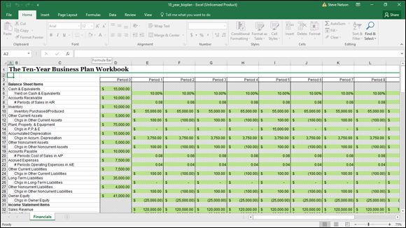
FIGURE 2-1: The inputs area of the business plan workbook.

To use the workbook, you develop and then enter information about the following:

· Assets

· Creditor and owner’s equities at the start of the forecasting horizon

· Expected changes in the assets and equities over the forecasting horizon

· Revenue and expenses for each period on the forecasting horizon

You’re probably wondering how this baby works. Well, the workbook does a lot, but it’s actually pretty straightforward in its operation. When you input data that includes your starting assets, liabilities, owner’s equity balances, and expected changes in these amounts for the forecasting horizon, the workbook constructs a balance sheet. The workbook constructs an income statement when you input data that includes sales and costs of sales, operating expenses, interest income and expenses, and marginal income tax rates. Then, from the balance sheet and income statement, the workbook constructs a cash flow statement.

To enter your own data in the business planning starter workbook, perform the following steps, entering positive balances or increases as positive amounts and negative balances or decreases as negative amounts:

1. Open the business plan workbook, bizplan.xls , from my website by choosing Excel’s File⇒  Open command and then entering http://stephenlnelson.com/wp-content/uploads/10_year_bizplan-1.xlsx in the Filename box.

The starter workbook initially contains the default inputs shown in Figure 2-1 . Note that you can see only about the first 30 rows and the first 12 or so columns of the inputs area. Sorry — I didn’t have room to show everything. If you want to see what you’re missing, grab the workbook from the website.

2. Enter the Cash & Equivalents balance for the start of the forecasting horizon.

The value that you enter for Cash & Equivalents is the dollar total of all the cash held at the beginning of the forecasting period.

You can get the Cash & Equivalents value from QuickBooks if you’re forecasting from the present forward. The cash that you start with, obviously, is the cash that you’re holding today.

3. Enter the forecasted period yield that you expect the cash and equivalents to deliver.

The model estimates the period interest income by multiplying the cash and equivalents balance by the yield on cash and equivalents.

4. Enter the accounts receivable balance for the start of the forecasting horizon.

The value that you enter for accounts receivable (A/R) is the starting accounts receivable balance, which is the balance at the beginning of the forecasting horizon, excluding any allowance for uncollectible amounts.

5. Enter the number of periods of sales in accounts receivable.

The value that you enter for # Periods of Sales in A/R, or number of periods of sales in accounts receivable, is the number of periods or the fraction of a period for which sales are held in accounts receivable. If accounts receivable typically amount to about 30 days of sales, and you use months as your forecasting periods, you hold one period (one month) of sales in accounts receivable. Alternatively, if accounts receivable typically amount to about 30 days of sales, and you use years as your forecasting periods, you hold one twelfth of a period of sales in accounts receivable.

6. Enter the dollar amount of the inventory held at the start of the forecasting horizon.

The Inventory value is the starting inventory balance, which is the total dollar amount of the inventory purchased for resale or manufactured for resale and held at the beginning of the forecasting horizon.

7. Enter the forecasted dollar amount of inventory purchased or produced for each period of the forecasting horizon.

The Inventory Purchased/Produced value is the dollar total of items purchased or produced over the period.

8. Enter the amount of the other current assets held at the start of the forecasting horizon.

The Other Current Assets starting balance is the dollar total of any other current assets with which you begin the forecasting horizon. These other current assets may include prepaid expenses, short-term investments, and deposits made with vendors.

9. Enter the amount of the change in the other current assets for each period in the forecasting horizon.

The value for Chgs in Other Current Assets, or changes in other current assets for the period, is the dollar total of increases or decreases in the accounts included in the starting Other Current Assets balance.

10.Enter the amount of the plant, property, and equipment at the start of the forecasting horizon.

The starting Plant, Property, & Equipment balance is the dollar total of the fixed assets. This amount includes such items as real estate, manufacturing equipment, furniture, and the Learjet.

11.Enter the amount of the change in plant, property, and equipment (P, P, & E) for each period of the forecasting horizon.

The Chgs in P, P, & E value is the dollar total of decreases or increases in the plant, property, and equipment accounts for the period. Increases in these accounts probably stem from purchases of additional fixed assets. Decreases in these accounts probably stem from disposal of assets.

12.Enter the amount of the accumulated depreciation on plant, property, and equipment at the start of the forecasting horizon.

The starting Accumulated Depreciation balance represents the depreciation expenses charged to date on the assets identified in the starting P, P, & E balance.

13.Enter the amount of the change in the accumulated depreciation for each period of the forecasting horizon.

The Chgs in Accum. Depreciation value is the dollar total of increases and decreases in the accumulated depreciation account for the period. Increases in the accumulated depreciation balance probably stem from the current-period depreciation expense. Decreases in the accumulated depreciation balance probably stem from removing the accumulated depreciation attributed to a fixed asset that you disposed of.

14.Enter the amount of the other noncurrent assets at the start of the period.

The starting Other Noncurrent Assets balance is the dollar total of all other noncurrent assets held at the start of the forecasting period. Other noncurrent assets may include copyrights, patents, and goodwill.

15.Enter the amount of the change in the other noncurrent assets for each period of the forecasting horizon.

The Chgs in Other Noncurrent Assets value is the dollar total increase or decrease for the period in the accounts included in the starting Other Noncurrent Assets balance.

16.Enter the amount of the accounts payable balance at the start of the forecasting horizon.

The starting Accounts Payable (A/P) balance is the dollar total of amounts owed vendors for inventory at the start of the forecasting horizon. This starter workbook calculates future Accounts Payable balances based on the cost of sales volumes. To add precision to the forecasts of accounts payable, the model assumes that accounts payable represent debt incurred for the cost of sales.

17.Enter the number of periods of the cost of sales in accounts payable.

The # Periods Cost of Sales in A/P entry is the number of periods or the fraction of a period for which the cost of sales is held in accounts payable. If accounts payable typically amount to about 30 days of cost of sales, and you use months as your forecasting periods, you hold one period (one month) of cost of sales in accounts payable. Alternatively, if accounts payable typically amount to about 30 days of cost of sales, and you use years as your forecasting periods, you hold one twelfth of a period of cost of sales in accounts payable.

18.Enter the amount of the accrued expenses balance at the start of the forecasting horizon.

The starting Accrued Expenses (A/E) balance is the dollar total of amounts owed vendors for operating expenses at the start of the forecast horizon. This starter workbook calculates future Accrued Expenses balances based on the operating expenses levels. To add precision to the forecasts of accrued expenses, the model assumes that accrued expenses represent debt incurred for operating expenses.

19.Enter the number of periods of operating expenses in accrued expenses.

The # Periods Operating Expenses in A/E value is the number of periods or the fraction of a period for which operating expenses are held in accrued expenses. If accrued expenses typically amount to 30 days of operating expenses, and you use months as your forecasting periods, you hold one period of operating expenses in accrued expenses. Alternatively, if accrued expenses typically amount to about 30 days of operating expenses, and you use years as your forecasting periods, you hold one twelfth of a period of operating expenses in accrued expenses.

20.Enter the amount of the other current liabilities at the start of the forecasting period.

The Other Current Liabilities starting balance is the dollar total of all other current liabilities held at the start of the forecasting period. Other current liabilities may include income tax payable, product warranty liability, and the current portion of a long-term liability.

21.Enter the amount of the change in the other current liabilities for each period of the forecasting horizon.

The Chgs in Other Current Liabilities value is the dollar total of increases or decreases for the period in the accounts included in the starting Other Current Liabilities balance.

22.Enter the amount of the long-term liabilities balance at the start of the forecasting horizon.

The starting Long-Term Liabilities balance is the dollar total of debt that will be paid back sometime after the next year.

23.Enter the amount of the change in the long-term liabilities for each period of the forecasting horizon.

The Chgs in Long-Term Liabilities value is the increase or decrease for the period in the outstanding long-term debt. These changes may include decreases stemming from the amortization of principal through debt service payments and increases stemming from additional funds provided by creditors. You need to include the principal component of debt service payments as negative amounts because they decrease the amount of long-term liability.

24.Enter the amount of the other noncurrent liabilities at the start of the forecasting horizon.

The Other Noncurrent Liabilities starting balance is the dollar total of all other noncurrent liabilities held at the start of the forecasting period. These may include deferred income tax, employee pension plan liabilities, and capitalized lease obligations.

25.Enter the amount of the change in the other noncurrent liabilities for each period of the forecasting horizon.

The Chgs in Other Noncurrent Liabilities value is the dollar total of increases or decreases for the period in the accounts included in the starting Other Noncurrent Liabilities balance. These changes may include decreases stemming from the amortization of principal through debt service payments and increases stemming from additional funds provided by creditors.

26.Enter the amount of the owner’s equity balance at the start of the forecasting horizon.

The Owner Equity starting balance is the dollar total of the capital originally contributed by owners and the earnings retained by the business at the start of the forecasting horizon.

27.Enter the amount of the change in the owner’s equity balance for each period of the forecasting horizon stemming from additional capital contributions, dividends, and other special distributions to owners.

The Chgs in Owner Equity value is the dollar total of increases for the period in owner’s equity, other than those stemming from the profits of a business, and all decreases in owner’s equity. Increases in the Owner Equity balance may result from additional offerings of common or preferred stock and Treasury stock transactions; decreases in the Owner Equity balance may result from dividends and other distributions to stockholders.

Changes to the owner’s equity balance resulting from the profit or loss for the period are calculated on the income statement; they aren’t entered.

28.Enter the sales revenue forecasted for each period of the forecasting horizon.

The Sales Revenue values represent the forecasted sales revenues generated by the business over each period of the forecasting horizon.

29.Enter the cost of sales forecasted for each period of the forecasting horizon.

The Cost of Sales values represent the forecasted costs of the inventory sold for the forecasting horizon.

30.Enter those costs that fall into the first, second, and third operating expense classifications or categories for each period of the forecasting horizon.

The operating expenses for Cost Centers 1, 2, and 3 represent the operating expenses for the forecasting horizon. These figures may be three expense classifications related to operating the business, or they may be the total expenses for three groups of expenses.

Typically, you’d use one cost center to track your general and administrative expenses, another cost center to track your sales and marketing expenses, and yet another cost center to track your research and development expenses. If you do this, consider replacing the labels Cost Center 1, Cost Center 2, and Cost Center 3 with more descriptive and meaningful labels, such as General & Admin, Sales & Marketing, and Research & Development.

31.Enter the interest expense of carrying any debt used to fund operations or asset purchases.

The Interest Expense values represent the period interest expenses of carrying any debt related to the business.

32.Enter the income tax rate that, when multiplied against the profit or loss for the period, calculates the income tax expense (or savings).

The Income Tax Rate value is the percentage that, when multiplied by the operating profit (or loss), calculates the income tax expense (or savings). This can be a little tricky because business income taxes are progressive. A sole proprietor’s tax rates go from 0 to roughly 35 percent, for example, depending on the level of income. A regular corporation’s income tax rates go from 15 to 34 percent (with some bounces up and down along the way). This may mean that you need your tax adviser’s help to come up with a good number for this input. On the other hand, you may just decide to calculate only pre-tax profits and losses. To do this, enter this amount as 0.

After you enter the required inputs, the starter workbook makes the calculations necessary to construct pro forma financial statements and to calculate a set of rather standard financial ratios.

Understanding the Workbook Calculations

The business plan workbook has seven parts: the inputs forecast, Balance Sheet, Common Size Balance Sheet, Income Statement, Common Size Income Statement, Cash Flow Statement, and Financial Ratios Table. I want to briefly describe the Excel calculations that occur within each of these parts so that in case you have questions about them or want to make modifications, you can customize the starter workbook to perform better for your specific situation.

If you don’t know Excel and don’t want to learn it, don’t worry. You can just skip this discussion. I provide it for the benefit of those readers who want to understand the inner workings of the workbook and may need or want to customize the workbook’s calculations.

Forecasting inputs

The inputs area of the business planning starter workbook contains one set of formulas. The second row identifies the period for which the results are calculated. The period identifier numbers the periods for which values are entered. The start of the first period is stored in cell D3 as the integer 0. Periods that follow are stored as the previous period plus 1.

The period identifiers in the Balance Sheet, Common Size Balance Sheet, Income Statement, Cash Flow Statement, and Financial Ratios Table schedules use similar formulas.

The cells that hold the period identifiers use a custom number format that precedes each period with the word Period. To remove this, simply reformat the cells by using another number format. You can most easily do this by selecting a cell and then clicking a formatting button on the Excel toolbar, such as the Currency or Percent Style button.

Balance Sheet

The Balance Sheet schedule has 19 rows with calculated data, but the first row contains only text labels that reflect period numbers, shown in Figure 2-2 . (As in the inputs area of the business planning starter workbook, the period identifier numbers the periods for which values are forecasted.) The rest of the Balance Sheet’s values are described in the following paragraphs.

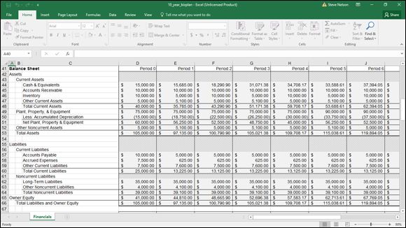
FIGURE 2-2: The Balance Sheet portion of the business planning starter workbook.

Cash & Equivalents

The Cash & Equivalents figures show the projected cash on hand at the end of each of the forecasting periods. The starting balance is the value you enter in the inputs area of the business planning starter workbook. The balance for the first and subsequent periods is pulled from the Cash Flow Statement schedule, where it’s calculated.

Accounts Receivable

The Accounts Receivable (A/R) figures show the net receivables held as of the end of each forecasting period. The starting balance is the value that you enter in the inputs planning area of the business starter worksheet. The balance for the first and subsequent periods is based on the Sales Revenue and the # Periods of Sales in A/R values that you enter in the inputs area of the business planning starter workbook. The formula for the first period is

=E8*E32

The formula for the second period is

=F8*F32

and so on.

Inventory

The Inventory values show the dollar total of the inventory held at the end of each forecasting period. The starting balance is the value that you enter in the inputs area of the business planning starter workbook. The balance for the first and subsequent periods is the previous-period balance plus any inventory purchases or production costs minus any cost of sales. The formula for the first period is

=D46+E10 - E33

The formula for the second period is

=E46+F10 - F33

and so on.

Other Current Assets

The Other Current Assets figures show the dollar total of the other current assets held at the end of each forecasting period. The starting balance for Other Current Assets is the value that you enter in the inputs area of the business planning starter workbook. The balance for the first and subsequent periods is the previous balance plus the change in the balance. The formula for the first period is

=D47+E12

The formula for the second period is

=E47+F12

and so on.

Total Current Assets

The Total Current Assets figures show the dollar total of the current assets at the end of each of the forecasting horizons. The balance at any time is the sum of Cash & Equivalents, Accounts Receivable, Inventory, and Other Current Assets. The formula for the starting Total Current Assets balance is

=SUM(D44:D47)

The formula for the first period is

=SUM(E44:E47)

and so on.

Plant, Property, & Equipment

The Plant, Property, & Equipment figures show the original dollar cost of the plant, property, and equipment at the end of each forecasting horizon. The starting Plant, Property, & Equipment balance is the value that you enter in the inputs area of the business planning starter workbook. The balance for the first and subsequent periods is the previous balance plus any additions to the plant, property, and equipment accounts. The formula for the first period is

=D49+E14

The formula for the second period is

=E49+F14

and so on.

Less: Accumulated Depreciation

The Accumulated Depreciation figures show the cumulative depreciation expenses charged through the current period for the plant, property, and equipment. The starting balance is the value that you enter in the inputs area of the business planning starter workbook. The balance for the first and subsequent periods is the previous balance minus the current period’s changes in accumulated depreciation. The formula for the first period is

=D50 - E16

The formula for the second period is

=E50 - F16

and so on. Because the accumulated depreciation is shown as a negative amount, you subtract the positive number pulled from the forecasting inputs.

Net Plant, Property, & Equipment

The Net Plant, Property, & Equipment figures show the difference between Plant, Property, & Equipment and Accumulated Depreciation at the end of each of the forecasting horizons. The formula for the starting balance is

=D49+D50

The formula for the first period is

=E49+E50

and so on. Because the Accumulated Depreciation balance is shown as a negative amount, you simply add these two amounts in the formula for the Net Plant, Property, & Equipment amount.

Other Noncurrent Assets

The Other Noncurrent Assets figures show the dollar total of any other noncurrent assets held at the end of each forecasting period. The starting balance is the value that you enter in the inputs area of the business planning starter workbook. The balance for the first and subsequent periods is the previous-period balance plus the change in the account in the current period. The formula for the first period is

=D52+E18

The formula for the second period is

=E52+F18

and so on.

Total Assets

The Total Assets figures show the dollar total of all the assets held at the end of the forecasting periods. The balance at any time is the sum of the following: Current Assets; Net Plant, Property, & Equipment; and Other Noncurrent Assets. The formula for the starting balance is

=D48+D51+D52

The formula for the first period is

=E48+E51+E52

and so on.

Accounts Payable

The Accounts Payable figures show the debt that is related to the cost of sales outstanding at the end of each forecasting period. The starting balance is the value that you enter in the inputs area of the business planning starter workbook. The balance for the first and subsequent periods is Cost of Sales for the period times # Periods Cost of Sales In A/P. The formula for the first period is

=E20*E33

The formula for the second period is

=F20*F33

and so on.

Accrued Expenses

The Accrued Expenses figures show the debt that is related to the operating expenses outstanding at the end of each forecasting period. The starting balance is the value that you enter in the inputs area of the business planning starter workbook. The balance for the first and subsequent periods is the operating expenses times # Periods Operating Expenses in A/E. The formula for the first period is

=E22*SUM(E34:E36)

The formula for the second period is

=F22*SUM(F34:F36)

and so on.

Other Current Liabilities

The Other Current Liabilities figures show the dollar total of other debts outstanding at the end of the forecasting periods that will be paid within the current year or business cycle. The starting balance is the value that you enter in the inputs area of the business planning starter workbook. The balance for the first and subsequent periods is the previous balance plus the change in the current period. The formula for the first period is

=D59+E24

The formula for the second period is

=E59+F24

and so on.

Total Current Liabilities

The Total Current Liabilities figures show the dollar total of all the current liabilities at the end of each forecasting period. The balance at any time is the sum of Accounts Payable, Accrued Expenses, and Other Current Liabilities. The formula for the starting balance is

=SUM(D57:D59)

The formula for the first period is

=SUM(E57:E59)

and so on.

Long-Term Liabilities

The Long-Term Liabilities figures show the dollar total of the long-term outstanding debt at the end of each forecasting period. The starting balance is the value that you enter in the inputs area of the business planning starter workbook. The balance for the first and subsequent periods is the previous balance plus any changes in the Long-Term Liabilities balance in the current period. The formula for the first period is

=D62+E26

The formula for the second period is

=E62+F26

and so on.

Other Noncurrent Liabilities

The Other Noncurrent Liabilities figures show the dollar total of any other noncurrent outstanding debt at the end of each forecasting period. The starting balance is the value that you enter in the inputs area of the business planning starter workbook. The balance for the first and subsequent periods is the previous-period balance plus the change in the current period. The formula for the first period is

=D63+E28

The formula for the second period is

=E63+F28

and so on.

Total Noncurrent Liabilities

The Total Noncurrent Liabilities figures show the dollar totals of the long-term debt and the other noncurrent outstanding debt at the end of each forecasting period. The balance at any time is the sum of Long-Term Liabilities and Other Noncurrent Liabilities. The formula for the starting balance is

=D62+D63

The formula for the first period is

=E62+E63

and so on.

Owner Equity

The Owner Equity figures show the dollar totals of the owner’s equity accounts at the end of each forecasting period. The starting balance is the value that you enter in the inputs area of the business planning starter workbook. The balance for the first and subsequent periods is the previous-period balance plus Net Income After Taxes for the period, plus other adjustments, such as additional capital contributions and dividends. The formula for the first period is

=D65+E30+E113

The formula for the second period is

=E65+F30+F113

and so on.

Total Liabilities and Owner Equity

The Total Liabilities and Owner Equity figures show the dollar totals of Current Liabilities, Noncurrent Liabilities, and Owner Equity at the end of each forecasting period. The formula for the starting balance is

=D60+D64+D65

The formula for the first period is

=E60+E64+E65

and so on.

The Total Assets value should equal the Total Liabilities and Owner Equity value. If they differ, your model contains an error.

Common Size Balance Sheet

The Common Size Balance Sheet schedule lists — in the balance sheet format — what percentage of the total assets each individual asset represents and what percentage of the total liabilities and owner’s equity each individual liability and the owner’s equity represents, as shown in Figure 2-3 . When you compare these percentages with those of business peers, you can see the relative financial strength or weakness of your business. Trends in the percentages over time can indicate improvement or deterioration in the overall financial condition of your business.

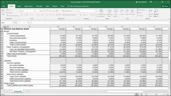
FIGURE 2-3: The Common Size Balance Sheet portion of the business plan workbook.

The Common Size Balance Sheet schedule has 19 rows with calculated data that express line-item amounts as percentages of the total. For the asset side of the Balance Sheet, assets are expressed as a percentage of the total assets. For the creditor and owner’s equity side of the Balance Sheet, equities are expressed as a percentage of the total liabilities and owner’s equity. The formulas for all rows except Total Assets and Total Liabilities and Owner Equity simply convert the Balance Sheet values to percentages. The Cash & Equivalents formula for the starting period is

=D44/D$53

The formula for the first period is

=E44/E$53

and so on. All asset percentages are derived from dividing by Total Assets, which explains why the absolute reference to row $52 is used in all asset formulas. Similarly, the absolute reference to row $66 appears in all formulas in the liabilities and equity formulas.

The formula for the Total Assets percentage at any time is the sum of the Current Assets percentage; the Net Plant, Property & Equipment percentage; and the Other Noncurrent Assets percentage. The result always equals 100 percent.

Similarly, the formula for the Total Liabilities and Owner Equity percentage at any time is the sum of the Current Liabilities, the Noncurrent Liabilities, and Owner Equity percentages. The result is always 100 percent.

Income Statement

The Income Statement schedule has 13 rows of calculated data, as shown in Figure 2-4 . As in other schedules, the period identifier simply numbers the periods for which values are calculated. The first period is stored in cell E96 as the integer 1, and the periods that follow are stored as the previous period plus 1. The other values in the Income Statement are calculated as described in the following paragraphs.

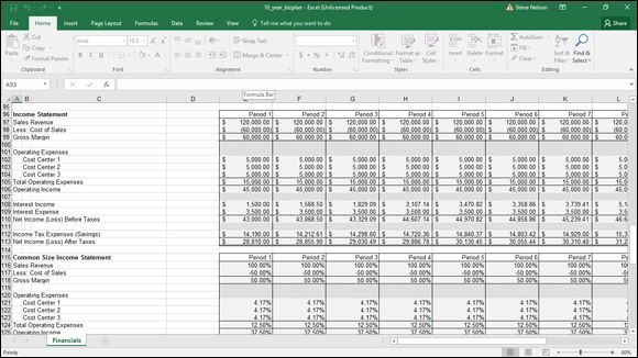
FIGURE 2-4: The Income Statement and the first few rows of the Common Size Income Statement.

Sales Revenue

The Sales Revenue figures are the estimates that you enter in the inputs area of the business planning starter workbook. The amount for the period is the value that you enter in the inputs area of the business planning starter workbook.

Less: Cost of Sales

The Cost of Sales figures are the Cost of Sales estimates that you enter in the inputs area of the business planning starter workbook.

Gross Margin

The Gross Margin figures show the amounts left over from the sales proceeds after subtracting Cost of Sales. Subtracting your other expenses from the Gross Margin amount gives you your profit figure. The Gross Margin formula is Sales Revenue for the period minus Cost of Sales. The formula for the first period is

=E97+E98

The formula for the second period is

=F97+F98

and so on. Notice that because the Cost of Sales figures are pulled into the Income Statement schedule as negative amounts, the Gross Margin formula simply adds the Sales Revenue figure to the negative Cost of Sales figure.

Operating Expenses: Cost Centers 1, 2, and 3

The Operating Expenses figures for Cost Centers 1, 2, and 3 show the amount for each operating expense classification or category that you enter in the inputs area of the business planning starter workbook.

Total Operating Expenses

The Total Operating Expenses figures show the sums of the operating expenses that you enter in the inputs area of the business planning starter workbook for these three operating-expense categories or classifications. The total for each period is the sum of the operating expenses for Cost Centers 1, 2, and 3. The formula for the first period is

=SUM(E102:E104)

The formula for the second period is

=SUM(F102:F104)

and so on.

Operating Income

The Operating Income figures show the sales dollar amounts left after paying the Cost of Sales and the Operating Expenses. The Operating Income figures represent the amounts that go toward paying your financing expenses and income tax, as well as the amount that constitutes your profits. The amount for each period is the Gross Margin figure for the period minus the Total Operating Expenses figure. The formula for the first period is

=E99 - E105

The formula for the second period is

=F99 - F105

and so on.

Interest Income

The Interest Income figures show the earnings from investing the cash of the business. The amount for each period is the beginning Cash & Equivalents balance from the inputs area of the business planning starter workbook multiplied by the period yield on Cash & Equivalents. The formula for the first period is

=D44*E6

The formula for the second period is

=E44*F6

and so on.

Interest Expense

The Interest Expense figures show the costs of using borrowed funds for operations and asset purchases. The amount for each period is the value that you enter in the inputs area of the business planning starter workbook.

Net Income (Loss) Before Taxes

The Net Income (Loss) Before Taxes figures show the amount of operating income left after receiving any interest income and paying any interest expense. The amount for each period is the Operating Income figure for the period plus the Interest Income figure for the period, minus the Interest Expense figure for the period. The formula for the first period is

=E106+E108 - E109

The formula for the second period is

=F106+F108 - F109

and so on.

Income Tax Expenses (Savings)

The Income Tax Expenses (Savings) figures show the income tax expenses (or savings) that use the calculated Net Income (Loss) Before Taxes figures and the Marginal Income Tax Rate figures that you forecasted in the inputs area of the business planning starter workbook. Notice that the model calculates a current period savings in income taxes when there’s a net loss before taxes. This may be the case when a current-period loss is carried back to a previous period or when the current-period loss is consolidated with the current-period income of related businesses. Basically, then, the model assumes that a net loss before income taxes results in a current-period tax refund — that is, an overall tax savings — because you can deduct a loss in one business from the profits of another business. If a current-period loss doesn’t result in a current-period income tax savings, however, you modify the formula as described in “Customizing the Starter Workbook ” later in this chapter.

The amount for each period is the Net Income (Loss) Before Taxes multiplied by the Marginal Income Tax Rate figure. The formula for the first period is

=E38*E110

The formula for the second period is

=F38*F110

and so on.

Net Income (Loss) After Taxes

The Net Income (Loss) After Taxes figures calculate the after-tax profits of operating the business. The amount for each period is the Net Income (Loss) Before Taxes figure minus the Income Tax Expenses (Savings) figure. The formula for the first period is

=E110 - E112

The formula for the second period is

=F110 - F112

and so on.

Common Size Income Statement

The Common Size Income Statement schedule lists, in income statement format, what percentage of the total sales revenue each income statement line item represents (refer to the bottom of Figure 2-4 ). When you compare these percentages with those of business peers, you can see the relative financial performance of your business. Trends in the percentages over the forecasting horizon can indicate improvement or deterioration in the financial performance of your business.

The Common Size Income Statement schedule has 13 rows of calculated data that express the component line-item amount for each period as a percentage of the sales revenue figure for the period. The formulas for all rows except Sales Revenue simply convert the Income Statement values to percentages.

The Sales Revenue figures add the Cost of Sales, Total Operating Expenses, Interest Income, Interest Expense, Income Tax Expenses (Savings), and Net Income (Loss) After Taxes percentages. The results always equal 100 percent.

The Sales Revenue percentage calculations add the expense and profit percentages. Those expenses shown as negative amounts, therefore, are subtracted.

Cash Flow Statement

The Cash Flow Statement schedule has 16 rows of calculated data, shown in Figure 2-5 . As in other schedules, a period identifier numbers the periods for which values are calculated. The first period is stored in cell E136 as integer 1. Periods that follow are stored as the previous period plus 1. Other Cash Flow Statement values are calculated as described in the following paragraphs.

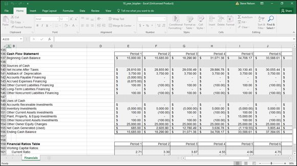
FIGURE 2-5: The Cash Flow Statement and the first few rows of the Financial Ratios Table.

Beginning Cash Balance

The Beginning Cash Balance figures show the forecasted cash and equivalents balance at the start of each forecasting period. The starting balance is the value that you enter in the inputs area of the business planning starter workbook. For subsequent periods, the Beginning Cash Balance is the previous period’s Ending Cash Balance.

Net Income After Taxes

The Net Income After Taxes figures show the amounts calculated in the Income Statement schedule as the business profits for each forecasting period.

Addback of Depreciation

The Addback of Depreciation figures show the change in the accumulated depreciation balance for each forecasting period. Normally, this change stems from the period depreciation expense; it must be added back into the Net Income After Taxes figure because the depreciation expense uses no cash. The depreciation added back for each period is the value that you enter in the inputs area of the business planning starter workbook as the change in accumulated depreciation.

Accounts Payable Financing

The Accounts Payable Financing figures show the change in the Accounts Payable balance for the period. Increases in this balance result when the cost of sales expense paid during the period is lower than the expense incurred. Decreases in this balance result when the cost of sales expense paid is higher than the expense incurred. By recognizing the changes in this account balance, the model adjusts for differences between the Income Statement’s accrual-based accounting of cost of sales expenses and the actual cash disbursements for cost of sales expenses.

The Accounts Payable Financing figure for each period is the difference between the Accounts Payable balance at the end of the previous period and the balance at the end of the current period. The formula for the first period is

=E57 - D57

The formula for the second period is

=F57 - E57

and so on.

Accrued Expenses Financing

The Accrued Expenses Financing figures show the change in the accrued expenses balance for the period. Increases in this balance result when the operating expense paid during the period is lower than the expense incurred. Decreases in this balance result when the operating expense paid during the period is higher than the expense incurred. By recognizing the changes in this account balance, the model adjusts for differences between the Income Statement’s accrual-based accounting expenses and the actual cash disbursements for operating expenses.

The Accrued Expenses Financing figure for each period is the difference between the Accrued Expenses balance at the end of the previous period and the balance at the end of the current period. The formula for the first period is

=E58 - D58

The formula for the second period is

=F58 - E58

and so on.

Other Current Liabilities Financing

The Other Current Liabilities Financing figures show the change in the Other Current Liabilities balance for the period. This amount increases when, either directly or indirectly, cash is generated by borrowing. This amount decreases when, either directly or indirectly, cash is used to pay off short-term borrowing.

The Other Current Liabilities Financing figure for each period is the difference between the Other Current Liabilities balance at the end of the previous period and the balance at the end of the current period. The formula for the first period is

=E59 - D59

The formula for the second period is

=F59 - E59

and so on.

Long-Term Liabilities Financing

The Long-Term Liabilities Financing figures show the changes in the long-term liabilities amount for the period. This balance increases when, either directly or indirectly, cash is generated by long-term borrowing. This amount decreases when, either directly or indirectly, cash is used to pay off long-term borrowing.

The Long-Term Liabilities Financing figure for each period is the difference between the Long-Term Liabilities balance at the end of the previous period and the balance at the end of the current period. The formula for the first period is

=E62 - D62

The formula for the second period is

=F62 - E62

and so on.

Other Noncurrent Liabilities Financing

The Other Noncurrent Liabilities Financing figures show the changes in the Other Noncurrent Liabilities balance for the period. This amount increases when, either directly or indirectly, cash is generated by other long-term borrowing. This amount decreases when, either directly or indirectly, cash is used to pay off other long-term borrowing.

The Other Noncurrent Liabilities Financing figure for each period is the difference between the Other Noncurrent Liabilities balance at the end of the previous period and the balance at the end of the current period. The formula for the first period is

=E63 - D63

The formula for the second period is

=F63 - E63

and so on.

Accounts Receivable Investments

The Accounts Receivable Investments figures show the change in the Accounts Receivable balance for each forecasting period. This amount increases when the sales revenue collected during the period is less than the revenue recorded. This amount decreases when the sales revenue collected during the period is more than recorded. By recognizing the changes in the account balance, the model adjusts for differences between the income statement’s accrual-based accounting of sales revenues and the actual cash collections for sales.

The Accounts Receivable Investments figure for each period is the difference between the Accounts Receivable balance at the end of the previous period and the balance at the end of the current period. The formula for the first period is

=E45 - D45

The formula for the second period is

=F45 - E45

and so on.

Inventory Investments

The Inventory Investments figures show the change in the inventory balance for each forecasting period. This amount increases when the inventory sold is less than the inventory acquired. This amount decreases when the inventory sold is more than the inventory acquired. By recognizing the changes in this account balance, the model recognizes the cash effects of changing inventory balances.

The Inventory Investments figure for each period is the difference between the Inventory balance at the end of the previous period and the balance at the end of the current period. The formula for the first period is

=E46 - D46

The formula for the second period is

=F46 - E46

and so on.

Other Current Assets Investments

The Other Current Assets Investments figures show the changes in the Other Current Assets balance for the period. This amount increases when, either directly or indirectly, cash is used to acquire current assets. This amount decreases when, either directly or indirectly, cash is generated by converting current assets to cash.

The Other Current Assets Investments figure for each period is the difference between the Other Current Assets balance at the end of the previous period and the balance at the end of the current period. The formula for the first period is

=E47 - D47

The formula for the second period is

=F47 - E47

and so on.

Plant, Property, & Equip Investments

The Plant, Property, & Equip Investments figures show the change in the Plant, Property, & Equipment balance for the period. This amount increases when, either directly or indirectly, cash is used to acquire plants, property, and equipment. This amount decreases when, either directly or indirectly, cash is generated by converting plants, property, and equipment to cash.

The Plant, Property, & Equip Investments figure for each period is the difference between the Plant, Property, & Equipment balance at the end of the previous period and the balance at the end of the current period. The formula for the first period is

=E49 - D49

The formula for the second period is

=F49 - E49

and so on.

Other Noncurrent Assets Investments

The Other Noncurrent Assets Investments figures show the changes in the Other Noncurrent Assets balance for the period. This amount increases when, either directly or indirectly, cash is used to acquire other noncurrent assets. This amount decreases when, either directly or indirectly, cash is generated by converting other noncurrent assets to cash.

The Other Noncurrent Assets Investments figure for each period is the difference between the Other Noncurrent Assets balance at the end of the previous period and the balance at the end of the current period. The formula for the first period is

=E52 - D52

The formula for the second period is

=F52 - E52

and so on.

Other Owner Equity Changes

The Other Owner Equity Changes figures show the cash flows stemming from any additional capital contributions made by the owners to the business or from dividends and other distributions made by the business to the owners. The Other Owner Equity Changes figure for each period is the value that you enter in the inputs area of the business planning starter workbook. The Other Owner Equity Changes figures are pulled into the Uses of Cash section as negative values because a positive change in owner’s equity, such as an additional capital contribution (from a stock offering, for example), doesn’t use cash but provides cash.

Net Cash Generated (Used)

The Net Cash Generated (Used) figures show the total cash flow for each period of the forecasting horizon, based on the listed sources and uses of cash. The amount for each period is the sources of cash for the period less the uses of cash for the period. The formula for the first period is

=SUM(E140:E146) - SUM(E149:E154)

The formula for the second period is

=SUM(F140:F146) - SUM(F149:F154)

and so on.

Ending Cash Balance

The Ending Cash Balance figures show the forecasted cash and equivalents balance at the end of each period. The balance is the Beginning Cash Balance figure for the period plus the Net Cash Generated (Used) figure for the period. The formula for the first period is

=E137+E155

The formula for the second period is

=F137+F155

and so on.

Financial Ratios Table

The Financial Ratios Table has 11 rows of calculated data, as shown in Figure 2-6 . As in other schedules, the period identifier numbers the periods for which values are calculated. The first period is stored in cell E159 as the integer 1, and periods that follow are stored as the previous period plus 1. The other values in the Financial Ratios Table are calculated as described in the following paragraphs.

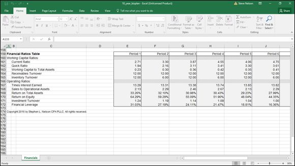
FIGURE 2-6: The Financial Ratios Table.

Current Ratio

The Current Ratio figures show the ratio of current assets to current liabilities. The current ratio provides one measure of a business’s capability to meet its short-term obligations. The Current Ratio figure for each period is the Total Current Assets figure from the Balance Sheet schedule divided by the Total Current Liabilities figure. The formula for the first period is

=E48/E60

The formula for the second period is

=F48/F60

and so on.

Quick Ratio

The Quick Ratio figures show the ratio of the sum of the cash and equivalents plus the accounts receivable to the current liabilities. The quick ratio provides a more stringent measure of a business’s capability to meet its short-term financial obligations than other ratios. The Quick Ratio figure for each period is the sum of the Cash & Equivalents figure and the Accounts Receivable figure divided by the Total Current Liabilities figure. The formula for the first period is

=(E44+E45)/E60

The formula for the second period is

=(F44+F45)/F60

and so on.

Working Capital to Total Assets

The Working Capital to Total Assets figures show the ratio of working capital (the current assets minus the current liabilities) to the total assets. The Working Capital to Total Assets ratio is another measure of a business’s capability to meet its financial obligations and gives an indication as to the distribution of a business’s assets into liquid and nonliquid resources. The Working Capital to Total Assets ratio for each period is calculated by dividing the difference between the Current Assets and Current Liabilities figures by the Total Assets figure. The formula for the first period is

=(E48 - E60)/E53

The formula for the second period is

=(F48 - F60)/F53

and so on.

Receivables Turnover

The Receivables Turnover figures show the ratio of sales to the accounts receivable balance. The Receivables Turnover ratio indicates the efficiency of sales collections. One problem with the measure as it’s usually applied is that both credit and cash sales may be included in the ratio denominator. Two potential shortcomings exist with this approach:

· The presence of the cash sales may make the receivables collections appear more efficient than is the case.

· Mere changes in the mix of credit and cash sales may affect the ratio even though the efficiency of the receivables collections process hasn’t changed.

The Receivables Turnover figure for each period is calculated by dividing the Sales Revenue figure for the period by the Accounts Receivable balance outstanding at the end of the period. The formula for the first period is

=E97/E45

The formula for the second period is

=F97/F45

and so on.

Inventory Turnover

The Inventory Turnover row shows the ratio of the cost of sales to the inventory balance. The Inventory Turnover ratio calculates how long inventory is held. It can indicate depleted or excessive inventory balances. The Inventory Turnover ratio for each period is calculated by dividing the Cost of Sales figure for the period by the inventory held at the end of the period. The formula for the first period is

= - E98/E46

The formula for the second period is

= - F98/F46

and so on.

Times Interest Earned

The Times Interest Earned row shows the ratio of the sum of the net income after taxes plus the interest income to the interest expense. The ratio indicates the relative ease with which the business is paying its financing costs. The Times Interest Earned ratio for each period is calculated by dividing the sum of the Operating Income and Interest Income figures from the Income Statement schedule by the Interest Expense figure. The formula for the first period is

=(E106+E108)/E109

The formula for the second period is

=(F106+F108)/F109

and so on.

Sales to Operational Assets

The Sales to Operational Assets row shows the ratio of sales revenue to net plant, property, and equipment. The ratio indicates the efficiency with which a business uses its operational assets to generate sales revenue. The Sales to Operational Assets ratio for each period is the Sales Revenue figure that you enter in the inputs area of the business planning starter workbook divided by the Net Plant, Property, & Equipment figure from the Balance Sheet schedule. The formula for the first period is

=E97/E51

The formula for the second period is

=F97/F51

and so on.

Return on Total Assets

The Return on Total Assets row shows the ratio of the sum of the net income after taxes plus the interest expense to the total assets for each period. The ratio indicates the overall operating profitability of the business, expressed as a rate of return on the business assets. The formula for the first period is

=(E113+E109)/E53

The formula for the second period is

=(F113+F109)/F53

and so on.

Return on Equity

The Return on Equity row shows the ratio of the net income after taxes to the owner’s equity for each period. The ratio indicates the profitability of the business as an investment of the owners. The Return on Equity ratio for each period is the Net Income (Loss) After Taxes figure from the Income Statement schedule divided by the Owner Equity figure from the Balance Sheet schedule. The formula for the first period is

=E113/E65

The formula for the second period is

=F113/F65

and so on.

Investment Turnover

The Investment Turnover row shows the ratio of the sales revenue to the total assets. The ratio, such as the Sales to Operational Assets ratio, indicates the efficiency with which a business uses its assets (in this case, its total assets) to generate sales. The Investment Turnover ratio for each period is the Sales Revenue figure that you enter in the inputs area of the business planning starter workbook divided by the Total Assets figure from the Balance Sheet schedule. The formula for the first period is

=E97/E53

The formula for the second period is

=F97/F53

and so on.

Financial Leverage

The Financial Leverage row shows the difference between the return on owner’s equity and the return on total assets. The ratio indicates the increase or decrease in an equity return as a result of borrowing. A positive value indicates an improvement in the return on owner’s equity by using financial leverage; a negative value indicates deterioration in the return on owner’s equity. The Financial Leverage figure for each period is the Return on Total Assets figure minus the Return on Equity figure. The formula for the first period is

=E170 - E169

The formula for the second period is

=F170 - F169

and so on.

Customizing the Starter Workbook

You can use the business plan workbook for many business projections, but you may want to change the starter workbook so that it more closely matches your requirements. You can add text that describes your business and the forecasting horizon, for example. You can also increase or decrease the number of periods, perhaps increasing the number of periods to 12 if your periods are months and you want to forecast an entire year.

Before you change anything in the starter workbook other than the forecasting inputs, unprotect the document. To do this, choose the Review tab and click the Unprotect Sheet button.

Unless you turn off cell protection, input cells in the inputs area of the business planning starter workbook are the only cells into which you can enter data.

Changing the number of periods

You can easily increase or decrease the number of forecasting periods.

To increase the number of periods, remove the borders from the last column and then copy the current last column to the right as needed.

To decrease the number of periods, simply delete any unnecessary columns from the right side of the schedule. (To delete a column, highlight the entire column by clicking at the top of that column, right-click to bring up Excel’s shortcut menu, and then choose Delete.) After you finish these steps, you can replace the borders on the right and reinstate cell protection as needed.

Performing ratio analysis on existing financial statements

If you want to perform financial ratio analysis on a set of existing financial statements, copy the contents of column E from the row in the inputs area of the business plan workbook that contains the sales revenue forecast (row 32) through the last row of the ratios table into column D. Then remove the columns for periods 1 through 10 (columns E through N) by following the steps described in “Changing the number of periods ” earlier in this chapter. Optionally, you can delete the Cash Flow Statement and add appropriate column headings as needed.

To use the modified starter workbook, enter the necessary Balance Sheet and Income Statement data in each of the unshaded cells in column D of the inputs area of the business planning starter workbook. (Typically, the As Of date of the Balance Sheet and the ending date of the Income Statement period are the same.)

Calculating taxes for a current net loss before taxes

To calculate the income tax expense as 0 when you have a current period net loss before income taxes, you edit the formula in the cell that calculates the income tax expense (or savings) for the first period (cell E112) so that it takes the maximum of the calculated expense amount or 0 by using the MAX function:

=MAX(E38*E110,0)

After you’ve done this, you can copy the formula into the rest of the cells in the forecasting horizon that calculate the income tax expense (or savings). To do this, select the cell with the formula you want to copy, click the Home button, and then click the Copy button. Next, select the range of cells into which you want to copy the formula, and click the Paste button.

Combining this workbook with other workbooks

A quick and perhaps obvious point: You may want to construct other workbooks to supply numbers to the business plan workbook discussed in this chapter. You can construct an asset depreciation schedule, for example, that uses the straight-line depreciation convention for a $25,000 asset representing your entire plant, property, and equipment investment and then use this data in the business plan workbook.

If you start doing more Excel work, and you’re not all that comfortable with Excel, consider picking up a recent edition of Excel For Dummies, by Greg Harvey (John Wiley & Sons, Inc.). It’s a great tutorial on the basics. Also, if you want more information about constructing supporting financial workbooks (such as an asset depreciation schedule), you may want to visit my website, www.stephenlnelson.com . I provide a freebie version of another book I’ve written, the MBA’s Guide to Microsoft Excel (Redmond Technology Press), that describes how to do tasks like these (see http://stephenlnelson.com/articles/category/excel/ ).

If you want to use workbooks together in this manner, you should probably combine the workbooks into a single workbook. The easiest way to copy one of the workbooks is to copy the workbook’s worksheet to a blank worksheet in the other workbook. (Each of the starter workbooks uses only a single worksheet to make this process both easy and possible.)