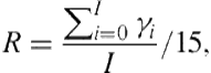
Plan, Activity, and Intent Recognition: Theory and Practice, FIRST EDITION (2014)
Part V. Applications
Chapter 13. Using Opponent Modeling to Adapt Team Play in American Football
Kennard R. Laviersa and Gita Sukthankarb, aAir Force Institute of Technology, Wright Patterson AFB, OH, USA, bUniversity of Central Florida, Orlando, FL, USA
Abstract
An issue with learning effective policies in multiagent adversarial games is that the size of the search space can be prohibitively large when the actions of both teammates and opponents are considered simultaneously. Opponent modeling, predicting an opponent’s actions in advance of execution, is one approach for selecting actions in adversarial settings, but it is often performed in an ad hoc way. This chapter introduces several methods for using opponent modeling, in the form of predictions about the players’ physical movements, to learn team policies. To explore the problem of decision making in multiagent adversarial scenarios, we use our approach for both offline play generation and real-time team response in the Rush 2008 American Football Simulator. Simultaneously predicting movement trajectories, future reward, and play strategies of multiple players in real time is a daunting task, but we illustrate how it is possible to divide and conquer this problem with an assortment of data-driven models.
Keywords
Opponent modeling
American football
Play recognition
Adaptive players
Upper Confidence bounds applied to Trees (UCT)
Acknowledgment
This research was partially supported by National Science Foundation awardIIS-0845159. The views expressed in this document are those of the authors and do not reflect the official policy or position of the U.S. Air Force, Department of Defense, or the government.
13.1 Introduction
In military and athletic environments, agents must depend on coordination to perform joint actions in order to accomplish team objectives. For example, a soldier may signal another soldier to “cover” her while she attempts to relocate to another strategic location. In football, the quarterback depends on other team members to protect him while he waits for a receiver to get into position and to become “open.” Because of these coordination dependencies, multiagent learning algorithms employed in these scenarios must consider each agent’s actions with respect to its teammates’, since even good action selections can fail solely due to teammates’ choices. Team adversarial scenarios are even more complicated because opponents are actively thwarting actions. In the contest of American football, the leading causes for failures are as follows:
• An action is a poor selection for the tactical situation. Example: a player runs too close to a fast opponent and gets tackled.
• Good action choices are not guaranteed to succeed. Example: a player fumbles a well-thrown pass.
• Poor coordination between team members. Example: a ball handoff fails because the receiving player does not run to the correct location.
• Opponents successfully counter the planned action. Example: the defense overcomes the offensive line’s protection scheme, leaving the quarterback unprotected.
Although reward metrics are useful for gauging the performance of a plan or policy, it is impossible to diagnosis the root cause of policy failure based on the reward function alone. Moreover, often the reward metric is sparse, providing little information about intermediate stages in the plan. Even minor miscalculations in action selections among coordinating agents can be very unforgiving, yielding either no reward or a negative reward. Finally, physical agents often operate in continuous action spaces since many of the agent actions are movement-based; sampling or discretizing a large two-dimensional area can still result in a significant increase in the number of action possibilities. In summary, team adversarial problems often pose the following difficulties:
(1) Large and partially continuous search space
(2) Lack of intermediate reward information
(3) Difficulty in identifying action combinations that yield effective team coordination
(4) Constant threat of actions being thwarted by adversaries
This chapter describes a set of methods to improve search processes for planning and learning in adversarial team scenarios. American football was selected as the experimental domain for empirical testing of our work for several reasons. First, American football has a “playbook” governing the formations and conditional plans executed by the players, eliminating the necessity of an unsupervised discovery phase in which plans and templates are identified from raw data. Recognizing the play in advance definitely confers advantages on the opposing team but is not a guarantee of victory. The existence of a playbook distinguishes American football from less structured cooperative games (e.g., first-person shooters).
Additionally, football routinely punishes poor coordination, often yielding significant negative rewards for minor errors among players. It is difficult, if not impossible, to evaluate how well a play is doing until either the ball is received by a receiver or being carried up the field by a running back. We selected the Rush 2008 Football Simulator [26] for our research since it can simulate complex plays yet is sufficiently lightweight to facilitate running machine-learning experiments. It comes with an existing play library, and we developed a sketch-based interface for authoring new plays and a test environment for evaluating machine learning algorithms (shown in Figure 13.1). Our Rush Analyzer and Test Environment (RATE) is designed to facilitate reproducible research on planning and learning in a Rush 2008 football game. RATE consists of more than 40,000 lines of code and has support for separate debugging of AI subsystems, parallel search, and point-and-click configuration.
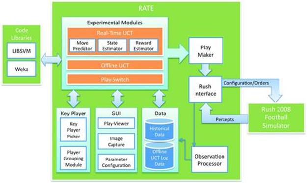
FIGURE 13.1 Rush Analyzer and Test Environment designed to facilitate reproducible research on planning and learning in a Rush 2008 football game.
This chapter focuses on four key research areas:
• The use of opponent modeling/play recognition to guide action selection (Section 13.4)
• Automatically identifying coordination patterns from historical play data (Section 13.5)
• The use of play adaptation (Section 13.5.2) and Monte Carlo search to generate new plays (Section 13.6)
• Incorporating the preceding items with a set of data-driven models for move prediction and reward estimation to produce a football agent that learns in real time how to control the actions of three offensive players for a critical early stage of a play (Section 13.7).
Our system is the first autonomous football game player capable of learning team plan repairs in real time to counter predicted opponent actions.
Although effective opponent modeling is often identified as an important prerequisite for building agents in adversarial domains [42], research efforts have focused mainly on the problem of fast and accurate plan recognition [3,17] while neglecting the issues that occur post-plan recognition. Using opponent modeling to guide the play of an autonomous agent is an intuitively appealing idea for game designers, but one that poses many practical difficulties. The first issue is that many games, particularly ones that involve physical movement of the bots, are relatively unconstrained; often, there is no need for human players to consistently follow a mental playbook. This hampers plan-recognition systems that rely on pregenerated models, libraries, and templates. In contrast, the actions of a human player interacting with the Rush football system are limited since the human is only allowed to control the quarterback; the rest of the team is played autonomously according to a preexisting play library. Additionally, it is easy to segment American football plays since there are breaks in action every time a tackle occurs or the ball is fumbled, compared to soccer in which the action flows more naturally. These qualities make American football well suited for a study of the competitive benefits of play recognition; planning is crucial and accurate plan recognition is possible.
13.2 Related Work
The term “opponent modeling” has been used in a wide variety of contexts, ranging from the prediction of immediate actions to forecasting long-term strategies and intentions. Interestingly, one of the first mentions of opponent modeling in the artificial intelligence (AI) literature pertains to predicting movements in football [25]. In our work, we treat opponent modeling as a specialized version of online team behavior recognition in which our system solves a multiclass classification problem to identify the currently executing play.
Previous work on recognizing and analyzing team behaviors has been largely evaluated within athletic domains, not just in American football [15] but also basketball [5,16] and Robocup soccer [31,32,20]. In Robocup, a majority of the research on team behavior recognition has been done for the coach competition. The aim of the competitors is to create autonomous agents that can observe game play from the sidelines and provide strategy advice to a team in a specialized coaching language. Techniques have been developed to extract specific information (e.g., home areas [33], opponent positions during set plays [32], and adversarial models [31]) from logs of Robocup simulation league games. This information can be used by the coaching agent to improve the team’s scoring performance. For instance, information about opponent agent home areas can be used as triggers for coaching advice and for doing “formation-based marking” in which different team members are assigned to track members of the opposing team. While the focus of the coaching agent is to improve performance of teams in future games, our system takes action immediately after recognizing the play to search for possible action improvements.
One of the other book chapters describes a new direction in Robocup research—the creation of ad hoc teams [13]. In role-based ad hoc teams, the new agent studies the behavior of its future teammates before deciding on a policy based on marginal utility calculations. Our play-adaptation system does a holistic analysis of team performance based on past yardage gained rather than disentangling the relative contributions of individual agents toward the overall success of the play.
A related line of Robocup research is the development of commentator systems that provide natural language summaries describing action on the field. For instance, the Multiagent Interactions Knowledgeably Explained (MIKE) system used a set of specialized game analysis modules for deciphering the meaning of spatiotemporal events, including a bigram module for modeling ball plays as a first-order Markov chain and a Voronoi module for analyzing defense areas [39]. MIKE was one of three similar commentator systems (along with Rocco and Byrne) that received scientific awards in Robocup 1998 [44].
While commentator systems focus on producing real-time dialog describing game play, automated team analysis assistants are used to do post hoc analysis on game logs [40]. One of the earliest systems, ISAAC, learned decision trees to characterize the outcome of plays and also possessed an interactive mode allowing the team designer to explore hypothetical modifications to the agent’s parameters [28]. This style of analysis has been successfully applied to real-world NBA basketball data in the Advanced Scout system [5], which was later commercialized by VirtualGold. These data mining tools have a knowledge discovery phase where patterns in the statistics of individual players (e.g., shooting performance) are identified. Interpreted results are presented to the coaching staff in the form of text descriptions and video snippets. Our system directly channels information about past performance of plays into dynamically adapting the actions of the offensive team and also learning offline plays. The knowledge discovery phase in our work is assumed to be supervised by a knowledgeable observer who tags the plays with labels, rather than being performed in an unsupervised fashion.
One of the earliest camera-based sports analysis systems was developed for the football domain [15]. In addition to performing low-level field rectification and trajectory extraction, it recognizes football plays using belief networks to identify actions from accumulated visual evidence. Real-world football formations have been successfully extracted from snapshots of football games by Hess et al., who demonstrated the use of a pictorial structure model [14]. Kang et al. demonstrated the use of Support Vector Machines (SVM) to detect scoring events and track the ball in a soccer match [18,30]. Visual information from a post-mounted camera outside the soccer field was used to train the SVMs. For our opponent modeling, we use multiclass SVMs to classify the defensive team plays based on observation logs using a training method similar to the one of Sukthankar and Sycara [37].
Note that the use of opponent modeling to guide action selection carries the inherent risk of being “bluffed” into poor actions by a clever opponent tricking the system into learning a false behavior model. In football, running plays are more effective if the opponent can be fooled into believing that the play is actually a passing play. Smart human players often engage in recursive thinking and consider what the opponent thinks and knows as well as the observed actions [6]. The interactive partially observable Markov decision process (I-POMDP) framework explicitly models this mode of adversarial thinking (see Doshi et al.’s chapter in this book [11] for a more detailed description). In this work, we do not consider the mental factors that affect the choice of play, only post-play adaptations.
13.3 Rush Football
The goal is to produce a challenging and fun computer player for the Rush 2008 football game, developed by Knexus Research [26], capable of responding to a human player in novel and unexpected ways. In Rush 2008, play instructions are similar to a conditional plan and include choice points where the players can make individual decisions as well as predefined behaviors that the players execute to the best of their physical capability. Planning is accomplished before a play is enacted, and the best plays are cached in a playbook. Certain defensive plays can effectively counter specific offenses. Once the play commences, it is possible to recognize the defensive play and to anticipate the imminent failure of the offensive play.
American football is a contest of two teams played on a rectangular field. Unlike standard American football, which has 11 players on a team, Rush teams only have 8 players simultaneously on the field out of a total roster of 18 players, and the field is ![]() yards. The game’s objective is to outscore the opponent, where the offense (i.e., the team with possession of the ball) attempts to advance the ball from the line of scrimmage into the opponent’s end zone. In a full game, the offensive team has four attempts to get afirst down by moving the ball 10 yards down the field. If the ball is intercepted or fumbled and claimed by the defense, ball possession transfers to the defensive team. Stochasticity exists in many aspects of the game including throwing, catching, fumbling, blocking, running, and tackling. Our work mainly focuses on improving offensive team performance in executing passing plays.
yards. The game’s objective is to outscore the opponent, where the offense (i.e., the team with possession of the ball) attempts to advance the ball from the line of scrimmage into the opponent’s end zone. In a full game, the offensive team has four attempts to get afirst down by moving the ball 10 yards down the field. If the ball is intercepted or fumbled and claimed by the defense, ball possession transfers to the defensive team. Stochasticity exists in many aspects of the game including throwing, catching, fumbling, blocking, running, and tackling. Our work mainly focuses on improving offensive team performance in executing passing plays.
In American football, the offensive lineup consists of the following positions:
Quarterback (QB): given the ball at the start of each play and initiates either a run or a pass.
Running back (RB): begins in the backfield, behind the line of scrimmage where the ball is placed, with the QB and FB. The running back is eligible to receive a handoff, backward pitch, or forward pass from the QB.
Fullback (FB): serves largely the same function as the RB.
Wide receiver (WR): the primary receiver for pass plays. This player initially starts near the line of scrimmage but on the far right or far left of the field.
Tight end (TE): begins on the line of scrimmage immediately to the outside of the OL and can receive passes.
Offensive lineman (OL): begins on the line of scrimmage and is primarily responsible for preventing the defense from reaching the ball carrier.
A defensive lineup has the following positions:
Defensive lineman (DL): line up across the line of scrimmage from the OL and focuses on tackling the ball handler as quickly as possible.
Linebackers (LB): line up behind the lineman and can blitz the opposing QB by quickly running toward him en masse. Often their role is to guard a particular zone of the playing field or an eligible receiver, depending on whether they are executing a zone or a man defense.
Cornerbacks (CB): typically line up across the line of scrimmage from the wide receivers. Their primary responsibility is to cover the WR.
Safety (S): lines up far behind the line of scrimmage. They typically assist with pass coverage but, like all defensive players, can also blitz and can contribute on tackling any ball handler.
A Rush play is composed of (1) a starting formation and (2) instructions for each player in that formation. A formation is a set of ![]() offsets from the center of the line of scrimmage. By default, instructions for each player consist of (a) an offset/destination point on the field to run to and (b) a behavior to execute when they get there. Rush includes three offensive formations (power, pro, and split) and four defensive ones (23, 31, 2222, 2231). Each formation has eight different plays (numbered 1-8) that can be executed from that formation. Offensive plays typically include a handoff to the running back/fullback or a pass executed by the QB to one of the receivers, along with instructions for a running pattern to be followed by all the receivers. Figure 13.2 shows an example play from thePro formation:
offsets from the center of the line of scrimmage. By default, instructions for each player consist of (a) an offset/destination point on the field to run to and (b) a behavior to execute when they get there. Rush includes three offensive formations (power, pro, and split) and four defensive ones (23, 31, 2222, 2231). Each formation has eight different plays (numbered 1-8) that can be executed from that formation. Offensive plays typically include a handoff to the running back/fullback or a pass executed by the QB to one of the receivers, along with instructions for a running pattern to be followed by all the receivers. Figure 13.2 shows an example play from thePro formation:
1. The QB passes to an open receiver
2. The RB and left WR run hook routes
3. The left and right guards pass block for the ball holder
4. The other players wait
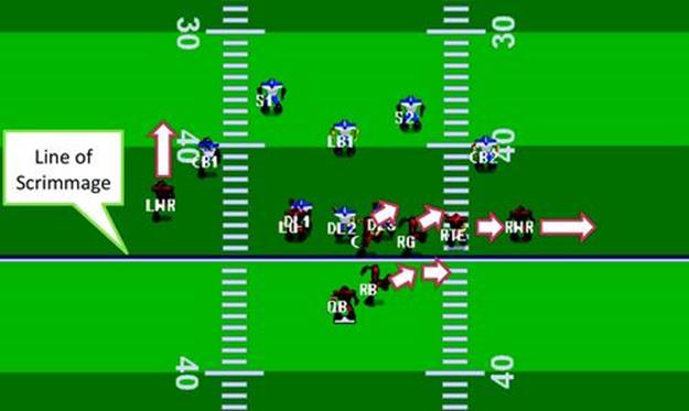
FIGURE 13.2 The Pro formation running play variant 4 against defensive formation 31 running variant 2.
The default Rush playbook contains 24 offensive and 32 defensive plays. Playbooks for real-world football teams are limited by the ability of the players to reliably learn and execute the plays. As a rule of thumb, children’s teams learn 5 to 15 plays, high school teams 80, and pro teams 120 to 250 [41]. During a single game between 50 to 70 plays will be executed, but the full season playbook for a pro team might contain as many as 800 plays [47,34].
Rush 2008 was developed as a general platform for evaluating game-playing agents and has been used in several research efforts. Prior work on play generation within Rush used a learning by demonstration approach in which the agents observed video from college football games [24]. The trained agents were evaluated on the Rush 2008 simulator and measured against hand-coded agents. A similar approach was used in the Robocup soccer domain [1]. Instead of learning from video traces, they modified the Robocup environment to allow humans to play Robocup soccer like a video game. While users play, the system engages a machine learning algorithm to train a classifier (Weka C4.5). The trained model is then used to generate dynamic C code that forms the core of a new Robocup agent. In contrast, our agents rely on two sources of information, a preconstructed playbook and reward information from historical play data: we leverage the playbook primarily as a source for rapidly generating plans for noncritical players. The behaviors of the key players can differ substantially from the playbook since they are generated through a full Monte Carlo tree search process.
Molineaux et al. [27] demonstrated the advantage of providing information gained from plan recognition to a learning agent; their system used a reinforcement learning (RL) algorithm to train a Rush football quarterback in passing behavior. In addition to the RL algorithm they used an automatic clustering algorithm to identify defensive plays and feed that information to the RL agent to significantly reduce the state space. It is important to note that while the Rush 2008 Simulator is a multiagent domain, earlier work on Rush restricted the RL to a single agent, in contrast to this work, which learns policies for multiple team members.
There are a plethora of other football simulators in the commercial market. The most popular football video game is EA Sports’ Madden NFL![]() football game. Madden NFL football [29] was introduced in 1988 and became the third top-selling video game by 2003. The game adjusts the level of difficulty by modifying the amount of control the game engine allows the human player to assume. The novice player relies on the built-in AI to do most of the work, whereas an expert player controls a large percentage of his or her team’s actions. The inherent strategies of the football teams do not appear to be a focus area in Madden football for controlling game difficulty. Our techniques enable the generation of new playbooks in an offline fashion, as well as methods for modifying plays online, to offer unexpected surprises even for those who have played the game extensively.
football game. Madden NFL football [29] was introduced in 1988 and became the third top-selling video game by 2003. The game adjusts the level of difficulty by modifying the amount of control the game engine allows the human player to assume. The novice player relies on the built-in AI to do most of the work, whereas an expert player controls a large percentage of his or her team’s actions. The inherent strategies of the football teams do not appear to be a focus area in Madden football for controlling game difficulty. Our techniques enable the generation of new playbooks in an offline fashion, as well as methods for modifying plays online, to offer unexpected surprises even for those who have played the game extensively.
13.4 Play Recognition Using Support Vector Machines
We began our research by developing a play-recognition system to rapidly identify football plays. Given a series of observations, the system aims to recognize the defensive play as quickly as possible in order to maximize the offensive team’s ability to intelligently respond with the best offense. In our case, when we need to determine a plan that is in play, the observation sequence grows with time unlike in standard offline activity recognition where the entire set of observations is available. We approached the problem by training a series of multiclass discriminative classifiers, each of which is designed to handle observation sequences of a particular length. In general, we expected the early classifiers would be less accurate since they are operating with a shorter observation vector and because the positions of the players have deviated little from the initial formation.
We perform this classification using support vector machines [43], which are a supervised algorithm that can be used to learn a binary classifier. They have been demonstrated to perform well on a variety of pattern classification tasks, particularly when the dimensionality of the data is high (as in our case). Intuitively an SVM projects data points into a higher dimensional space, specified by a kernel function, and computes a maximum-margin hyperplane decision surface that separates the two classes. Support vectors are those data points that lie closest to this decision surface; if these data points were removed from the training data, the decision surface would change.
More formally, given a labeled training set ![]() , where
, where ![]() is a feature vector and
is a feature vector and ![]() is its binary class label, an SVM requires solving the following optimization problem:
is its binary class label, an SVM requires solving the following optimization problem:
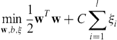
constrained by:
![]()
where ![]() is a nonnegative slack variable for penalizing misclassifications. The function
is a nonnegative slack variable for penalizing misclassifications. The function ![]() that maps data points into the higher dimensional space is not explicitly represented; rather, a kernel function,
that maps data points into the higher dimensional space is not explicitly represented; rather, a kernel function, ![]() , is used to implicitly specify this mapping. In our application, we use the popular radial basis function (RBF) kernel:
, is used to implicitly specify this mapping. In our application, we use the popular radial basis function (RBF) kernel:
![]()
A standard one-vs-one voting scheme is used where all (![]() ) pairwise binary classifiers are trained and the most popular label is selected. Many efficient implementations of SVMs are publicly available; we use LIBSVM [9].
) pairwise binary classifiers are trained and the most popular label is selected. Many efficient implementations of SVMs are publicly available; we use LIBSVM [9].
We train our classifiers using a collection of simulated games in Rush collected under controlled conditions: 40 instances of every possible combination of offense (8) and defense plays (8), from each of the 12 starting formation configurations. Since the starting configuration is known, each series of SVMs is only trained with data that could be observed starting from its given configuration. For each configuration, we create a series of training sequences that accumulates spatiotemporal traces from ![]() up to
up to ![]() timesteps. A multiclass SVM (i.e., a collection of 28 binary SVMs) is trained for each of these training sequence lengths. Although the aggregate number of binary classifiers is large, each classifier only employs a small fraction of the dataset and is therefore efficient (and highly parallelizable). Cross-validation on a training set was used to tune the SVM parameters (
timesteps. A multiclass SVM (i.e., a collection of 28 binary SVMs) is trained for each of these training sequence lengths. Although the aggregate number of binary classifiers is large, each classifier only employs a small fraction of the dataset and is therefore efficient (and highly parallelizable). Cross-validation on a training set was used to tune the SVM parameters (![]() and
and ![]() ) for all of the SVMs.
) for all of the SVMs.
Classification at testing time is very fast and proceeds as follows. We select the multiclass SVM that is relevant to the current starting configuration and timestep. An observation vector of the correct length is generated (this can be done incrementally during game play) and fed to the multiclass SVM. The output of the play recognizer is the system’s best guess (at the current timestep) about the opponent’s choice of defensive play and can help us to select the most appropriate offense, as discussed next.
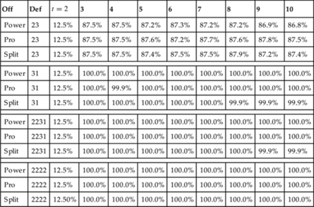
Table 13.1 summarizes the experimental results for different lengths of the observation vector (time from start of play), averaging classification accuracy across all starting formation choices and defense choices. We see that at the earliest timestep, our classification accuracy is at the baseline but jumps sharply to near perfect levels at ![]() . This definitely confirms the feasibility of accurate play recognition in Rush, even during very early stages of a play. At
. This definitely confirms the feasibility of accurate play recognition in Rush, even during very early stages of a play. At ![]() , there is insufficient information to discriminate between offense plays (perceptual aliasing); however, by
, there is insufficient information to discriminate between offense plays (perceptual aliasing); however, by ![]() , the positions of the offensive team are distinctive enough to be reliably recognized.
, the positions of the offensive team are distinctive enough to be reliably recognized.
Table 13.1
Play Recognition Results
Since Rush is a simulated game, it is possible for the play recognizer to perfectly observe the environment, which may be an unrealistic assumption in the real world. To address this, we replicated the experiments under conditions where both training and test data were corrupted by observation noise. We model this noise as a Gaussian with 0 mean and ![]() yard. Figure 13.3 presents a more detailed look at the play-recognition accuracy for each of the 12 starting configurations, both with and without noise. Most of the curves look very similar, but we see that recognition accuracy climbs more slowly for formations where the offense has selected power plays; this occurs because two of the power plays are very similar, differing only in the fullback position.
yard. Figure 13.3 presents a more detailed look at the play-recognition accuracy for each of the 12 starting configurations, both with and without noise. Most of the curves look very similar, but we see that recognition accuracy climbs more slowly for formations where the offense has selected power plays; this occurs because two of the power plays are very similar, differing only in the fullback position.
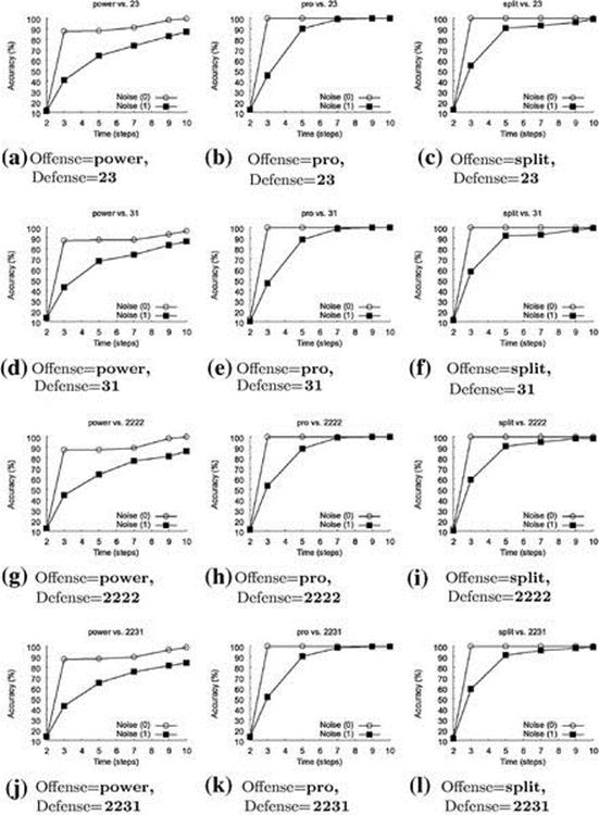
FIGURE 13.3 Classification results versus time, with and without noise for all offensive and defensive formation combinations. Observational noise is modeled on a zero mean Gaussian distribution with ![]() yard. For the no noise condition, there is a sharp jump in accuracy between timesteps 2 and 3, moving from chance accuracy to
yard. For the no noise condition, there is a sharp jump in accuracy between timesteps 2 and 3, moving from chance accuracy to ![]() . Variants of the power offense are the most difficult to identify correctly; the classification is not perfect even at timestep 10 in the presence of noise. Based on these experiments, timestep 3 was selected as the best time for play adaptation, since delaying yields negligible improvements in play recognition for the no noise case.
. Variants of the power offense are the most difficult to identify correctly; the classification is not perfect even at timestep 10 in the presence of noise. Based on these experiments, timestep 3 was selected as the best time for play adaptation, since delaying yields negligible improvements in play recognition for the no noise case.
However, reliably identifying the opponent’s strategy is only one of the challenges that need to be addressed toward the creation of an adaptive football team. In the next section, we discuss the problem of avoiding coordination failures while performing runtime play adaptation.
13.5 Team Coordination
Effective player coordination has been shown to be an important predictor of team success in adversarial games such as Robocup soccer [38]. Much work has centered on the problem of role allocation—correctly allocating players to roles that are appropriate for their capabilities and smoothly transitioning players between roles [35]. In the worst case, determining which players to group together to accomplish a task requires searching over an intractable set of potential team assignments [36]. In many cases there are simple heuristics that can guide subgroup formation; for instance, subgroups often contain agents with diverse capabilities, which limits potential assignments.
We demonstrate a novel method for discovering which agents will make effective subgroups based on an analysis of game data from successful team plays. After extracting the subgroups we implement a supervised learning mechanism to identify the key group of players most critical to each play.
The following are the three general types of cues that can be used for subgroup extraction:
• Spatial—relationships between team members that remain constant over a period of time
• Temporal—co-occurrence of related actions between different team members
• Coordination—dependencies between team members’ actions
Our subgroup extraction method uses all of these to build a candidate set of subgroups. By examining mutual information between the offensive player, defensive blocker, and ball location along with the observed ball workflow, we can determine which players frequently coordinate in previously observed plays. Although automatic subgroup identification could be useful for applications (e.g., opponent modeling or game commentary), in this chapter we show how extracted subgroups can be used to limit the search space when creating new multiagent plays using two play generation methods: (1) play adaptation of existing plays and (2) Monte Carlo search using Upper Confidence bounds applied to Trees (UCT).
The basic idea behind our approach is to identify subgroups of coordinated players by observing a large number of football plays. In our earlier work [23], we demonstrated that appropriately changing the behavior of a critical subgroup (e.g., QB, RB, FB) during an offensive play, in response to a recognized defensive strategy, significantly improves yardage; however, the previous work relied entirely on domain knowledge to identify the key players. In contrast, this work automatically determines the critical subgroups of players (for each play) by an analysis of spatiotemporal observations to determine all subgroups and supervised learning to learn which ones will garner the best results. Once the top-ranked candidate subgroup has been identified, we explore two different techniques for creating new plays: (1) dynamic play adaptation of existing plays and (2) a UCT search.
13.5.1 Automatic Subgroup Detection
To determine which players should be grouped together, we first must understand dependencies among the eight players for each formation. All players coordinate to some extent, but some players’ actions are so tightly coupled that they form a subgroup during the given play. Changing the command for one athlete in a subgroup without adjusting the others causes the play to lose cohesion, potentially resulting in a yardage loss rather than a gain. We identify subgroups using a combination of two methods—the first based on a statistical analysis of player trajectories and the second based on workflow.
The mutual information between two random variables measures their statistical dependence. Inspired by this, our method for identifying subgroups attempts to quantify the degree to which the trajectories of players are coupled, based on a set of observed instances of the given play. However, the naive instantiation of this idea, which simply computes the dependence between player trajectories without considering the game state, is doomed to failure. This is because offensive players’ motions are dominated by three factors: (1) its plan as specified by the playbook, (2) the current position of the ball, and (3) the current position of the defensive player assigned to block a play.
So, if we want to calculate the relationships between the offensive players, we need to place their trajectories in a context that considers these factors. Our method for doing this is straightforward. Rather than computing statistics on raw player trajectories, we derive a feature that includes these factors and compute statistics between the feature vectors as follows.
First, for each player on the offense, we determine the trajectory of the defensive player assigned to block him. Since this assigned defensive player is typically the opponent that remains closest to the player during the course of the play, we determine the assigned defender to be the one whose average distance to the given player is the least. More formally, for a given offensive player, ![]() , the assigned defender,
, the assigned defender, ![]() , is:
, is:
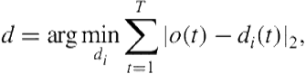 (13.1)
where ![]() and
and ![]() denote the 2D positions of the given players at time
denote the 2D positions of the given players at time ![]() . Our feature
. Our feature ![]() is simply the centroid (average) of
is simply the centroid (average) of ![]() , and the ball position
, and the ball position ![]() :
:
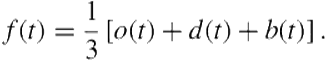 (13.2)
We can now compute sets of features ![]() and
and ![]() from the collection of observed plays for a given pair of offensive players
from the collection of observed plays for a given pair of offensive players ![]() and
and ![]() , treating observations through time simply as independent measurements. We model the distributions
, treating observations through time simply as independent measurements. We model the distributions ![]() and
and ![]() of each of these features as 2D Gaussian distributions with diagonal covariance.
of each of these features as 2D Gaussian distributions with diagonal covariance.
We then quantify the independence between these feature distributions using the symmetricized Kullback-Leibler divergence [21]:
![]() (13.3)
(13.3)
where
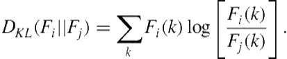 (13.4)
Pairs of athletes with low ![]() are those whose movements during a given play are closely coupled. We compute the average
are those whose movements during a given play are closely coupled. We compute the average ![]() score over all pairs
score over all pairs ![]() in the team and identify as candidate subgroups those pairs with scores that falls in the lowest quartile.Figure 13.4 shows an example of connections detected using this metric.
in the team and identify as candidate subgroups those pairs with scores that falls in the lowest quartile.Figure 13.4 shows an example of connections detected using this metric.
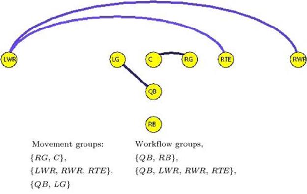
FIGURE 13.4 Connections found by measuring ![]() mutual information in the Pro vs. 23 formations. These links reveal players whose movements during a play are closely coupled. Connected players are organized into a list of movement groups. Workflow groups represent how ball possession is transferred between players during a play. These lists of subgroups are used as candidates for dynamic play adaptation, since modifying the actions of these players is likely to radically influence the play’s outcome. To avoid destroying these interdependencies, the play-adaptation system modifies the actions of these players as a group rather than individually.
mutual information in the Pro vs. 23 formations. These links reveal players whose movements during a play are closely coupled. Connected players are organized into a list of movement groups. Workflow groups represent how ball possession is transferred between players during a play. These lists of subgroups are used as candidates for dynamic play adaptation, since modifying the actions of these players is likely to radically influence the play’s outcome. To avoid destroying these interdependencies, the play-adaptation system modifies the actions of these players as a group rather than individually.
The grouping process involves more than just finding the mutual information (MI) between players. We must also determine relationships formed based on possession of the football. When the QB hands the ball off to the RB or FB their movements are coordinated for only a brief span of time before the ball is transferred to the next player. Because of this, the MI algorithm described before does not adequately capture this relationship. We developed another mechanism to identify such workflows and add them to the list of MI-based groups.
Our characterization of the workflow during a play is based on ball transitions. Given our dataset, we count transitions from one player to another. The historical data indicates that, in almost all offensive formations, the RB receives the ball the majority of the time, lessened only when the FB is in play, in which case we see the ball typically passed from the QB to either the RB or the FB. Consequently, the {QB, RB, and FB} naturally forms a group for running plays, termed a “key group” in Laviers and Sukthankar [23]. The same happens between the QB and the players receiving the ball in passing plays, which forms another workflow group {QB, LWR, RWR, and RTE}. The final list of candidates is therefore simply the union of the MI candidates and the workflow candidates (seeFigure 13.4).
13.5.2 Dynamic Play Adaptation
Figure 13.5 gives an overview of the dynamic play-adaptation system; based on our estimate of the most likely defensive formation sensed early in the play (at time ![]() ), we switch the key subgroup to an existing play that has the best a priori chance of countering the opponent’s strategy (see Figure 13.6). Note that attempting to switch the entire play once execution has started is less effective than adapting the play in a limited manner by only changing the behavior of a key subgroup. As described in Section 13.4, we trained a set of SVMs to recognize defensive plays at a particular time horizon based on observed player trajectories. We rely on these to recognize the opponent’s strategy at an early stage in the play and we identify the strongest counter based on the yardage history of the offensive playbook against the recognized defense. This can be precomputed and stored in a lookup table indexed by the current offensive play and the likely defense.
), we switch the key subgroup to an existing play that has the best a priori chance of countering the opponent’s strategy (see Figure 13.6). Note that attempting to switch the entire play once execution has started is less effective than adapting the play in a limited manner by only changing the behavior of a key subgroup. As described in Section 13.4, we trained a set of SVMs to recognize defensive plays at a particular time horizon based on observed player trajectories. We rely on these to recognize the opponent’s strategy at an early stage in the play and we identify the strongest counter based on the yardage history of the offensive playbook against the recognized defense. This can be precomputed and stored in a lookup table indexed by the current offensive play and the likely defense.
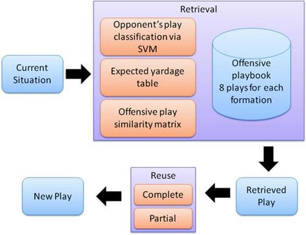
FIGURE 13.5 Overview of the dynamic play adaptation system. Shortly after the start of play, the defensive play is recognized using a set of SVM classifiers. The performance history of the currently executing offensive play versus the recognized defensive play is calculated using the expected yardage table. If it falls below an acceptable threshold, candidate offensive plays for play adaptation are identified using the offensive play similarity matrix. The aim is to find a better performing offensive play that is sufficiently similar to the currently executing one such that the transition can be made without problems. The play-adaptation system can opt for partial reuse (only modifying the actions of a subset of players) or complete reuse (switching all players to the new play).

FIGURE 13.6 Example of dynamic play adaptation. Given an original play (left) and a historically strong counter to the recognized defense (center), we change the behavior of a key subgroup to generate the adapted play (right). The bold (green) line shows the average yardage gained. Note that attempting a complete play switch (center) is inferior to switching the key subgroup (right). (For interpretation of the references to color in this figure legend, the reader is referred to the web version of this book.)
13.6 Offline UCT for Learning Football Plays
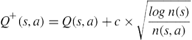
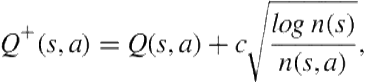
As an alternative to the simple one-time adaptation offered by the play-switch method, we investigated the use of UCT (Upper Confidence bounds applied to Trees) [19], a more powerful policy-generation method that performs Monte Carlo rollouts of the complete game from the current state [22]. Monte Carlo search algorithms have been successfully used in games that have large search spaces [10,8,7,45]. In UCT, an upper confidence bound, ![]() , is calculated for each node in the tree based on the reward history and the number of state visitations. This bound is used to direct the search to the branches most likely to contain the optimal plan; unlike
, is calculated for each node in the tree based on the reward history and the number of state visitations. This bound is used to direct the search to the branches most likely to contain the optimal plan; unlike ![]() pruning, the upper-confidence bound is not used to prune actions. After the rollout budget for a level of the game tree has been exhausted, the action with the highest value of
pruning, the upper-confidence bound is not used to prune actions. After the rollout budget for a level of the game tree has been exhausted, the action with the highest value of ![]() is selected and the search commences at the next level. The output of the algorithm is a policy that governs the movement of the players.
is selected and the search commences at the next level. The output of the algorithm is a policy that governs the movement of the players.
Here we describe a method for creating customized offensive plays designed to work against a specific set of defenses. Using the top-ranked extracted subgroups to focus the investigation of actions yields significant runtime reduction over a standard UCT implementation. To search the complete tree without using our subgroup selection method would require an estimated 50 days of processing time in contrast to the 4 days required by our method.
Offensive plays in the Rush 2008 Football Simulator share the same structure across all formations. Plays typically start with a runTo command, which places a player at a strategic location to execute another play command. After the player arrives at this location, there is a decision point in the play structure where an offensive action can be executed. To effectively use a UCT style exploration we needed to devise a mechanism for combining these actions into a hierarchical tree structure in which the most important choices are decided first.
Because of the potentially prohibitive number of possible location points, we initially search through the possible combinations of offensive high-level commands for the key players, even though chronologically the commands occur later in the play sequence. Once the commands are picked for the players, the system employs binary search to search the runTo area for each of the players—see Figure 13.7(a). The system creates a bounding box around each player’s historical runTo locations, and at Level 2 (immediately after the high-level command is selected), the bounding box is split in half. Following Monte Carlo expansion the location is initially randomly selected. At Level 3 the space is again divided in half and the process continues until Level 5 in Figure 13.7(b), where the player is provided a runTo location, which represents ![]() of the bounding box area. The system takes a sample only at the leaf.
of the bounding box area. The system takes a sample only at the leaf.
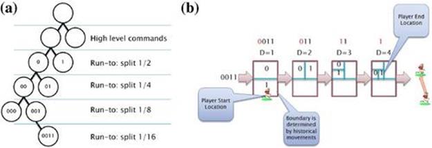
FIGURE 13.7 2D location binary search. (a) A representation of the UCT sparse tree for one player. (b) This graph shows how the binary string generated in the search tree creates a location for a player to move to in the runTo portion of the play.
This 2D search was designed to maintain as small a sampling as possible without harming the system’s chance of finding solutions that produce large yardage gains. To focus the search, the locations each player can move to are bounded to be close (within 1 yard) to the region covered by the specific player in the training data. At the leaf node, the centroid of the square is calculated and the player uses that location to execute the runTo command. Our method effectively allows the most important features to be considered first and the least important last. For comparison, we implemented a similar algorithm that picks random points within the bounding box rather than using the binary split method to search the continuous space of runTo actions.
As mentioned, action modifications are limited to the players in the top-ranked subgroup identified using ![]() ; the other players execute commands from the original play. Our system needs to determine the best plan over a wide range of opponent defensive configurations. To do this, for each rollout the system randomly samples 50% of all possible defenses (evens or odds, one for testing and the other for training) and returns the average yardage gained in the sampling. Since the UCT method provides a ranked search with the most likely solutions grouped near the start of the search, we limit the search algorithm to 2500 rollouts with the expectation that a good solution will be found in this search space.
; the other players execute commands from the original play. Our system needs to determine the best plan over a wide range of opponent defensive configurations. To do this, for each rollout the system randomly samples 50% of all possible defenses (evens or odds, one for testing and the other for training) and returns the average yardage gained in the sampling. Since the UCT method provides a ranked search with the most likely solutions grouped near the start of the search, we limit the search algorithm to 2500 rollouts with the expectation that a good solution will be found in this search space.
We implemented UCT in a distributed system constructed in such a way to prevent multiple threads from sampling the same node. The update function for ![]() was modified to increment the counter after the node is visited but before the leaf is sampled. Since sampling takes close to one second, it is imperative for the exploring threads to know when a node is touched to avoid infinite looping at a node.
was modified to increment the counter after the node is visited but before the leaf is sampled. Since sampling takes close to one second, it is imperative for the exploring threads to know when a node is touched to avoid infinite looping at a node.
After a node is sampled, the update function is called to update ![]() .
.
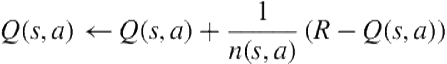 (13.5)
and
 (13.6)
where ![]() is the reward,
is the reward, ![]() is the total number of iterations multiplied by the number of defenses sampled, and
is the total number of iterations multiplied by the number of defenses sampled, and ![]() is the list of yards gained in each sample.
is the list of yards gained in each sample.
Action selection is performed using a variant of the UCT formulation, ![]() , where
, where ![]() is the policy used to choose the best action
is the policy used to choose the best action ![]() from state
from state ![]() . Before revisiting a node, each unexplored node from the same branch must have already been explored; selection of unexplored nodes is accomplished randomly. Using a similar modification to the bandit as suggested in Balla and Fern [4], we adjust the upper confidence calculation
. Before revisiting a node, each unexplored node from the same branch must have already been explored; selection of unexplored nodes is accomplished randomly. Using a similar modification to the bandit as suggested in Balla and Fern [4], we adjust the upper confidence calculation
to employ ![]() , where
, where ![]() for our domain.
for our domain.
We evaluated the efficacy of our method for generating passing plays, which require tightly coupled coordination between multiple players to succeed. Figure 13.8 shows the learning rate for the three proposed search procedures:
Binary Search with Key Groups: Binary search is used to identify runTo locations for the players and the UCT search is conducted for a subgroup of key players. The other players use the commands from the Rush playbook for the specified offensive play.
Random Placement with Key Groups: The runTo location is randomly selected for the players, and UCT search is conducted for a subgroup of key players.
Random Placement, Random Players: We use the random group that performed the best in prior experiments, and the runTo location is randomly selected.
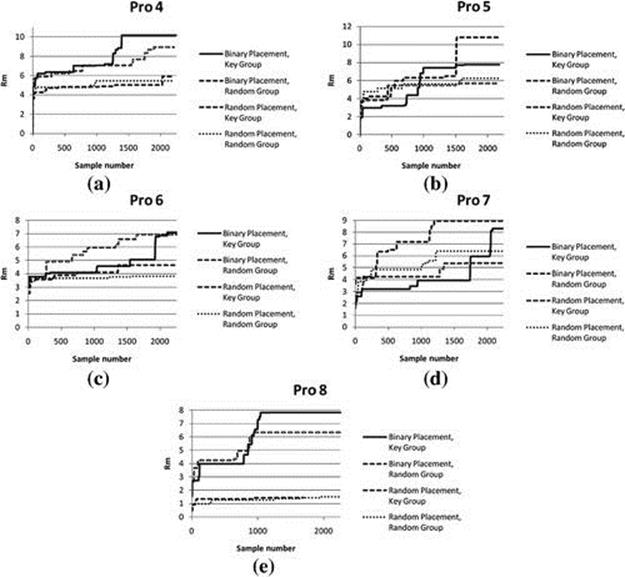
FIGURE 13.8 Binary search with key groups performs the best in most but not all of the cases. Rm is the argmax of the running average of the last ten rewards and represents a good approximation of the expected yardage gained by using the best play at that sample.
Our version of UCT was seeded with Pro formation variants (4–8). Each configuration was run for three days and accumulated 2250 samples (a total of 80 days of CPU time). The ![]() -axis represents the sample number and the
-axis represents the sample number and the ![]() -axis represents
-axis represents ![]() and
and ![]() . All methods perform about equivalently well with a low number of samples, but by 2000 samples, our recommended search method (Binary Search with Key Groups) usually outperforms the other options, particularly when key groups are not employed.
. All methods perform about equivalently well with a low number of samples, but by 2000 samples, our recommended search method (Binary Search with Key Groups) usually outperforms the other options, particularly when key groups are not employed.
Figure 13.9 summarizes experiments comparing UCT (limited by subgroup) against the baseline Rush playbook and play adaptation. Overall, the specialized playbook created offline with UCT consistently outperforms both the baseline Rush system and dynamic play adaptation by several yards. The main flaw with the dynamic play adaptation is that it only modifies the play once in response to the results of the play recognizer. The next section describes an alternative to that approach in which the policy is learned using an online version of UCT and the team continues to adapt in real time.
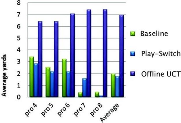
FIGURE 13.9 Comparison of multiagent policy-generation methods starting in the Pro formation. Offline play customization using UCT outperforms the baseline playbook and the play-adaptation method.
13.7 Online UCT for Multiagent Action Selection
Often in continuous-action games the information from plan recognition is used in an ad hoc way to modify the agent’s response, particularly when the agent’s best response is relatively obvious. In this section, we describe how coupling plan recognition with plan repair can be a powerful combination, particularly in multiagent domains where replanning from scratch is difficult to do in real time.
Paradoxically, plan repair can easily get worse over all play performance by causing miscoordinations between players; even minor timing errors can significantly compromise the efficacy of a play. Moreover, it is difficult to predict future play performance at intermediate play-execution stages since effective and ineffective plays share many superficial similarities. This section introduces an approach for learning effective plan repairs using a real-time version of UCT. Data from offline UCT searches is leveraged to learn state and reward estimators capable of making limited predictions of future actions and play outcomes. Our UCT search procedure uses these estimators to calculate successor states and rewards in real time. Experiments show that the plan repairs learned by our method offer significant improvements over the offensive plays executed by the baseline (non-AI system) and also a heuristic-based repair method. Figure 13.10 provides an overview of the key elements of our implementation.
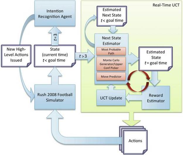
FIGURE 13.10 High-level diagram of our system. To run in real time, our variant of UCT uses a successor state estimator learned from offline traces to calculate the effects of random rollouts. The reward is estimated from the projected terminal state (just before the QB is expected to throw the ball, designated in the diagram as the goal time).
Prior work on UCT for multiagent games has either relied on hand-coded game simulations [4] or use of the actual game to evaluate rollouts (as is done in our offline UCT implementation). In this section, we describe how data from the millions of games run during the offline UCT play generation process can be used to enable online UCT. A similar approach was demonstrated by Gelly and Silver [12] in which the value function used by UCT is learned during offline training. This value function is then used during an online UCT search, significantly improving the search’s performance. Their approach is to initialize ![]() values using previously learned
values using previously learned ![]() and
and ![]() values for each state visited during the offline learning process. Rather than using previously initialized
values for each state visited during the offline learning process. Rather than using previously initialized ![]() values, we learn new
values, we learn new ![]() values but use data from previous games to learn movement predictors and reward estimators.
values but use data from previous games to learn movement predictors and reward estimators.
13.7.1 Method
Each play is segmented into three parts: (1) the time period before the system can determine the defensive play, (2) the period between recognition and the time when the QB throws the ball, and (3) the time between the throw and the end of the play. The proposed system only controls players’ actions in the third segment (Figure 13.11) so that ![]() . Our system for learning plan repairs in real time relies on the following components.
. Our system for learning plan repairs in real time relies on the following components.
Play recognizer: We treat the problem of play recognition as a multiclass classification problem to identify the formation and play variant currently being executed by the defense. Although recognizing the static formation is straightforward, early recognition of play variants is challenging. We achieve 90% accuracy at time ![]() using a multiclass SVM. At
using a multiclass SVM. At ![]() the key players are sent the high-level commands learned in the offline UCT algorithm to perform best for the specific variant in play. The players do not start executing the high-level commands until
the key players are sent the high-level commands learned in the offline UCT algorithm to perform best for the specific variant in play. The players do not start executing the high-level commands until ![]() .
.
Next state estimator: To execute UCT rollouts in real time, our system must predict how defensive players will react as the offense adjusts its play. We train state and reward estimators using offline data from previous UCT searches and employ them in real time.
Reward estimator: To calculate UCT Q-values in the predicted future state, the system estimates reward (yardage) based on relative positions of the players. Because of the inherent stochasticity of the domain, it is difficult to learn a reward estimator early in the play. We focus on estimating yardage at a later stage of the play—just before we expect the QB to throw the ball.
UCT search: Using the state and reward estimators, we use the UCT search algorithm to generate a sparse tree to select actions for the key offensive players, a three-player subset of the team is automatically determined in advance. The search procedure is reexecuted at every timestep to account for unexpected actions taken by the defense.
Rush simulator: The selected player actions are issued to the Rush simulator via network sockets. The simulator returns the new locations of all offensive and defensive players to be used by the estimators.
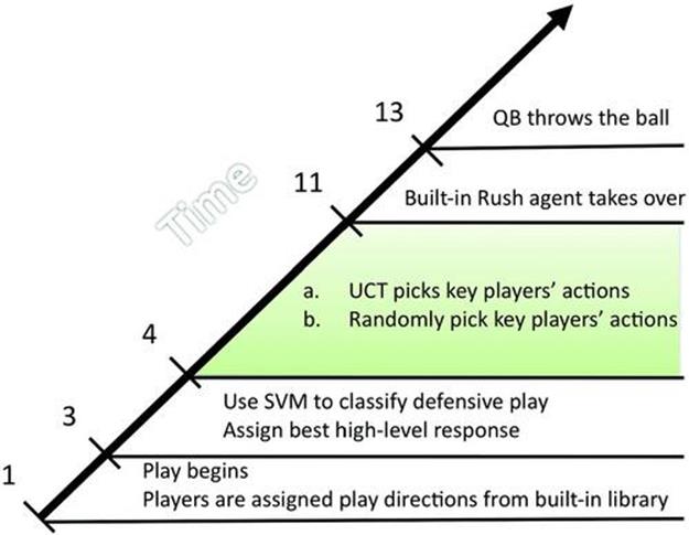
FIGURE 13.11 The timeline of events comprising one play.
13.7.2 UCT Search
After recognizing the play, UCT is employed to search for the best action available to each of the key players (Figure 13.12). Key players are a subset of three offensive players identified offline for a specific formation. As described in Section 13.6, UCT seeks to maximize the upper-confidence bound by preferentially exploring regions with the best probability of producing a high reward. The UCT search is repeatedly called for a predetermined number of rollouts; our real-time implementation sets ![]() , which produced the best results while still allowing real-time execution.
, which produced the best results while still allowing real-time execution.
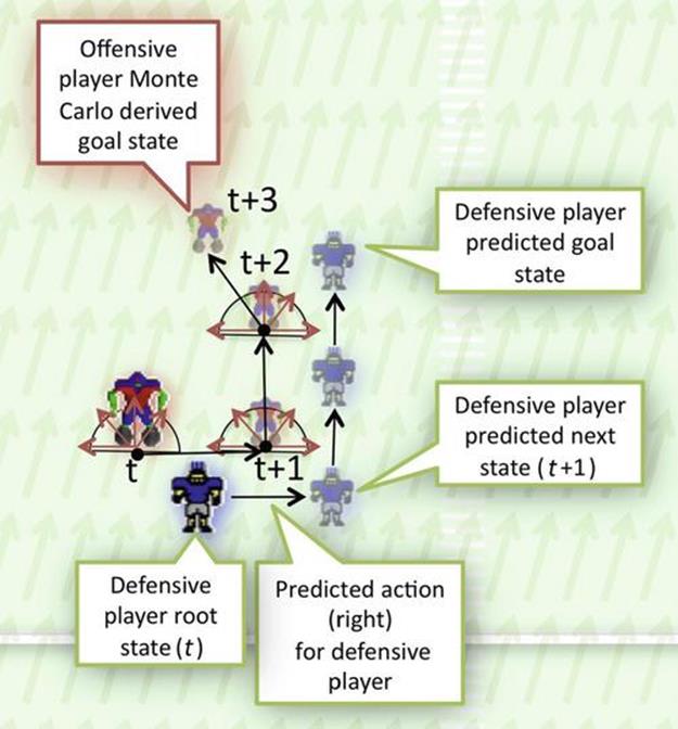
FIGURE 13.12 This image depicts one MC rollout for three timesteps starting at ![]() . The Monte Carlo sparse tree generator determines the action and subsequent next state for the offensive key player and the move predictor uses that action and state information to predict the next action and state for the defensive player. This process is recursively called until the goal state is reached and for all defensive players and their closest offensive players. If the closest offensive player is not a key player, his actions are determined based on the most likely action he took historically.
. The Monte Carlo sparse tree generator determines the action and subsequent next state for the offensive key player and the move predictor uses that action and state information to predict the next action and state for the defensive player. This process is recursively called until the goal state is reached and for all defensive players and their closest offensive players. If the closest offensive player is not a key player, his actions are determined based on the most likely action he took historically.
We define ![]() , where
, where ![]() is in the set of locations of all players as well as the location of the ball. Action
is in the set of locations of all players as well as the location of the ball. Action ![]() contains the combination of actions for key players,
contains the combination of actions for key players, ![]() , where
, where ![]() for a total of eight possible actions.
for a total of eight possible actions.
For the online UCT algorithm, we set the upper-confidence calculation to:
 (13.7)
where ![]() . We tested setting the upper confidence assuming
. We tested setting the upper confidence assuming ![]() , which worked well in our offline UCT play-generation system [22]; unfortunately, this did not work as well in the real-time UCT system. Typically,
, which worked well in our offline UCT play-generation system [22]; unfortunately, this did not work as well in the real-time UCT system. Typically, ![]() is a constant used to tune the biasing sequence to adjust exploration/exploitation of the search space. After extensive empirical evaluation, we found the original UCB1 form worked best. The quality function
is a constant used to tune the biasing sequence to adjust exploration/exploitation of the search space. After extensive empirical evaluation, we found the original UCB1 form worked best. The quality function ![]() , as in Section 13.6, is still the expected value of the node when taking action
, as in Section 13.6, is still the expected value of the node when taking action ![]() from state
from state![]() and ranges from 0 to 1.
and ranges from 0 to 1.
After a node is sampled, the number of times the node is sampled ![]() and
and ![]() is updated. This update occurs recursively from the leaf node to the root node and is the same as the offline UCT implementation. For this spatial-search problem, if actions are explored randomly, players will remain within a small radius of their starting positions. Even in conjunction with UCT, it is unlikely to find a good path. To eliminate circular travel, the system uses an attractive potential field [2] in the direction of the goal that guides exploration toward the correct end zone.
is updated. This update occurs recursively from the leaf node to the root node and is the same as the offline UCT implementation. For this spatial-search problem, if actions are explored randomly, players will remain within a small radius of their starting positions. Even in conjunction with UCT, it is unlikely to find a good path. To eliminate circular travel, the system uses an attractive potential field [2] in the direction of the goal that guides exploration toward the correct end zone.
The path closest to the direction indicated by the potential field is selected as the primary angle. The two neighboring movement directions to the primary angle are also included in the action-search space. Assuming the potential field points up for all key players at ![]() , the expansion of the UCT tree would look like what is shown in Figure 13.13. Also, for every offensive formation, plan repairs are limited to a small subgroup of key players; the remaining players continue executing the original offensive play. The initial configuration of the players governs the players that are most likely to have a decisive impact on the play’s success; by focusing search on a key subgroup of these three players (out of the total team of eight), we speed the search process significantly and concentrate the rollouts on higher expected reward regions. In the results section, we separately evaluate the contribution of these heuristics toward selecting effective plan repairs.
, the expansion of the UCT tree would look like what is shown in Figure 13.13. Also, for every offensive formation, plan repairs are limited to a small subgroup of key players; the remaining players continue executing the original offensive play. The initial configuration of the players governs the players that are most likely to have a decisive impact on the play’s success; by focusing search on a key subgroup of these three players (out of the total team of eight), we speed the search process significantly and concentrate the rollouts on higher expected reward regions. In the results section, we separately evaluate the contribution of these heuristics toward selecting effective plan repairs.
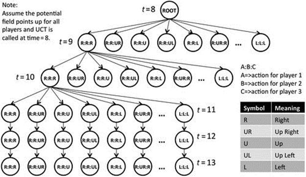
FIGURE 13.13 The real-time UCT expanded out at ![]() . After
. After ![]() the algorithm assumes a straight line until
the algorithm assumes a straight line until ![]() to reduce the state space.
to reduce the state space.
13.7.3 Successor State Estimation
To predict successor states in real time, we perform an incremental determination of where each player on the field could be at the next timestep. To accomplish this update, players are split into three groups: (1) defensive players, (2) offensive key players, and (3) offensive non-key players. The real-time UCT algorithm explores actions by the key players, and the successor state estimator seeks to predict how the defensive players will react to potential plan repairs. Locations of non-key offensive players are determined using the historical observation database to determine the most likely position each non-key offensive player will occupy, given the play variant and timestep. Rather than executing individual movement stride commands, these players are actually performing high-level behaviors built into the Rush simulator; thus, even though these players are technically under our control, we cannot predict with absolute certainty where they will be in the future.
Formally, the game state at time ![]() can be expressed as the vector
can be expressed as the vector
![]() (13.8)
(13.8)
where ![]() , and
, and ![]() denote the
denote the ![]() positions of the offensive and defensive players and the ball, respectively. Similarly, we denote by
positions of the offensive and defensive players and the ball, respectively. Similarly, we denote by ![]() and
and ![]() the actions taken by the offensive player
the actions taken by the offensive player ![]() and defensive player
and defensive player ![]() , respectively, and
, respectively, and ![]() denotes the action of the ball.
denotes the action of the ball.
We predict the actions for the non-key offensive players from the historical archive of previously observed games; we simply advance the play according to the most likely action for each player and adjust the ball state accordingly. However, to determine the actions for the key offensive players (those whose actions will dramatically alter current play), we sample promising actions from the UCT tree using the Monte Carlo rollout. The goal is to alter the current play in a way that improves expected yardage.
Predicting the opponent’s response to the altered play is more difficult. For this, we train a classifier to predict the next action of each defensive player ![]() based on its position and that of its closest offensive player:
based on its position and that of its closest offensive player:
![]() (13.9)
(13.9)
In other words, the classifier learns the mapping:
![]() (13.10)
(13.10)
where ![]() is selected from the discrete set of actions described before. We employ the J.48 classifier from the Weka machine learning toolkit (default parameters) for this purpose. The J.48 classifier is the Weka implementation of the C4.5 algorithm. Applying
is selected from the discrete set of actions described before. We employ the J.48 classifier from the Weka machine learning toolkit (default parameters) for this purpose. The J.48 classifier is the Weka implementation of the C4.5 algorithm. Applying ![]() to the defensive player’s position enables us to predict its future position,
to the defensive player’s position enables us to predict its future position, ![]() . The classifier is trained offline using a set of observed plays and is executed online in real time to predict actions of defensive players.
. The classifier is trained offline using a set of observed plays and is executed online in real time to predict actions of defensive players.
We predict the play state forward up to the time ![]() , where we expect the QB to throw the ball. If by
, where we expect the QB to throw the ball. If by ![]() , the QB has not thrown the ball, we continue predicting for five more timesteps. Table 13.2 shows the confusion matrix for the move predictor trained with 2000 instances and tested using 10-fold cross-validation. Note that this is an example of an unbalanced dataset in which certain actions are extremely rare.
, the QB has not thrown the ball, we continue predicting for five more timesteps. Table 13.2 shows the confusion matrix for the move predictor trained with 2000 instances and tested using 10-fold cross-validation. Note that this is an example of an unbalanced dataset in which certain actions are extremely rare.
Table 13.2
Combined Move Predictor Confusion Matrix
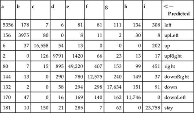
Note: Note that 94.13% were correctly classified.
13.7.4 Reward Estimation
The reward estimator is trained using examples of player configurations immediately preceding the QB throw. At this stage of the play, there is significantly less variability in the outcome than if we attempted to train a reward estimator based on earlier points in the play execution.
The raw training data was unbalanced, containing a disproportionate number of instances with a zero reward. To prevent the reward estimator from being biased toward predicting that none of the configurations will result in a positive reward, we rebalance the training set, discarding many of the samples with zero reward. This procedure helped reward ranges with very few samples to still influence the classifier. We started by finding the average number of instances in each reward bin and then limiting the count of instances to the average value. So if the dataset contained a mean of 100 samples of each value, after collecting 100 zero reward samples, the rest of the zeros in the sample set were discarded.
The reward estimator uses an input vector derived from the game state at the end of the prediction ![]() consisting of a concatenation of the following attributes (Figure 13.14):
consisting of a concatenation of the following attributes (Figure 13.14):
1. ![]() : distance of the QB with the ball to each key offensive player,
: distance of the QB with the ball to each key offensive player, ![]()
2. ![]() : distance from each key offensive player to the scrimmage line
: distance from each key offensive player to the scrimmage line
3. distance from each key offensive player to his closest opponent, ![]()
4. ![]() : the discretized angle from each key offensive player
: the discretized angle from each key offensive player ![]() to his closest opponent
to his closest opponent ![]()
5. sum of the angles traveled for each key offensive player ![]() ,
, ![]()
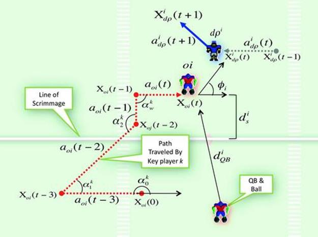
FIGURE 13.14 The features used in the reward classifier. This diagram shows one of the offensive key players ![]() , his closest defensive players
, his closest defensive players ![]() , and the position of the QB holding the ball.
, and the position of the QB holding the ball.
The output is the expected yardage, quantized into seven bins. Our preliminary evaluations indicated that learning a continuous regression model for the yardage was much slower and did not improve accuracy. Therefore, we use the Weka J.48 classifier (default parameters) with the expected yardage treated as a discrete class (0–6). These bins roughly correspond to 10-yard increments (![]() to +50 yards gained per play).
to +50 yards gained per play).
We performed a 10-fold cross-validation to validate the effectiveness of the reward estimator. The estimator was correct in 43% of the instances and close to the correct answer 57% of the time. Since different executions from the same player positions can result in drastically different outcomes, accurately estimating reward is a nontrivial problem. Improving the classification accuracy could potentially improve the effectiveness of our system; however, even with our current reward estimator, the focused UCT search is able to identify promising plan repairs.
In Table 13.3 we show the sum of all the reward confusion matrices. This table highlights weak reward estimation results. Unfortunately, there are a significant number of instances that were classified very high and actually were very low, or classified very low and were actually high. This indicates to us that often there is very little difference in the state between a very successful play and nonsuccessful play. UCT in our case was effective in overcoming this shortfall but would probably benefit from improvement in the reward estimation, whether by a greater number of samples or a revision of the feature set.
Table 13.3
Combined Reward Estimation Confusion Matrix
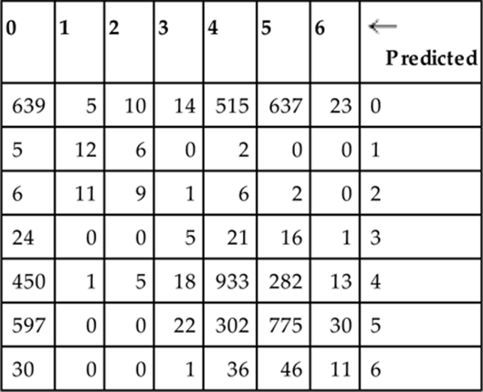
Note: The original yardage rewards are discretized into bins ranging from 0–6. The classifier is correct 43% of the time and is close to correct in 57% of the classified instances. impressively, the online UCT algorithm does a good job of finding good actions even with imperfect reward information.
13.7.5 Results
To demonstrate the effectiveness of the overall system, we compared the plans generated by the proposed method against the unmodified Rush 2008 engine (termed “baseline”) and against a heuristic plan-repair system that selects a legal repair action (with uniform probability) from the available set, using potential field and key player heuristics.
Experiments were conducted using our Rush Analyzer and Test Environment system, shown earlier in Figure 13.1, which we constructed to support experimentation on planning and learning in Rush 2008. Because of the time requirements to connect sockets and perform file operations, RATE operates as a multi-threaded application that increases performance speed by approximately 500%.
Results in Figure 13.15 are shown for the fourth play variant of the Pro formation. This play was selected for testing based on weak baseline results and significant performance improvements with the offline UCT algorithm. To test our results on a variation of possible defensive strategies, we selected 10 of the most effective defensive strategies in which our offense was only able to garner 6.5 yards or less on average in the baseline tests. A two-tailed student t-test reveals that our approach (real-time UCT) outperforms both the baseline and heuristic approaches (![]() ) on total yardage gained.
) on total yardage gained.
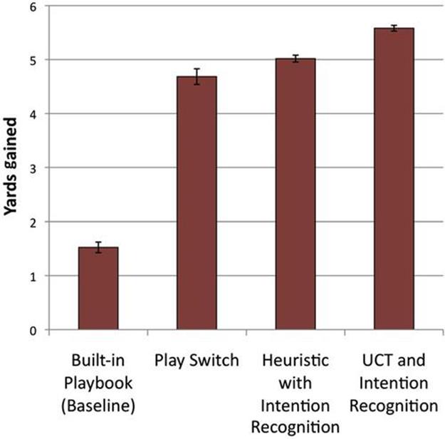
FIGURE 13.15 Relative performance of three systems compared to our real-time UCT algorithm. Note: Error bars mark a 95% confidence interval.
In the baseline test using Rush’s built-in playbook, the selected experimental offense was only able to gain on average 1.5 yards against the selected defensive strategies. Using play recognition and our simple play-switch technique boosts performance by around 3 yards—the most significant performance increase shown. To beat that initial gain, we employ the offline UCT to learn the most effective high-level commands and real-time UCT to boost performance by another yard. In the heuristic with intention recognition condition, the system selects a legal repair action (with uniform probability) from the available set, using the potential field and key player heuristics.
13.8 Conclusion
A missing ingredient in effective opponent modeling for games is the ability to couple plan recognition with plan repair. This chapter describes a real-time method for learning plan repair policies and shows that it is possible to learn successor state and reward estimators from previous searches to do online multiagent Monte Carlo rollouts. Simultaneously predicting the movement trajectories, future reward, and play strategies of multiple players in real time is a daunting task, but we illustrate how it is possible to divide and conquer this problem with an assortment of data-driven game models. Our learned plan repair policies outperform both the baseline system and a simple heuristic-based plan repair method at improving yardage gained on each play execution. More important, our method results in a dramatic drop in the number of interceptions, which is likely to result in significantly longer ball possession periods within the context of a full game. Although the details of the learning process may differ, we believe that our techniques will generalize to other real-time, continuous, multiagent games that lack intermediate reward information (e.g., squad-based shooter games). Like American football, military operations have extensive planning and training phases, with well-rehearsed strategies for ground maneuvers, air battles between fighter jets, and naval encounters. Thus, we believe some aspects of our work will generalize well to military domains.
In future work, we plan to incorporate information about classifier error rates directly into plan repair to enable the calculation of “risk-sensitive” plan repair policies that consider the impact of prediction failures. In this particular domain, our play recognizer classifies plays with a ![]() accuracy, so this feature is not a priority. An unanswered question is the long-term effect of plan repair in computer opponents on player enjoyability. Our hypothesis is that adding plan repair increases the variability of game execution and results in an overall increase in player satisfaction based on the theory espoused by Wray and Laird [46]. However, it is possible that the plan repair algorithm needs to be tuned to provide play at the correct difficulty level rather than simply optimized to be maximally effective; studying the question of adaptive difficulty is an area of future research.
accuracy, so this feature is not a priority. An unanswered question is the long-term effect of plan repair in computer opponents on player enjoyability. Our hypothesis is that adding plan repair increases the variability of game execution and results in an overall increase in player satisfaction based on the theory espoused by Wray and Laird [46]. However, it is possible that the plan repair algorithm needs to be tuned to provide play at the correct difficulty level rather than simply optimized to be maximally effective; studying the question of adaptive difficulty is an area of future research.
References
1. Aler R, Valls J, Camacho D, Lopez A. Programming Robosoccer agents by modeling human behavior. Expert Syst Appl. 2009;36(2, Part 1):1850-1859.
2. Arkin R. Motor schema-based mobile robot navigation. Int J Robot Res. 1989;8(4):92-112.
3. Avrahami-Zilberbrand D, Kaminka G. Fast and complete symbolic plan recognition. Proceedings of International Joint Conference on Artificial Intelligence. 2005:653-658.
4. Balla R, Fern A. UCT for tactical assault planning in real-time strategy games. Proceedings of International Joint Conference on Artificial Intelligence. 2009:40-45.
5. Bhandari I, Colet E, Parker J, Pines Z, Pratap R, Ramanujam K. Advanced scout: data mining and knowledge discovery in NBA data. Data Min Knowl Discov. 1997;1(1):121-125.
6. Camerer C. Behavioral game theory: experiments in strategic interaction. Princeton University Press; 2003.
7. Cazenave T. Nested Monte-Carlo search. Proceedings of International Joint Conference on Artificial Intelligence. 2009:456-461.
8. Cazenave T, Helmstetter B. Combining tactical search and Monte-Carlo in the game of Go. Processings of Computational Intelligene in Games. 2005:171-175.
9. Chang, C, Lin, C. LIBSVM: a library for support vector machines. Software available at <www.csie.ntu.edu.tw/cjlin/libsvm>![]() ; 2001.
; 2001.
10. Chung M, Buro M, Schaeffer J. Monte Carlo planning in RTS games. Proceedings of the IEEE International Conference on Computational Intelligence in Games. 2005.
11. Doshi P, Qu X, Goode A. Decision-theoretic planning in multiagent settings with application to modeling human strategic behavior. In: Sukthankar G, Goldman RP, Geib C, Pynadath DV, Bui HH, eds. Plan, activity, and intent recognition. Waltham, MA: Morgan Kaufmann Publishers; 2014:205-226.
12. Gelly S, Silver D. Combining online and offline knowledge in UCT. Proceedings of the International Conference of Machine Learning. 2007:273-280.
13. Genter K, Agmon N, Stone P. Role-based ad hoc teamwork. In: Sukthankar G, Goldman RP, Geib C, Pynadath DV, Bui HH, eds. Plan, activity, and intent recognition. Waltham, MA: Morgan Kaufmann Publishers; 2014:251-272.
14. Hess R, Fern A, Mortensen E. Mixture-of-parts pictorial structures for objects with variable part sets. Proceedings of International Conference on Computer Vision. 2007:1-8.
15. Intille S, Bobick A. A framework for recognizing multi-agent action from visual evidence. Proceedings of National Conference on Artificial Intelligence. 1999:518-525.
16. Jug M, Pers J, Dezman B, Kovacic S. Trajectory based assessment of coordinated human activity. Proceedings of the International Conference on Computer Vision Systems. 2003:534-543.
17. Kabanza F, Bellefeuille P, Bisson F, Benaskeur A, Irandoust H. Opponent behaviour recognition for real-time strategy games. Proceedings of the AAAI Workshop on Plan, Activity, and Intent Recognition. 2010.
18. Kang Y, Lim J, Kankanhalli M, Xu C, Tian Q. Goal detection in soccer video using audio/visual keywords. International Conference on Information Processing. 2004:1629-1632.
19. Kocsis L, Szepesvari C. Bandit based Monte-Carlo planning. European Conference on Machine Learning. Springer; 2006:282-293.
20. Kuhlmann G, Knox W, Stone P. Know thine enemy: a champion RoboCup coach agent. Proceedings of National Conference on Artificial Intelligence. 2006:1463-1468.
21. Kullback S, Leibler R. On information and sufficiency. Ann Math Statist. 1951;22(1):79-86.
22. Laviers K, Sukthankar G. A Monte Carlo approach for football play generation. Proceedings of Artificial Intelligence for Interactive Digital Entertainment Conference. 2010:150-155.
23. Laviers K, Sukthankar G, Molineaux M, Aha D. Improving offensive performance through opponent modeling. Proceedings of Artificial Intelligence for Interactive Digital Entertainment Conference. 2009:58-63.
24. Li N, Stracuzzi D, Cleveland G, Langley P, Konik T, Shapiro D. Constructing game agents from video of human behavior. Proceedings of Conference on Artificial Intelligence and Interactive Digital Entertainment. 2009:64-69.
25. McCarthy J, Hayes P. Some philosophical problems from the standpoint of artificial intelligence. Machine intelligence. Edinburgh University Press; 1969:463-502.
26. Molineaux, M. Working specification for Rush 2008 interface. Technical Report Knexus Research Corp. May 2008.
27. Molineaux M, Aha D, Sukthankar G. Beating the defense: using plan recognition to inform learning agents. Proceedings of Florida Artificial Intelligence Research Society. 2009:337-342.
28. Nair R, Tambe M, Marsella S, Raines T. Automated assistants for analyzing team behaviors. J Automat Agents Multi-agent Syst. 2004;8(1):69-111.
29. Nichols J, Claypool M. The effects of latency on online Madden NFL football. Proceedings of the International Workshop on Network and Operating Systems Support for Digital Audio and Video. 2004:146-151.
30. Pallavi V, Mukherjee J, Majumdar A, Sural S. Ball detection from broadcast soccer videos using static and dynamic features. J Vis Commun Image Represent. October 2008;19(7):426-436.
31. Riley P, Veloso M. On behavior classification in adversarial environments. In: Parker L, Bekey G, Barhen J, eds. Distributed Autonomous Robotic Systems 4. Springer-Verlag; 2000:371-380.
32. Riley P, Veloso M. Recognizing probabilistic opponent movement models. In: Birk A, Coradeschi S, Tadorokoro S, eds. RoboCup-2001: robot soccer world cup V. Springer-Verlag; 2002:453-458.
33. Riley P, Veloso M, Kaminka G. An empirical study of coaching. In: Asama H, Arai T, Fukuda T, Hasegawa T, eds. Distributed autonomous robotic systems 5. Springer-Verlag; 2002:215-224.
34. Smart Football. How do NFL players memorize all those plays? <http://smartfootball.com/grab-bag/how-do-nfl-players-memorize-all-those-plays>![]() ; 2011.
; 2011.
35. Stone P, Veloso M. Task decomposition, dynamic role assignment, and low-bandwidth communication for real-time strategic teamwork. Artif Intell. 1999;12:241-273.
36. Sukthankar G, Sycara K. Simultaneous team assignment and behavior recognition from spatio-temporal agent traces. Proceedings of National Conference on Artificial Intelligence. July 2006:716-721.
37. Sukthankar G, Sycara K. Policy recognition for multi-player tactical scenarios. Proceedings of International Conference on Autonomous Agents and Multi-Agent Systems. May 2007:59-65.
38. Tambe M. Towards flexible teamwork. J Artif Intell Res. 1997;7:83-124.
39. Tanaka K, Nakashima H, Noda I, Hasida K. Mike: an automatic commentary system for soccer. Proceedings of the International Conference on Multi-Agent Systems. 1998:285-292.
40. Tanaka-Ishii K, Frank I, Arai K. Trying to understand Robocup. AI Mag. 2000;21(3):19-24.
41. USA Football. Let’s talk football: how many plays should a playbook hold? <http://usafootball.com/news/coaches/lets-talk-football-how-many-plays-should-playbook-hold>![]() .
.
42. vanden Herik J, Donkers J, Spronck P. Opponent modeling and commercial games. Procceedings of the Symposium on Computational Intelligence and Games. 2005:15-25.
43. Vapnik V. Statistical learning theory. Wiley & Sons Inc; 1998.
44. Voelz D, Andre E, Herzog G, Rist T. Rocco: a RoboCup soccer commentator system. In: Asada M, Kitano H, eds. RoboCup-98: robot soccer world cup II. Springer; 1999:50-60.
45. Ward CD, Cowling PI. Monte Carlo search applied to card selection in Magic: The Gathering. Proceedings of Computational Intelligence and Games. 2009:9-16.
46. Wray R, Laird J. Variability in human behavior modeling for military simulations. Proceedings of Behavior Representation in Modeling and Simulation Conference. 2003:176-185.
47. Yahoo! Answers. Football playbook: how many plays are usually in one? <http://answers.yahoo.com/question/index?qid=20080725053139AAX9wD7>![]() ; 2008.
; 2008.
All materials on the site are licensed Creative Commons Attribution-Sharealike 3.0 Unported CC BY-SA 3.0 & GNU Free Documentation License (GFDL)
If you are the copyright holder of any material contained on our site and intend to remove it, please contact our site administrator for approval.
© 2016-2026 All site design rights belong to S.Y.A.