Plan, Activity, and Intent Recognition: Theory and Practice, FIRST EDITION (2014)

Part I. Plan and Goal Recognition

Chapter 3. Plan Recognition Using Statistical-Relational Models

Sindhu Raghavan^a, Parag Singla^b and Raymond J. Mooney^a, ^aUniversity of Texas at Austin, Austin, TX, USA, ^bIndian Institute of Technology Delhi, Hauz Khas, DL, India

Abstract

Plan recognition is the task of predicting an agent’s top-level plans based on its observed actions. It is an abductive-reasoning task that involves inferring plans that best explain observed actions. Most existing approaches to plan-recognition and other abductive-reasoning tasks either use first-order logic (or subsets of it) or probabilistic graphical models. While the former cannot handle uncertainty in the data, the latter cannot handle structured representations. To overcome these limitations, we explore the application of statistical–relational models that combine the strengths of both first-order logic and probabilistic graphical models to plan recognition. Specifically, we introduce two new approaches to abductive plan recognition using Bayesian logic programs (BLPs) and Markov Logic Networks (MLNs). Neither of these formalisms is suited for abductive reasoning because of the deductive nature of the underlying logical inference. In this chapter, we propose approaches to adapt both these formalisms for abductive plan recognition. We present an extensive evaluation of our approaches on three benchmark datasets on plan recognition, comparing them with existing state-of-the-art methods.

Keywords

Plan recognition

abduction

reasoning about actions

probabilistic reasoning

statistical–relational learning

Bayesian logic programs

Markov Logic Networks

machine learning

Acknowledgments

We would like to thank Nate Blaylock for sharing the Linux and Monroe datasets and Vibhav Gogate for helping us modify SampleSearch for our experiments. We would also like to thank Luc De Raedt and Angelika Kimmig for their help in our attempt to run ProbLog on our plan-recognition datasets. This research was funded by MURI ARO Grant W911NF-08-1-0242 and U.S. Air Force Contract FA8750-09-C-0172 under the DARPA Machine Reading Program. Experiments were run on the Mastodon Cluster, provided by NSF Grant EIA-0303609. All views expressed are solely those of the authors and do not necessarily reflect the opinions of ARO, DARPA, NSF, or any other government agency.

3.1 Introduction

Plan recognition is the task of predicting an agent’s top-level plans based on its observed actions. It is an abductive-reasoning task that involves inferring cause from effect [11]. Early approaches to plan recognition were based on first-order logic in which a knowledge base (KB) of plans and actions is developed for the domain and then default reasoning [31,30] or logical abduction [45] is used to predict the best plan based on the observed actions. Kautz and Allen [31] and Kautz [30] developed one of the first logical formalizations of plan recognition. They used nonmonotonic deductive inference to predict plans using observed actions, an action taxonomy, and a set of commonsense rules or constraints. The approach of Lesh and Etzioni [41] to goal recognition constructs a graph of goals, actions, and their schemas and prunes the network until the plans present in the network are consistent with the observed goals. The approach by Hong [21] also constructs a “goal graph” and analyzes the graph to identify goals consistent with observed actions. However, these approaches are unable to handle uncertainty in observations or background knowledge and are incapable of estimating the likelihood of different plans.

Another approach to plan recognition is to directly use probabilistic methods. Albrecht et al. [1] developed an approach based on dynamic Bayesian networks (DBN) to predict plans in an adventure game. Horvitz and Paek [22] developed an approach that uses Bayesian networks to recognize goals in an automated conversation system. Pynadath and Wellman [53] extended probabilistic context-free grammars to plan recognition. Kaminka et al. [28] developed an approach to multiagent plan recognition (MAPR) using DBNs to perform monitoring in distributed systems. Bui et al. [6] and Bui [5] used abstract hidden Markov models for hierarchical goal recognition. Saria and Mahadevan [59] extended the work by Bui [5] to MAPR. Blaylock and Allen [2] used statistical -gram models for the task of instantiated goal recognition. Even though these approaches can handle uncertainty and can be trained effectively, they cannot handle the kind of structured relational data that can be represented in first-order predicate logic. Furthermore, it is difficult to incorporate planning domain knowledge in these approaches.

The third category of approaches use aspects of both logical and probabilistic reasoning. Hobbs et al. [20] attach weights or costs to predicates in the knowledge base and use these weights to guide the search for the best explanation. Goldman et al. [19] use the probabilistic Horn abduction [50] framework described by Poole to find the best set of plans that explain the observed actions. Several other approaches use Bayesian networks [9,8,23] to perform abductive inference. Based on the observed actions and a KB constructed for planning, Bayesian networks are automatically constructed using knowledge base model construction (KBMC) procedures. However, most of these approaches do not have the capabilities for learning the structure or the parameters. Another chapter by Inoue et al. [26] in this book explores the use of weighted abduction for large-scale discourse processing.

The last decade has seen a rapid growth in the area of statistical–relational learning (SRL) (e.g., see Getoor and Taskar [16]), which uses well-founded probabilistic methods while maintaining the representational power of first-order logic. Since these models combine the strengths of both first-order logic and probabilistic graphical models, we believe that they are well suited for solving problems like plan recognition. In this chapter, we explore the efficacy of different SRL models for the task of plan recognition. We focus on extending two specific SRL models—Markov Logic Networks (MLNs) [14], based on undirected probabilistic graphical models, and Bayesian logic programs (BLPs) [32], based on directed probabilistic graphical models—to the task of plan recognition.

MLNs attach real-valued weights to formulas in first-order logic in order to represent their certainty. They effectively use logic as a compact template for representing large, complex ground Markov networks. Since MLNs have been shown to formally subsume many other SRL models and have been successfully applied to many problems [14], we chose to explore their application to plan recognition. However, the representational power and flexibility offered by MLNs come at a cost in computational complexity. In particular, many problems result in exponentially large ground Markov networks, making learning and inference intractable in the general case.

Pearl [48] argued that causal relationships and abductive reasoning from effect to cause are best captured using directed graphical models (Bayesian networks). Since plan recognition is abductive in nature, this suggested that we also explore a formalism based on directed models. Therefore, we explored the application of BLPs, which combine first-order Horn logic and directed graphical models, to plan recognition. BLPs use SLD resolution to generate proof trees, which are then used to construct a ground Bayesian network for a given query. This approach to network construction is called knowledge base model construction. Similar to BLPs, prior approaches (i.e., Wellman et al. [66] and Ngo and Haddawy [46]) also employ the KBMC technique to construct ground Bayesian networks for inference.

Another approach, known as probabilistic Horn abduction (PHA) [50], performs abductive reasoning using first-order knowledge bases and Bayesian networks. However, since the BLP framework imposes fewer constraints on representation, both with respect to structure and parameters [33], and since it provides an integrated framework for both learning and inference, we decided to use BLPs as opposed to PHA or other similar formalisms.

Logical approaches to plan recognition, for example, those proposed by Kautz and Allen [31] and Ng and Mooney [45], typically assume a KB of plans and/or actions appropriate for planning, but not specifically designed for plan recognition. The advantage of this approach is that a single knowledge base is sufficient for both automated planning and plan recognition. Also, knowledge of plans and actions sufficient for planning is usually easier to develop than a knowledge base especially designed for plan recognition, which requires specific rules of the form: “If an agent performs action A, they may be executing plan P.” Sadilek and Kautz’s recent MLN-based approach to plan/activity recognition [58,57] requires such manually provided plan-recognition rules.

Our goal is to develop general-purpose SRL-based plan-recognition systems that only require the developer to provide a knowledge base of actions and plans sufficient for planning, without the need to engineer a KB specifically designed for plan recognition. Plan recognition using only planning knowledge generally requires abductive logical inference. BLPs use purely deductive logical inference as a preprocessing step to the full-blown probabilistic inference. Encoding planning knowledge directly into MLNs does not support abductive reasoning either. Further, using the standard semantics of MLNs of grounding the whole theory leads to a blowup for plan-recognition problems. Consequently, neither BLPs nor MLNs can be directly used in their current form for abductive plan recognition.

Therefore, this chapter describes reencoding strategies (for MLNs) as well as enhancements to both models that allow them to use logical abduction. Our other goal involves developing systems capable of learning the necessary parameters automatically from data. Since both BLPs and MLNs provide algorithms for learning both the structure and the parameters, we adapt them in our work to develop trainable systems for plan recognition. The main contributions of this chapter are as follows:

• Adapt SRL models, such as BLPs and MLNs, to plan recognition

• Introduce Bayesian Abductive Logic Programs (BALPs), an adaptation of BLPs that uses logical abduction

• Propose reencoding strategies for facilitating abductive reasoning in MLNs

• Introduce abductive Markov logic, an adaptation of MLNs that combines reencoding strategies with logical abduction to construct the ground Markov network

• Experimentally evaluate the relative performance of BALPs, abductive MLNs (i.e., using reencoding strategies and abductive model construction), traditional MLNs, and existing methods on three plan-recognition benchmarks

The rest of the chapter is organized as follows. First, we provide some background on logical abduction, BLPs, and MLNs in Section 3.2. Section 3.3 presents our extensions to both BLPs and MLNs to include logical abduction. Finally, we present an extensive evaluation of our approaches on three benchmark datasets for plan recognition, comparing them with the existing state-of-the-art for plan recognition, in Section 3.4.

3.2 Background

3.2.1 Logical Abduction

In a logical framework, abduction is usually defined as follows, according to Pople [52], Levesque [42], and Kakas et al. [27]:

Given: Background knowledge and observations , both represented as sets of formulae in first-order logic, where is typically restricted to Horn clauses and to ground literals

Find: A hypothesis , also a set of logical formulae (typically ground literals), such that and

Here, represents logical entailment and represents false; that is, find a set of assumptions consistent with the background theory and explains the observations. There are generally many hypotheses that explain a given set of observations . Following Occam’s Razor, the best hypothesis is typically defined as the one that minimizes the number of assumptions, . Given a set of observations , the set of abductive proof trees is computed by recursively backchaining on each until every literal in the proof is either proved or assumed. Logical abduction has been applied to tasks such as plan recognition and diagnosis by Ng and Mooney [45] and Peng and Reggia [49].

3.2.2 Bayesian Logic Programs

Bayesian logic programs (BLPs) [32] can be viewed as templates for constructing directed graphical models (Bayes nets). Given a knowledge base as a special kind of logic program, standard backward-chaining logical deduction (SLD resolution) is used to automatically construct a Bayes net on the same lines as KBMC (see, for example, Wellman et al. [66] and Breese et al. [4]). More specifically, given a set of facts and a query, all possible Horn-clause proofs of the query are constructed and used to build a Bayes net for answering the query. Standard probabilistic inference techniques are then used to compute the most probable answer.

More formally, a BLP consists of a set of Bayesian clauses, definite clauses of the form , where and are Bayesian predicates (defined in the next paragraph). is called the head of the clause () and () is the body (). When , a Bayesian clause is a fact. Each Bayesian clause is assumed to be universally quantified and range-restricted (i.e., ) and has an associated conditional probability distribution: .

A Bayesian predicate is a predicate with a finite domain, and each ground atom for a Bayesian predicate represents a random variable. Associated with each Bayesian predicate is a combining rule, such as noisy-or or noisy-and, that maps a finite set of s into a single [48]. Let be a Bayesian predicate defined by two Bayesian clauses, and , where and are their cpds. Let be a substitution that satisfies both clauses. Then, in the constructed Bayes net, directed edges are added from the nodes for each and to the node for . The combining rule for is used to construct a single cpd for from and . The probability of a joint assignment of truth values to the final set of ground propositions is then defined in the standard way for a Bayes net: , where represents the set of random variables in the network and represents the parents of .

Once a ground network is constructed, standard probabilistic inference methods can be used to answer various types of queries, as noted in Koller and Friedman [40]. Typically, we would like to compute the most probable explanation (MPE), which finds the joint assignment of values to unobserved nodes in the network that maximizes the posterior probability given the values of a set of observed nodes. This type of inference is also known as the Maximum a posteriori (MAP) assignment and may be used interchangeably in this book. We would also like to compute the marginal probabilities for the unobserved nodes given the values of observed nodes. The combining-rule parameters and cpd entries for a BLP can be learned automatically from data using techniques proposed by Kersting and De Raedt [34].

3.2.3 Markov Logic Networks

Markov logic (e.g., see Richardson and Domingos [55] and Domingos and Lowd [14]) is a framework for combining first-order logic and undirected probabilistic graphical models (Markov networks). A traditional first-order KB can be seen as a set of hard constraints on the set of possible worlds: if a world violates even one formula, its probability is 0. To soften these constraints, Markov logic attaches a weight to each formula in the knowledge base. A formula’s weight reflects how strong a constraint it imposes on the set of possible worlds. Formally, an MLN is a set of pairs , where is a first-order formula and is a real number. A hard clause has an infinite weight and acts as a logical constraint; otherwise, it is a soft clause. Given a set of constants, an MLN defines a ground Markov network with a node in the network for each ground atom and a feature for each ground clause.

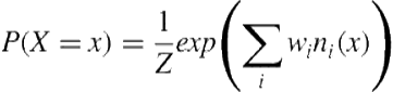
The joint probability distribution over a set of Boolean variables, , corresponding to the nodes in the ground Markov network (i.e., ground atoms) is defined as:

(3.1)

where is the number of true groundings of in and is a normalization term obtained by summing over all values of . Therefore, a possible world becomes exponentially less likely as the total weight of the ground clauses it violates increases.

An MLN can be viewed as a set of templates for constructing ground Markov networks. Different sets of constants produce different Markov networks; however, there are certain regularities in their structure and parameters determined by the underlying first-order theory. Like in BLPs, once the ground network is constructed, standard probabilistic inference methods (i.e., MPE or marginal inference) can be used to answer queries. MLN weights can be learned by maximizing the conditional log-likelihood of training data supplied in the form of a database of true ground literals. A number of efficient inference and learning algorithms that exploit the structure of the network have also been proposed. Domingos and Lowd provide details on these and many other aspects of MLNs [14].

3.3 Adapting Bayesian Logic Programs

Bayesian Abductive Logic Programs are an adaptation of BLPs. In plan recognition, the known facts are insufficient to support the derivation of deductive proof trees for the requisite queries. By using abduction, missing literals can be assumed in order to complete the proof trees needed to determine the structure of the ground network. We first describe the abductive inference procedure used in BALPs. Next, we describe how probabilistic parameters are specified and how probabilistic inference is performed. Finally, we discuss how parameters can be automatically learned from data.

3.3.1 Logical Abduction

Let be the set of observations. We derive a set of most-specific abductive proof trees for these observations using the method originally proposed by Stickel [65]. The abductive proofs for each observation literal are computed by backchaining on each until every literal in the proof is proved or assumed. A literal is said to be proved if it unifies with some fact or the head of some rule in the knowledge base; otherwise, it is said to be assumed. Since multiple plans/actions could generate the same observation, an observation literal could unify with the head of multiple rules in the KB. For such a literal, we compute alternative abductive proofs for each such rule. The resulting abductive proof trees are then used to build the structure of the Bayes net using the standard approach for BLPs.

The basic algorithm to construct abductive proofs is given in Algorithm 3.1. The algorithm takes as input a knowledge base in the form of Horn clauses and a set of observations as ground facts. It outputs a set of abductive proof trees by performing logical abduction on the observations. These proof trees are then used to construct the Bayesian network. For each observation , AbductionBALP searches for rules with consequents that unify with . For each such rule, it computes the substitution from the unification process and substitutes variables in the body of the rule with bindings from the substitution. The literals in the body now become new subgoals in the inference process. If these new subgoals cannot be proved (i.e., if they cannot unify with existing facts or with the consequent of any rule in the KB), then they are assumed. To minimize the number of assumptions, the assumed literals are first matched with existing assumptions. If no such assumption exists, then any unbound variables in the literal that are existentially quantified are replaced by Skolem constants.

Algorithm 3.1 AbductionBALP

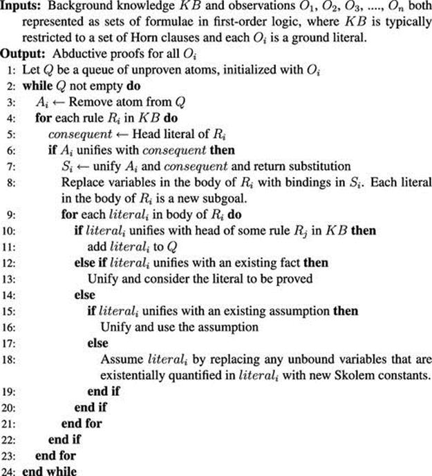
In SLD resolution, which is used in BLPs, if any subgoal literal cannot be proved, the proof fails. However, in BALPs, we assume such literals and allow proofs to proceed until completion. Note that there could be multiple existing assumptions that could unify with subgoals in Step 15. However, if we used all ground assumptions that could unify with a literal, then the size of the ground network would grow exponentially, making probabilistic inference intractable. To limit the size of the ground network, we unify subgoals with assumptions in a greedy manner (i.e., when multiple assumptions match a subgoal, we randomly pick one of them and do not pursue the others). We found that this approach worked well for our plan-recognition benchmarks. For other tasks, domain-specific heuristics could potentially be used to reduce the size of the network.

We now illustrate the abductive inference process with a simple example motivated by one of our evaluation benchmarks, the emergency response domain introduced by Blaylock and Allen [2] in the Monroe dataset described in Section 3.5.1. Consider the partial knowledge base and set of observations given in Figure 3.1(a) and Figure 3.1(b) respectively. The knowledge base consists of rules that give two explanations for a road being blocked at a location: (1) there has been heavy snow resulting in hazardous driving conditions and (2) there has been an accident and the crew is clearing the wreck. Given the observation that a road is blocked, the plan-recognition task involves abductively inferring one of these causes as the explanation.

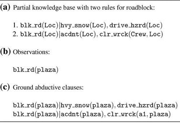
FIGURE 3.1 Partial knowledge base and a set of observations. (a) A partial knowledge base from the emergency response domain in the Monroe dataset. All variables start with uppercase and constants with lowercase. (b) The logical representation of the observations. (c) The set of ground rules obtained from logical abduction.

For each observation literal in Figure 3.1(b), we recursively backchain to generate abductive proof trees. In the given example, we observe that the road is blocked at the location . When we backchain on the literal blk_rd(plaza) using Rule 1, we obtain the subgoals hvy_snow(plaza) and drive_hzrd(plaza). These subgoals become assumptions since no observations or heads of clauses unify them. We then backchain on the literal blk_rd(plaza) using Rule 2 to obtain subgoals acdnt(plaza) and clr_wrk(Crew,plaza). Here again, we find that these subgoals have to be assumed since there are no facts or heads of clauses that unify them. We further notice that clr_wrk(Crew,plaza) is not a fully ground instance. Since is an existentially quantified variable, we replace it with a Skolem constant, , to get the ground assumption clr_wrk(a1,plaza).

Figure 3.1(c) gives the final set of ground rules generated by abductive inference. After generating all abductive proofs for all observation literals, we construct a Bayesian network. Figure 3.2 shows the network constructed for the example in Figure 3.1. Note that since there are no observations and/or facts that unify the subgoals (i.e., hvy_snow(plaza), drive_hzrd(plaza), acdnt(plaza), and clr_wrk(Crew,plaza)) generated during backchaining on observations, SLD resolution will fail to generate proofs. This is typical in plan recognition, and as a result, we cannot use BLPs for such tasks.

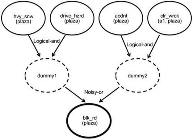
FIGURE 3.2 Bayesian network constructed for the example in Figure 3.1. Note: The nodes with bold borders represent observed actions, the nodes with dotted borders represent intermediate ones used to combine the conjuncts in the body of a clause, and the nodes with thin borders represent plan literals.

3.3.2 Probabilistic Modeling, Inference, and Learning

The only difference between BALPs and BLPs lies in the logical inference procedure used to construct proofs. Once abductive proofs are generated, BALPs use the same procedure as BLPs to construct the Bayesian network. Further, techniques developed for BLPs for learning parameters can also be used for BALPs.

We now discuss how parameters are specified in BALPs. We use noisy/logical-and and noisy-or models to specify the s in the ground Bayesian network because these models compactly encode the with fewer parameters (i.e., just one parameter for each parent node). Depending on the domain, we use either a strict logical-and or a softer noisy-and model to specify the for combining evidence from the conjuncts in the body of a clause. We use a noisy-or model to specify the for combining the disjunctive contributions from different ground clauses with the same head.

Figure 3.2 shows the logical-and and noisy-or nodes in the Bayesian network constructed for the example in Figure 3.1. Given the constructed Bayesian network and a set of observations, we determine the best explanation using the MPE inference [48]. We compute multiple alternative explanations using Nilsson’s k-MPE algorithm [47], as implemented in the ELVIRA Elvira-Consortium [15] package.

Learning can be used to automatically set the noisy-or and noisy-and parameters in the model. In supervised training data for plan recognition, one typically has evidence for the observed actions and the top-level plans. However, we usually do not have evidence for network nodes corresponding to subgoals, noisy-ors, and noisy/logical-ands. As a result, there are a number of variables in the ground networks that are always hidden; thus, expectation-maximization (EM) is appropriate for learning the requisite parameters from the partially observed training data. We use the EM algorithm adapted for BLPs by Kersting and De Raedt [34]. We simplify the problem by learning only noisy-or parameters and using a deterministic logical-and model to combine evidence from the conjuncts in the body of a clause.

3.4 Adapting Markov Logic

As previously mentioned, encoding planning knowledge directly in MLNs does not support abductive reasoning. This is because of the deductive nature of the rules encoding the planning knowledge. In MLNs, the probability of a possible world increases with the total weight of the satisfied formulae. Since an implication is satisfied whenever its consequent is true, an MLN is unable to abductively infer the antecedent of a rule from its consequent. Given the rule and the observation that is true, we would like to abduce as a possible cause for . Since the consequent is true, the clause is trivially satisfied, independent of the value of the antecedent (), and thus does not give any information about the truth value of the antecedent .

This section describes three key ideas for adapting MLNs with logical abductive reasoning, each one building on the previous. First, we describe the Pairwise Constraint (PC) model proposed by Kate and Mooney [29]. Next, we introduce the Hidden Cause (HC) model, which resolves some of the inefficiencies of the PC model. These two models offer strategies for the reencoding MLN rules but do not change the semantics of the traditional MLNs of Richardson and Domingos [55]. Next, we introduce an abductive model-construction procedure on top of the HC model that results in even simpler Markov networks. This gives us the formulation for abductive Markov logic. Our ground Markov network construction strategy is different from the one used in traditional MLNs; thus, our formulation results in different semantics.

We also describe an alternate approach to plan recognition in which the structure of the MLN is manually encoded to enable deductive inference of the top-level plans from observed actions. This allows us to compare abductive Markov logic to a manually encoded MLN for plan recognition.

3.4.1 Pairwise Constraint Model

Kate and Mooney [29] were the first to develop an approach to reencode MLNs with logical abductive reasoning, which we call the Pairwise Constraint model. We describe this approach here since it provides the context for understanding the more sophisticated models introduced in subsequent sections. The key idea is to introduce explicit reversals of the implications appearing in the original KB. Multiple possible explanations for the same observation are supported by having a disjunction of the potential explanations in the reverse implication. “Explaining away,” according to Pearl [48] (inferring one cause eliminates the need for others) is achieved by introducing a mutual-exclusivity constraint between every pair of possible causes for an observation.

Given the set of Horn clauses (i.e., ), a reverse implication (i.e., ) and a set of mutual-exclusivity constraints (i.e., ) for all pairs of explanations are introduced. The weights on these clauses control the strength of the abductive inference and the typical number of alternate explanations, respectively. We do not need to explicitly model these constraints in BLPs; this is because the underlying model is Bayesian networks, which capture the full CPD of each node given its parents and the mutual-exclusivity constraints are implicitly modeled in the conditional distribution. For first-order Horn clauses, all variables not appearing in the head of the clause become existentially quantified in the reverse implication. We refer the reader to Kate and Mooney for the details of the conversion process [29].

We now illustrate the PC model with the same example described in Section 3.3. It is an example from one of our evaluation benchmarks, the emergency response domain introduced by Blaylock and Allen [2]—all variables start with uppercase and constants with lowercase and by default variables are universally quantified:

hvy_snow(Loc)drive_hzrd(Loc)blk_rd(Loc)

acdnt(Loc)clr_wrk(Crew,Loc)blk_rd(Loc)

These rules give two explanations for a road being blocked at a location: (1) there has been heavy snow resulting in hazardous driving conditions and (2) there has been an accident and the crew is clearing the wreck. Given the observation that a road is blocked, the plan-recognition task involves abductively inferring one of these causes as the explanation. Using the PC model, we get the final combined reverse implication and PC clauses as follows:

blk_rd(Loc)(hvy_snow(Loc)drive_hzrd(Loc))

(Crew acdnt(Loc)clr_wrk(Crew,Loc))

blk_rd(Loc)(hvy _snow(Loc)drive_hzrd(Loc))

(Crew acdnt(Loc)clr_wrk(Crew,Loc))

The first rule introduces the two possible explanations and the second rule constrains them to be mutually exclusive.

The PC model can construct very complex networks because it includes multiple clause bodies in the reverse implication, making it very long. If there are possible causes for an observation and each of the corresponding Horn clauses has literals in its body, then the reverse implication has literals. This in turn results in cliques of size in the ground network. This significantly increases the computational complexity since probabilistic inference is exponential in the tree width of the graph, which in turn is at least the size of the maximum clique, as noted in Koller and Friedman [40]. The PC model also introduces pairwise constraints, which can result in a large number of ground clauses. As a result, the PC model does not generally scale well to large domains.

3.4.2 Hidden Cause Model

The Hidden Cause model alleviates some of the inefficiencies of the PC model by introducing a hidden cause node for each possible explanation. The joint constraints can then be expressed in terms of these hidden causes, thereby reducing the size of the reverse implication (thus, the corresponding clique size) to . The need for the pairwise constraints is eliminated by specifying a low prior on all HCs. A low prior on the hidden causes indicates that they are most likely to be false, unless there is explicit evidence indicating their presence. Therefore, given an observation, inferring one cause obviates the need for the others.

We now describe the HC model more formally. We first consider the propositional case for the ease of explanation. It is extended to first-order Horn clauses in a straightforward manner. Consider the following set of rules describing the possible explanations for a predicate :

For each rule, we introduce a hidden cause and add the following rules to the MLN:

1. (soft)

2. (hard)

3. (reverse implication, hard)

4. (negatively weighted, soft)

The first set of rules are soft clauses with high positive weights. This allows the antecedents to sometimes fail to cause the consequent (and vice versa). The next two sets of rules are hard clauses that implement a deterministic-or function between the consequent and the hidden causes. The last one is a soft rule and implements a low prior (by having a negative MLN weight) on the HCs. These low priors discourage inferring multiple hidden causes for the same consequent (“explaining way”), and the strength of the prior determines the degree to which multiple explanations are allowed.

Different sets of weights on the biconditional in the first set of rules implement different ways of combining multiple explanations. For example, a noisy-or model [48] can be implemented by modeling the implication from antecedents to the hidden cause as a soft constraint and the reverse direction as a hard constraint. The weight for the soft constraint is set to , where is the failure probability for cause . This formulation is related to previous work done by Natarajan et al. [43] on combining functions in Markov logic; however, we focus on the use of such combining functions in the context of abductive reasoning. There has also been prior work on discovering hidden structure in a domain (e.g., Davis et al. [13] and Kok and Domingos [37]). However, in our case, since we know the structure of the hidden predicates in advance, there is no need to discover them using the preceding methods referenced.

We now describe how to extend this approach to first-order Horn clauses. For first-order Horn clauses, variables present in the antecedents, but not in the consequent, become existentially quantified in the reverse implication, as in the PC model. But unlike the PC model, the reverse implication expression is much simpler because it only involves one predicate (the hidden cause) for each rule implying the consequent. Let us revisit the example from the emergency-response domain. Based on the HC approach, we introduce two hidden causes (rb_C1(Loc) and rb_C2(Loc)) corresponding to the two (hard) rules:

hvy_snow(Loc)drive_hzrd(Loc)rb_C1(Loc)

acdnt(Loc)clr_wrk(Crew,Loc)rb_C2(Crew,Loc)

Note that each HC contains all variables present in the antecedent of the rule. These hidden causes are combined with the original consequent using the following (soft) rules:

In addition, there are (soft) unit clauses specifying low priors on the hidden causes.

Figures 3.3 and 3.4 show the ground networks constructed by the PC and HC models, respectively, when loc is bound to Plaza and crew to Tcrew. The PC model results in a fully connected graph (maximum clique size is 5), whereas the HC model is much sparser (maximum clique size is 3). Consequently, inference in the HC model is significantly more efficient.

Algorithm 3.2 GenReEncodedMLN (KB)

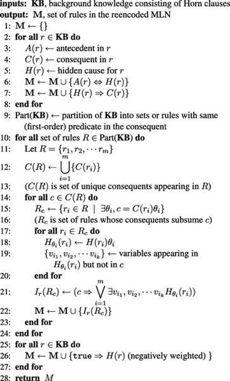
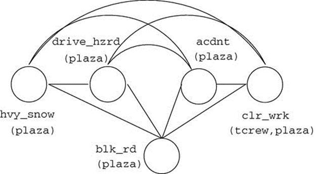
FIGURE 3.3 Ground network constructed by the PC model for the roadblock example.

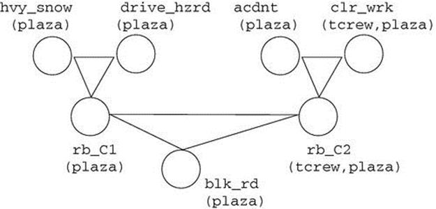
FIGURE 3.4 Ground network constructed by the HC model for the roadblock example.

Algorithm 3.2 presents the pseudocode for constructing the reencoded MLN using the HC approach for a given Horn-clause KB. In lines 2 to 8, hidden causes are created for each possible explanation for each consequent (line 5). A biconditional is introduced between the hidden causes and the corresponding antecedents (line 6), which is modeled as a soft clause in the MLN. Each HC is also linked to the corresponding consequent via a hard clause (line 7).

The next part (lines 9 to 24) combines the hidden causes for each of the consequents into a single reverse implication. The rules are partitioned according to the first-order predicate appearing in the consequent (line 9). For each partition (line 10), each possible instantiation of the consequent predicate appearing in the underlying rule is considered (lines 11 to 13). For instance, given the rules and another, , we need to consider each instantiation of and separately. For each such instantiation (line 14), we consider the rules that could result in the consequent being true (line 15).

Technically, these are rules with consequents that subsume (i.e., there exists a substitution such that , where is the consequent of rule ). These rules result in when bound by the substitution . For each such rule (line 17), substitution is applied to the corresponding hidden cause (line 18). Then, the set of free variables in the HC (i.e., the variables not appearing in ) is extracted (line 19). These variables are existentially quantified in the reverse implication (next step). We then introduce a reverse implication to indicate that implies at least one of the consequents among those that subsume (line 21). This reverse implication is made a hard clause and added to the MLN (line 22). Finally, a low prior is introduced for each hidden cause (lines 25 to 27).

3.4.3 Abductive Model Construction

Abductive reasoning using MLNs consists of the following three steps:

1. Generate the reencoded MLN.

2. Construct the ground Markov network (model construction).

3. Perform learning/inference over the resulting ground network.

The standard MLN model-construction process uses the set of all possible ground atoms (the Herbrand base) and constructs the set of all possible ground clauses using these atoms.

Using logical rules to construct a graphical model is generally referred to as knowledge-based model construction, originally proposed by Wellman [66,4]. This idea was further used by Ngo and Haddawy [46] for answering queries from probabilistic knowledge bases. In abductive reasoning, we are looking for explanations for a given set of observations. In this task, the set of all possible ground atoms and ground clauses may not be needed to explain the observations. Considering the fully ground network leads to increased time and memory complexity for learning and inference. For instance, in the road-blocked example, if the observation of interest is , then we can ignore groundings when the location is not .

We propose an alternative model-construction procedure that uses logical abduction to determine the set of relevant ground atoms. The procedure first constructs the set of abductive proof trees for the observations and then uses only the ground atoms in these proofs instead of the full Herbrand base for constructing the ground network. The ground Markov network is then constructed by instantiating the formulae in the abductive MLN using this reduced set of ground atoms. We refer to the set of ground atoms (Markov network) thus constructed as the abductive ground atoms (Markov network).

First, given a set of Horn rules and a set of observations, the rules for the abductive MLN are constructed using the HC model. Next, the set of most-specific abductive proof trees for the observations are computed using the method of Stickel [65]. The abductive inference process to get the set of most-specific abductive proofs was described earlier in Algorithm 3.1. The atoms in these proofs form the set of abductive ground atoms. For each formula in the abductive MLN, the set of all ground formulae with atoms that appear in the abductive ground atoms are added to the ground Markov network. While handling existentials, only those disjuncts that belong to the set of abductive ground atoms are used. Learning and inference are then performed over the resulting network.

In general, the abductive model-construction procedure results in a ground network that is substantially different (and usually much simpler) from the one constructed using the full Herbrand base. It also differs from the network constructed by starting KBMC from the query/observations (see Domingos and Lowd [14]) because of the use of backward-chaining and unification during the abductive model construction. Consequently, the probabilistic inferences supported by this model can be different from those of the traditional MLN model. This also makes the abductive process different from other preprocessing approaches, such as Shavlik and Natarajan [61], or existing lifted inference techniques, such as Singla and Domingos [63], both of which produce a network that is probabilistically equivalent to the original.

By focusing on the relevant ground atoms, abductive model construction significantly improves the performance of abductive MLNs both in terms of time and memory efficiency and predictive accuracy. Further, lifted inference could still be applied by constructing a lifted network over the nodes/clauses present in the abductive network. For consistency with Singla and Mooney [64], we will refer to abductive MLNs (using the HC model followed by abductive model construction) as MLN-HCAM.

Detailed experiments demonstrating significantly improved plan-recognition performance (with respect to both accuracy and efficiency) for the HC model and abductive model construction are presented by Singla and Mooney [64]. Therefore, we only compare with the MLN-HCAM approach in the experiments that follow.

3.4.4 Plan Recognition Using Manually Encoded MLNs

As discussed in the introduction, traditional (nonabductive) MLNs can be used for plan recognition if an appropriate set of clauses are manually provided that directly infer higher-level plans from primitive actions (e.g., Sadilek and Kautz [58,57]). To compare to this approach, we developed an MLN approach that uses a manually engineered KB to perform deductive plan recognition.

The clauses for this manually encoded MLN were constructed as follows. For each top-level plan predicate, we identified any set of observations that uniquely identifies this plan. This implies that no other plan explains this set of observations. We then introduced a rule that infers this plan given these observations and we made it an HC in the MLN. If no such observations existed, we introduced a soft rule for each observation that could potentially indicate this plan. Hard mutual-exclusivity rules were included for plans when we knew only one of them could be true.

Alternatively, we gave a negative prior to all plan predicates as described in the MLN-HCAM model. Note that this approach does not include any predicates corresponding to subgoals that are never observed in the data. As a result, all variables in this model are fully observed during training, resulting in a less complex model for learning and inference. This way of encoding the domain knowledge avoids the automated machinery for introducing reverse implications and can potentially lead to a simpler knowledge base, which results in simpler ground networks. However, it requires a separate knowledge-engineering process that develops explicit plan-recognition rules for the domain, while the abductive approach only requires basic knowledge about plans and actions sufficient for planning. There are several ways in which such explicit plan-recognition KB can be manually engineered, and we have employed just one possible approach. Exploring alternative approaches is a direction for future work. Subsequently, we refer to this manually encoded traditional MLN model as “MLN-manual.”

3.4.5 Probabilistic Modeling, Inference, and Learning

In MLN-HC and MLN-HCAM, we use the noisy-or model to combine multiple explanations. In all MLN models, we use the cutting-plane method of Riedel [56] for MPE inference and MC-SAT (see Poon and Domingos [51]) to compute marginal probabilities of plan instances. For learning weights of the clauses in MLN-HCAM, we use a version of gradient-based voted-perceptron algorithm of Singla and Domingos [62] modified for partially observed data as discussed in Chapter 20 (Section 3.3.1) of Koller and Friedman [40]. For the traditional MLN model, gradient-based voted-perceptron algorithm runs out of memory due to the size and complexity of the resulting ground networks. Therefore, we learned weights using the discriminative online learner proposed by Huynh and Mooney [24].¹ More details about various settings used in our experiments are described in the next section.

3.5 Experimental Evaluation

This section presents an extensive experimental evaluation of the performance of BALPs and MLNs on three plan-recognition datasets. Unfortunately, there have been very few rigorous empirical evaluations of plan-recognition systems, and there are no widely used benchmarks. Our experiments employ three extant datasets and compare them to the state-of-the-art results in order to demonstrate the advantages of SRL methods. In addition to presenting concrete results for BALPs and MLNs, we consider their relationship to other probabilistic logics, discussing the relative strengths and weaknesses of different SRL models for plan recognition.

3.5.1 Datasets

3.5.1.1 Story Understanding

We first used a small dataset previously employed to evaluate abductive Story Understanding systems (see Ng and Mooney [45] and Charniak and Goldman [8]).² In this task, characters’ higher-level plans must be inferred from the actions described in a narrative text. A logical representation of the literal meaning of the text is given for each example. A sample story (in English) is: “Bill went to the liquor store. He pointed a gun at the owner.” The plans in this dataset include shopping, robbing, restaurant dining, traveling in a vehicle (e.g., bus, taxi, or plane), partying, and jogging. Most narratives involve more than a single plan. This small dataset consists of 25 development examples and 25 test examples each containing an average of 12.6 literals. We used the planning background knowledge initially constructed for the ACCEL system of Ng and Mooney [45], which contains a total of 126 Horn rules.

3.5.1.2 Monroe

We also used the Monroe dataset, an artificially generated plan-recognition dataset in the emergency-response domain by Blaylock and Allen [2]. This domain includes 10 top-level plans (e.g., setting up a temporary shelter, clearing a car wreck, and providing medical attention to victims). The task is to infer a single instantiated top-level plan based on a set of observed actions automatically generated by a hierarchical transition network (HTN) planner. We used the logical plan KB for this domain constructed by Raghavan and Mooney [54] which consists of 153 Horn clauses. We used 1000 artificially generated examples in our experiments. Each example instantiates one of the 10 top-level plans and contains an average of 10.19 ground literals describing a sample execution of this plan.

3.5.1.3 Linux

The Linux data is another plan-recognition dataset created by Blaylock and Allen [3]. Human users were asked to perform various tasks in Linux and their commands were recorded. The task is to predict the correct top-level plan from the sequence of executed commands. For example, one of the tasks involves finding all files with a given extension. The dataset contains 19 top-level plan schemas and 457 examples, with an average of 6.1 command literals per example. Here again, we used the plan KB constructed by Raghavan and Mooney [54] which consists of 50 Horn clauses.

Each of these datasets evaluates a distinct aspect of plan-recognition systems. Since the Monroe domain is quite large with numerous subgoals and entities, it tests the ability of a plan-recognition system to scale to large domains. On the other hand, the Linux dataset is not that large, but since the data comes from real human users, it is quite noisy. There are several sources of noise including cases in which users claim that they have successfully executed a top-level plan when actually they have not [2]. Therefore, this dataset tests the robustness of a plan-recognition system with noisy input. Monroe and Linux involve predicting a single top-level plan; however, in the Story Understanding domain, most examples have multiple top-level plans. Therefore, this dataset tests the ability of a plan-recognition system to identify multiple top-level plans.

3.5.2 Comparison of BALPs, MLNs, and Existing Approaches

This section presents experimental results comparing the performance of BALPs and MLNs to those of existing plan-recognition approaches (e.g., ACCEL [45]) and the system developed by Blaylock and Allen [2]. ACCEL is a purely logical abductive reasoning system that uses a variable evaluation metric to guide its search for the best explanation. It can use two different evaluation metrics: simplicity, which selects the explanation with the fewest assumptions, and coherence, which selects the explanation that maximally connects the input observations [10]. This second metric is specifically geared toward text interpretation by measuring explanatory coherence described by Ng and Mooney [44]. Currently, this bias has not been incorporated into either BALPs or any of the MLN approaches. Blaylock and Allen’s system is a purely probabilistic system that learns statistical -gram models to separately predict plan schemas (i.e., predicates) and their arguments.

Section 3.4 describes several variants of MLNs for plan recognition. All MLN models were implemented using Alchemy [39], an open-source software package for learning and inference in Markov logic. We used the logical abduction component developed for BALPs (see Algorithm 3.1) for abductive model construction in MLNs. Since this abductive Markov logic formulation (MLN-HCAM) performs better than simple reencodings of the traditional MLN, we restrict our comparative experiments to this approach. For more details on the experimental results comparing the different MLN enhancements, we refer the reader to Singla and Mooney [64]. For the Monroe and Linux datasets, we also compare with the traditional (nonabductive) MLN approach described in Section 3.4.4, referred to as “MLN-manual.”

For BALPs, we learned the noisy-or parameters using the EM algorithm described in Section 3.3.2 whenever possible. Similarly, for both MLN-HCAM and MLN, we learned the parameters using the algorithms described in Section 3.4.5. For datasets that had multiple top plans as the explanation, we computed the MPE. For datasets that had a single correct top-level plan, we computed the marginal probability of plan instances and picked the one with the highest marginal probability. For both MLNs and BALPs, we used exact inference whenever feasible. However, when exact inference was intractable, we used approximate sampling to perform probabilistic inference—SampleSearch detailed by Gogate and Dechte [17] for BALPs and MC-SAT by Poon and Domingos [51] for MLNs. Both these techniques are approximate sampling algorithms designed for graphical models with deterministic constraints. Whenever we deviate from this standard methodology, we provide the specific details.

3.5.2.1 Story Understanding

This section provides information on the methodology and results for experiments on the Story Understanding dataset.

Parameter learning

For BALPs, we were unable to learn effective parameters from the mere 25 development examples. As a result, we set parameters manually in an attempt to maximize performance on the development set. A uniform value of 0.9 for all noisy-or parameters seemed to work well for this domain. The intuition behind our choice of noisy-or parameters is as follows: If a parent node is true, then with a probability of 0.9, the child node will be true. In other words, if a cause is true, then the effect is true with the probability of 0.9.

Using the deterministic logical-and model to combine evidence from conjuncts in the body of a clause did not yield high-quality results. Using noisy-and significantly improved the results; so we used noisy-ands with uniform parameters of 0.9. Here again, the intuition is that if a parent node is false or turned off, then the child node would also be false or turned off with a probability of 0.9. To disambiguate between conflicting plans, we set different priors for high-level plans to maximize performance on the development data. For MLN-HCAM, we were able to learn more effective weights from the examples in the development set using the learning algorithm described in Section 3.4.5.

Probabilistic inference

Since multiple plans are possible in this domain, we computed the MPE to infer the best set of plans. Since the resulting graphical models for this domain were not exceptionally large, we were able to apply exact, rather than approximate, inference algorithms. For BALPs, we used the k-MPE algorithm described by Nilsson [47] as implemented in ELVIRA [15]. For MLN-HCAM, we used the cutting-plane method, and its associated code, developed by Riedel [56].

Evaluation metrics

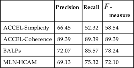
We compared BALPs and MLN-HCAM with ACCEL-Simplicity and ACCEL-Coherence. We compared the inferred plans with the ground truth to compute precision (percentage of the inferred plans that are correct), recall (percentage of the correct plans that were properly inferred), and F-measure (harmonic mean of precision and recall). Partial credit was given for predicting the correct plan predicate with some incorrect arguments. A point was rewarded for inferring the correct plan predicate, then, given the correct predicate, an additional point was rewarded for each correct argument. For example, if the correct plan was and the inferred plan was , the score is .

Results

Table 3.1 shows the results for Story Understanding. Both BALPs and MLN-HCAM perform better than ACCEL-Simplicity, demonstrating the advantage of SRL models over standard logical abduction. BALPs perform better than MLN-HCAM, demonstrating an advantage of a directed model for this task. However, ACCEL-Coherence still gives the best results. Since the coherence metric incorporates extra criteria specific to Story Understanding, this bias would need to be included in the probabilistic models to make them more competitive. Incorporating this bias into SRL models is difficult since it uses the graphical structure of the abductive proof to evaluate an explanation, which is not straightforward to include in a probabilistic model. It should be noted that the coherence metric is specific to narrative interpretation, since it assumes the observations are connected in a coherent “story,” and this assumption is not generally applicable to other plan-recognition problems.

Table 3.1

Results for the Story Understanding Dataset

3.5.2.2 Monroe and Linux

This section provides information on the methodology and results for experiments on the Monroe and Linux datasets.

Parameter learning

For BALPs, we learned the noisy-or parameters automatically from data using the EM algorithm described in Section 3.3.2. We initially set all noisy-or parameters to 0.9, which gave reasonable performance in both domains. We picked a default value of 0.9 based on the intuition that if a parent node is true, then the child node is true with a probability 0.9. We then ran EM with two starting points: random weights and manual weights (0.9). We found that EM initialized with manual weights generally performed the best for both domains; thus, we used this approach for our comparisons. Even though EM is sensitive to its starting point, it outperformed other approaches even when initialized with random weights. For Monroe and Linux, initial experiments found no advantage to usingnoisy-and instead of logical-and in these domains, so we did not experiment with learning noisy-and parameters.

For MLN-HCAM, we learned the weights automatically from data using the methods described in Section 3.4.5. For MLN-manual, the online weight learner did not provide any improvement over default manually encoded weights (a weight of 1 for all the soft clauses and a weight of −0.5 on unit clauses for all plan predicates to specify a small prior for all plans). Therefore, we report results obtained using these manually encoded weights.

For Monroe, of the 1000 examples in our dataset we used the first 300 for training, the next 200 for validation, and the remaining 500 for tests. Blaylock and Allen learned their parameters on 4500 artificially generated examples. However, we found that using a large number of examples resulted in much longer training times and that 300 examples were sufficient to learn effective parameters for both BALPs and MLN-HCAM. For BALPs, we ran EM on the training set until we saw no further improvement in the performance on the validation set. For MLN-HCAM, the parameter learner was limited to training on at most 100 examples because learning on larger amounts of data ran out of memory. Therefore, we trained MLN-HCAM on three disjoint subsets of the training data and picked the best model using the validation set.

For Linux, we performed 10-fold cross-validation. For BALPs, we ran EM until convergence on the training set for each fold. For MLN-HCAM, within each training fold, we learned the parameters on disjoint subsets of data, each consisting of around 110 examples. As mentioned before for Monroe, the parameter learner did not scale to larger datasets. We then used the rest of the examples in each training fold for validation, picking the model that performed best on the validation set.

As discussed in Section 3.4.4, in the traditional MLN model, there are two ways to encode the bias that only a single plan is needed to explain a given action. The first approach is to include explicit hard mutual-exclusivity constraints between competing plans; the second approach involves setting a low prior on all plan predicates. While the former performed better on Monroe, the latter gave better results on Linux. We report the results of the best approach for each domain.

As noted, we had to adopt a slightly different training methodology for BALPs and MLN-HCAM because of computational limitations of MLN weight learning on large datasets. However, we used the exact same test sets for both systems on all datasets. Developing more scalable online methods for training MLNs on partially observable data is an important direction for future work.

Probabilistic inference

Both Monroe and Linux involve inferring a single top-level plan. Therefore, we computed the marginal probability of each plan instantiation and picked the most probable one. For BALPs, since exact inference was tractable on Linux, we used the exact inference algorithm implemented in Netica,³ a commercial Bayes net software package. For Monroe, the complexity of the ground network made exact inference intractable and we used SampleSearch [17], an approximate sampling algorithm for graphical models with deterministic constraints. For both MLN approaches, we used MC-SAT [51] as implemented in the Alchemy system on both Monroe and Linux.

Evaluation metric

We compared the performance of BALPs, MLN-HCAM, and MLN with Blaylock and Allen’s system using the convergence score as defined by them [2]. The convergence score measures the fraction of examples for which the correct plan predicate is inferred (ignoring the arguments) when given all of the observations. Use of the convergence score allowed for the fairest comparison to the original results on these datasets published by Blaylock and Allen.⁴

Results

Table 3.2 shows convergence scores for the Monroe and Linux datasets. Both BALPs and MLN-HCAM recognize plans in these domains more accurately than Blaylock and Allen’s system. The performance of BALPs and MLN-HCAM are fairly comparable on Monroe; however, BALPs are significantly more accurate on Linux. The traditional MLN performs the worst and does particularly poorly on Linux. This demonstrates the value of the abductive approach as implemented in MLN-HCAM.

Table 3.2

Convergence Scores for Monroe and Linux Datasets

Partial observability results

The convergence score has the following limitations as a metric for evaluating the performance of plan recognition:

• It only accounts for predicting the correct plan predicate, ignoring the arguments. In most domains, it is important for a plan-recognition system to accurately predict arguments as well. For example, in the Linux domain, if the user is trying to move test1.txt totest-dir, it is not sufficient to just predict the move command; it is also important to predict the file (test.txt) and the destination directory (test-dir).

• It only evaluates plan prediction after the system has observed all of the executed actions. However, in most cases, we would like to be able to predict plans after observing as few actions as possible.

To evaluate the ability of BALPs and MLNs to infer plan arguments and to predict plans after observing only a partial execution, we conducted an additional set of experiments. Specifically, we performed plan recognition after observing the first 25%, 50%, 75%, and 100% of the executed actions. To measure performance, we compared the complete inferred plan (with arguments) to the gold standard to compute an overall accuracy score. As for Story Understanding, partial credit was given for predicting the correct plan predicate with only a subset of its correct arguments.

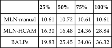
Table 3.3 shows the results for partial observability for the Monroe data. BALPs perform slightly better than MLN-HCAM on higher levels of observability, whereas MLN-HCAM tends to outperform BALPs on lower levels of observability. MLN-manual performs worst at higher levels of observability, but at 25% observability, it outperforms BALPs. Table 3.4 shows the results for partial observability on the Linux data. Here, BALPs clearly outperform MLN-HCAM and traditional MLNs at all the levels of observability. The traditional MLN performs significantly worse than the other two models, especially at higher levels of observability. For Story Understanding, since the set of observed actions is already incomplete, we did not perform additional experiments for partial observability.

Table 3.3

Accuracy on Monroe Data for Varying Levels of Observability

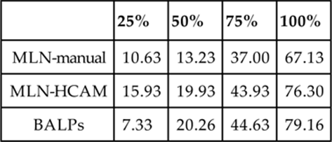
Table 3.4

Accuracy on Linux Data for Varying Levels of Observability

3.5.2.3 Discussion

We believe several aspects of SRL approaches led to their superior performance over existing approaches such as ACCEL and Blaylock and Allen’s system. The ability of BALPs and MLN-HCAM to perform probabilistic reasoning most likely resulted in their improved performance over ACCEL-Simplicity, a standard logical abduction method. When Blaylock and Allen [2] perform instantiated plan recognition, it is done in a pipeline of two separate steps. The first step predicts the plan schema and the second step predicts the arguments given the schema. Unlike their approach, BALPs and MLN-HCAM are able to jointly predict both the plan schema and its arguments simultaneously.

We believe that this ability of SRL models to perform joint prediction of plans and their arguments is at least partially responsible for their superior performance. In addition, both BALPs and MLN-HCAM use prior planning knowledge encoded in the logical clauses given to the system, while Blaylock and Allen’s system has no access to such planning knowledge. We believe that the ability of SRL models to incorporate such prior domain knowledge also contributes to their superior performance.

MLN-manual, although a joint model, cannot take advantage of all the domain knowledge in the planning KB available to BALPs and MLN-HCAM. Also, it does not have the advantages offered by the abductive model-construction process used in MLN-HCAM. This also makes it difficult to adequately learn the parameters for this model. We believe these factors led to its overall inferior performance compared to the other models.

For both the Monroe and Linux domains, the relative gap in the performance of MLN-manual model decreases with decreasing observability. This is particularly evident in Linux, where the performance stays almost constant with decreasing observability. We believe this is due to the model’s ability to capitalize on even a small amount of information that deterministically predicts the top-level plan. Furthermore, at lower levels of observability, the ground networks are smaller and, therefore, approximate inference is more likely to be accurate.

Singla and Mooney [64] report that MLN-PC and MLN-HC models did not scale well enough to make them tractable for the Monroe and Linux domains. When compared to these models, MLN-manual has a substantial advantage; however, it still does not perform nearly as well as the MLN-HCAM model. This reemphasizes the importance of using a model that is constructed by focusing on both the query and the available evidence. Furthermore, the MLN-manual approach requires costly human labor to engineer the knowledge base. This is in contrast to the abductive MLN models that allow the same KB to be used for both planning and plan recognition.

Comparing BALPs and MLN-HCAM, BALPs generally performed better. We believe this difference is in part due to the advantages that directed graphical models have for abductive reasoning, as originally discussed by Pearl [48]. Note that MLN-HCAM already incorporates several ideas that originated with BALPs. By using hidden causes and noisy-or to combine evidence from multiple rules, and by using logical abduction to obtain a focused set of literals for the ground network, we improved the performance of MLNs by making them produce a graphical model that is more similar to the one produced by BALPs.

Although, in principle, any directed model can be reexpressed as an undirected model, the learning of parameters in the corresponding undirected model can be significantly more complex since there is no closed-form solution for the maximum-likelihood set of parameters, unlike in the case of directed models⁵[40]. Inaccurate learning of parameters can lead to potential loss of accuracy during final classification. Undirected models do have the advantage of representing cyclic dependencies (e.g., transitivity), which directed models cannot represent explicitly because of the acyclicity constraint. But we did not find it particularly useful for plan recognition since domain knowledge is expressed using rules that have inherent directional (causal) semantics. In addition, it is very difficult to develop a general MLN method that constructs a Markov net that is formally equivalent to the Bayes net constructed by a BALP given the same initial planning knowledge base.

In general, it took much more engineering time and effort to get MLNs to perform well on plan recognition compared to BLPs. Extending BLPs with logical abduction was straightforward. The main problem we encountered while adapting BLPs to work well on our plan-recognition benchmarks was finding an effective approximate inference algorithm that scaled well to the larger Monroe and Linux datasets. Once we switched to SampleSearch, which is designed to work well with the mix of soft and hard constraints present in networks, BALPs produced good results. However, getting competitive results with MLNs and scaling them to work with our larger datasets was significantly more difficult.

First, we needed to develop a method for properly introducing reverse clauses to allow MLNs to perform logical abduction. Next, we had to develop a method for introducing hidden causes to prevent the creation of networks with large cliques that made inference intractable. Finally, we had to develop an abductive model-construction process that used the ground literals constructed for BALPs to constrain the size and scope of the ground Markov net. Even after all these modifications, the weight learning algorithm did not scale to larger training sets, and the overall results are still not competitive with BALPs.

Some of the differences in the performance of BALPs and MLN-HCAM may also stem from the differences in the probabilistic inference and parameter learning algorithms employed. For instance, on the Linux dataset, we could run exact inference for BALPs; however, we had to resort to MC-SAT, an approximate sampling algorithm, for MLN-HCAM. On Monroe, even though we used approximate sampling algorithms for both BALPs and MLN-HCAM, it is unclear whether the performance of SampleSearch and MC-SAT are comparable. Furthermore, since probabilistic inference is used extensively during parameter learning, performance of the inference techniques could impact the quality of the learned weights/parameters.

In our preliminary work, we converted the noisy-or parameters learned using the EM algorithm for BALPs into weights in MLN-HCAM. When we performed plan recognition using these weights, we found that the performance of MLN-HCAM improved, demonstrating a lack of quality in the learned MLN weights. This could be due either to poor performance of probabilistic inference or to poor performance of the weight learner itself. Additional experiments that control for changes in the inference and learning algorithms are needed to further understand the effects of these differences.

3.5.3 Comparison of BALPs and MLNs to Other SRL Models

BLPs, BALPs, and MLNs are all languages for flexibly and compactly representing large, complex probabilistic graphical models. An alternative approach to SRL is to add a stochastic element to the deductive process of a logic program. ProbLog, described by Kimmig et al. [35], is the most recent and well developed of these approaches. ProbLog can be seen as extending and subsuming several previous models, such as Poole’s Probabilistic Horn Abduction (PHA) [50] and PRISM described by Sato [60]. Finally, there is publicly available implementation of ProbLog⁶ that exploits the latest inference techniques based on binary decision diagrams (BDDs) to provide scalability and efficiency.

Therefore, we attempted to also compare the performance of our models to ProbLog. It was relatively straightforward to develop a ProbLog program for plan recognition by appropriately formulating the planning KB used for both BLPs and abductive MLNs. However, our preliminary explorations with ProbLog revealed a serious limitation that prevented us from actually performing an experimental comparison on our plan-recognition datasets.

In a number of the planning axioms in our KBs, existentially quantified variables occur in the body of a clause that do not occur in the head. Representing these clauses in ProbLog requires binding such variables to all possible type-consistent constants in the domain. However, this results in the ProbLog inference engine attempting to construct an intractable number of explanations (i.e., proofs) due to the combinatorial number of possible combinations of the introduced constants. Therefore, it was intractable to run ProbLog on our datasets, preventing an empirical comparison. BALPs and MLN-HCAM use a greedy abductive proof-construction method described in Section 3.3.1 to prevent this combinatorial explosion. Therefore, we believe ProbLog would need a new approximate inference algorithm for this situation in order to be practically useful for plan recognition.

Abductive Stochastic Logic Programs (ASLPs), described by Chen et al. [12] are another SRL model that uses stochastic deduction and supports logical abduction and therefore could potentially be applied to plan recognition. However, we are unaware of a publicly available implementation of ASLPs that could be easily used for experimental comparisons.

3.6 Future Work

The research presented in this chapter could be extended in various ways. First, it would be good to evaluate the proposed plan-recognition systems on additional domains and applications. Unfortunately, there are very few publicly available datasets for plan recognition. Second, the existing SRL methods could be improved and extended in several productive directions.

Methods for lifted inference proposed by Singla and Domingos [63] could improve efficiency by allowing probabilistic inference to be performed without having to explicitly construct complete ground networks. In particular, the latest Probabilistic Theorem Proving (PTP) methods for lifted inference in MLNs, described by Gogate and Domingos [18], could be tried to improve the efficiency and accuracy of the MLN models.

Improved online weight learning algorithms could be developed to more efficiently train on large datasets and increase the accuracy of the learned models. In particular, discriminative rather than generative (i.e., EM) parameter learning for BALPs should be explored. Although discriminative learning is more difficult for directed graphical models than for undirected ones, Carvalho et al. [7] have made recent progress on this problem. Current discriminative online weight learners for MLNs, described by Huynh and Mooney [24], assume completely observable training data. These methods are not applicable to abductive MLNs, which contain unobserved subgoals and noisy-or nodes. Therefore, effective online methods for partially observed training data need to be developed.

With respect to the traditional MLN approach, better methods for manually engineering effective rules for deductive plan recognition could be developed. Alternatively, MLN structure learning (e.g., Kok and Domingos [36,38] and Huynh and Mooney [25]) could be used to automatically induce such rules from supervised training data. In addition, a similar approach could be developed for applying traditional (deductive) BLPs to plan recognition.

The current experimental comparisons should be extended to additional SRL models. As mentioned in Section 3.5.3, an improved approximate inference method is needed to make ProbLog tractable for our plan-recognition problems. Comparisons to other SRL models, such as Poole’s Horn Abduction [50], PRISM [60], and Abductive Stochastic Logic Programs [12], are also indicated.

3.7 Conclusion

This chapter has introduced two new SRL approaches to plan recognition, one based on Bayesian Logic Programs and another on Markov Logic Networks. Both approaches combine the advantages of prior logical and probabilistic methods. We presented novel techniques for extending both MLNs and BLPs with logical abduction in order to allow for plan recognition given logical definitions of actions and plans as the only prior knowledge. Experimental evaluations on three benchmark datasets have shown that our approaches generally outperform other state-of-the-art plan-recognition methods. We believe their superior performance is due to the combination of logical abduction, joint probabilistic inference, and incorporation of planning domain knowledge. The results also indicate that the approach based on BLPs is generally more effective than the one based on MLNs.

References

1. Albrecht DW, Zukerman I, Nicholson AE. Bayesian models for keyhole plan recognition in an adventure game. User Model User-Adap Intract. 1998;8(1–2):5-47.

2. Blaylock N, Allen J. Recognizing instantiated goals using statistical methods. In: Kaminka G, editor. Workshop on modeling others from observations; 2005. p. 79–86.

3. Blaylock N, Allen JF. Statistical goal parameter recognition. Proceedings of the 14th International Conference on Automated Planning and Scheduling. 2004:297-305.

4. Breese JS, Goldman RP, Wellman MP. Introduction to the special section on knowledge-based construction of probabilistic and decision models. IEEE Trans Syst Man Cybern. 1994;24(11):1577-1579.

5. Bui HH. A general model for online probabilistic plan recognition. Proceedings of the 18th International Joint Conference on Artificial Intelligence. 2003:1309-1315.

6. Bui HH, Venkatesh S, West G. Policy recognition in abstract hidden Markov model. J Artif Intell Res. 2002;17:451-499.

7. Carvalho AM, Roos T, Oliveira AL, Myllymäki P. Discriminative learning of Bayesian networks via factorized conditional log-likelihood. J Mach Learn Res. 2011;12:2181-2210.

8. Charniak E, Goldman R. A probabilistic model of plan recognition. Proceedings of the Ninth National Conference on Artificial Intelligence. 1991:60-165.

9. Charniak E, Goldman RP. A semantics for probabilistic quantifier-free first-order languages, with particular application to story understanding. Proceedings of the 11th International Joint Conference on Artificial Intelligence. 1989:1074-1079.

10. Charniak E, Goldman RP. Plan recognition in stories and in life. Proceedings of the Fifth Annual Conference on Uncertainty in Artificial Intelligence. 1990:343-352.

11. Charniak E, McDermott D. Introduction to artificial intelligence. Addison-Wesley; 1985.

12. Chen J, Muggleton S, Santos J. Learning probabilistic logic models from probabilistic examples. Mach Learn. 2008;73(1):55-85.

13. Davis J, Ong I, Struyf J, Costa VS, Burnside E, Page D. Change of representation for statistical relational learning. Proceedings of the 20th International Joint Conference on Artificial Intelligence. 2007:2719-2726.

14. Domingos P, Lowd D. Markov logic: an interface layer for artificial intelligence. Morgan & Claypool; 2009.

15. Elvira-Consortium. ELVIRA: an environment for probabilistic graphical models. Proceedings of the Workshop on Probabilistic Graphical Models. 2002:222-2 30.

16. Getoor L, Taskar B, eds. Introduction to statistical relational learning. MIT Press; 2007.

17. Gogate V, Dechter R. Samplesearch: importance sampling in presence of determinism. Artif Intell. 2011;175:694-729.

18. Gogate V, Domingos P. Probabilistic theorem proving. Proceedings of the 27th Annual Conference on Uncertainty in Artificial Intelligence. 2011:256-265.

19. Goldman RP, Geib CW, Miller CA. A new model for plan recognition. Proceedings of the 15th Conference on Uncertainty in Artificial Intelligence. 1999:245-254.

20. Hobbs JR, Stickel ME, Martin P, Edwards D. Interpretation as abduction. Proceedings of the 26th Annual Meeting of the Association for Computational Linguistics. 1988:95-103.

21. Hong J. Goal recognition through goal graph analysis. J Artif Intell Res. 2001;15:1-30.

22. Horvitz E, Paek T. A computational architecture for conversation. Proceedings of the Seventh International Conference on User Modeling. 1999:201-210.

23. Huber MJ, Durfee EH, Wellman MP. The automated mapping of plans for plan recognition. Proceedings of the Tenth Conference on Uncertainty in Artificial Intelligence. 1994:344-351.

24. Huynh TN, Mooney RJ. Online max-margin weight learning for Markov logic networks. Proceedings of the 11th SIAM International Conference on Data Mining. 2011:642-651.

25. Huynh TN, Mooney RJ. Online structure learning for Markov Logic Networks. Proceedings of the European Conference on Machine Learning and Principles and Practice of Knowledge Discovery in Databases. 2011:81-96.

26. Inoue N, Ovchinnikova E, Inui K, Hobbs J. Weighted abduction for discourse processing based on integer linear programming. In: Sukthankar G, Goldman RP, Geib C, Pynadath DV, Bui HH, eds. Plan, activity, and intent recognition: theory and practice. Waltham, MA: Morgan Kaufmann Publishers; 2014:33-356.

27. Kakas AC, Kowalski RA, Toni F. Abductive logic programming. J Logic Comput. 1993;2(6):719-770.

28. Kaminka GA, Pynadath DV, Tambe M. Monitoring teams by overhearing: a mulit-agent plan-recognition approach. J Artif Intell Res. 2002;17:83-135.

29. Kate RJ, Mooney RJ. Probabilistic abduction using Markov logic networks. In: Proceedings of the Workshop on Plan, Activity, and Intent Recognition; 2009.

30. Kautz HA. A formal theory of plan recognition. Ph.D. Thesis. Department of Computer Science. University of Rochester. Technical Report 215; 1987.

31. Kautz HA, Allen JF. Generalized plan recognition. Proceedings of the Fifth National Conference on Artificial Intelligence. 1986:32-37.

32. Kersting K, De Raedt L. Towards combining inductive logic programming with Bayesian networks. Proceedings of the 11th International Conference on Inductive Logic Programming. 2001:118-131.

33. Kersting K, De Raedt L. Bayesian logic programming: Theory and tool. In: Getoor L, Taskar B, eds. Introduction to statistical relational learning. MIT Press; 2007.

34. Kersting K, de Raedt L. Basic principles of learning Bayesian logic programs. In: De Raedt L, Frasconi P, Kersting K, Muggleton S, eds. Probabilistic inductive logic programming. Springer; 2008:189-221.

35. Kimmig A, Santos Costa V, Rocha R, Demoen B, De Raedt L. On the efficient execution of ProbLog programs. Proceedings of the 24th International Conference on Logic Programming. 2008:175-189.

36. Kok S, Domingos P. Learning the structure of Markov logic networks. Proceedings of 22nd International Conference on Machine Learning. 2005:441-448.

37. Kok S, Domingos P. Statistical predicate invention. Proceedings of 24th International Conference on Machine Learning. 2007:433-440.

38. Kok S, Domingos P. Learning Markov logic networks using structural motifs. Proceedings of the 27th International Conference on Machine Learning. 2010:551-558.

39. Kok S, Sumner M, Richardson M, Singla P, Poon H, Lowd D, et al. The alchemy system for statistical relational AI. University of Washington. Technical Report. Department of Computer Science and Engineering; 2010.

40. Koller D, Friedman N. Probabilistic graphical models: principles and techniques. MIT Press; 2009.

41. Lesh N, Etzioni O. A sound and fast goal recognizer. Proceedings of the 14th International Joint Conference on Artificial Intelligence. 1995:1704-1710.

42. Levesque HJ. A knowledge-level account of abduction. Proceedings of the 11th International Joint Conference on Artificial Intelligence. 1989:1061-1067.

43. Natarajan S, Khot T, Kersting K, Tadepalli P, Shavlik J. Exploiting causal independence in Markov logic networks: Combining undirected and directed models. Proceedings of the European Conference on Machine Learning and Principles and Practice of Knowledge Discovery in Databases. 2010:434-450.

44. Ng HT, Mooney RJ. The role of coherence in abductive explanation. Proceedings of the Eighth National Conference on Artificial Intelligence. 1990:337-442.

45. Ng HT, Mooney RJ. Abductive plan recognition and diagnosis: A comprehensive empirical evaluation. Proceedings of the Third International Conference on Principles of Knowledge Representation and Reasoning. 1992:499-508.

46. Ngo L, Haddawy P. Answering queries from context-sensitive probabilistic knowledge bases. Theor Comput Sci. 1997;171:147-177.

47. Nilsson D. An efficient algorithm for finding the M most probable configurations in probabilistic expert systems. Stat Comput. 1998;8:159-173.

48. Pearl J. Probabilistic reasoning in intelligent systems: networks of plausible inference. Morgan Kaufmann; 1988.

49. Peng Y, Reggia JA. Abductive inference models for diagnostic problem-solving. Springer-Verlag; 1990.

50. Poole D. Probabilistic Horn abduction and Bayesian networks. Artif Intell. 1993;64:81-129.

51. Poon H, Domingos P. Sound and efficient inference with probabilistic and deterministic dependencies. Proceedings of the 21st National Conference on Artificial Intelligence. 2006:458-463.

52. Pople HE. On the mechanization of abductive logic. Proceedings of the Third International Joint Conference on Artificial Intelligence. 1973:147-152.

53. Pynadath DV, Wellman MP. Probabilistic state-dependent grammars for plan recognition. Proceedings of the Conference on Uncertainty in Artificial Intelligence. 2000:507-514.

54. Raghavan S, Mooney RJ. Abductive plan recognition by extending Bayesian logic programs. Proceedings of the European Conference on Machine Learning and Principles and Practice of Knowledge Discovery in Databases. 2011:629-644.

55. Richardson M, Domingos P. Markov logic networks. Mach Learn. 2006;62:107-136.

56. Riedel S. Improving the accuracy and efficiency of MAP inference for Markov logic. Proceedings of 24th Conference on Uncertainty in Artificial Intelligence. 2008:468-475.

57. Sadilek A, Kautz H. Modeling and reasoning about success, failure, intent of multi-agent activities. Proceedings of the UbiComp Workshop on Mobile Context Awareness. 2010.

58. Sadilek A, Kautz H. Recognizing multi-agent activities from GPS data. Proceedings of the 25th AAAI Conference on Artificial Intelligence. 2010:1134-1139.

59. Saria S, Mahadevan S. Probabilistic plan recognition in multiagent systems. Proceedings of the International Conference on Automated Planning and Scheduling. 2004:287-296.

60. Sato T. A statistical learning method for logic programs with distribution semantics. Proceedings of the 12th International Conference on Logic Programming. 1995:715-729.

61. Shavlik J, Natarajan S. Speeding up inference in Markov logic networks by preprocessing to reduce the size of the resulting grounded network. Proceedings of the 21st International Joint Conference on Artificial Intelligence. 2009:1951-1956.

62. Singla P, Domingos P. Discriminative training of Markov logic networks. Proceedings of the 20th National Conference on Artificial Intelligence. 2005:868-873.

63. Singla P, Domingos P. Lifted first-order belief propagation. Proceedings of the 23rd AAAI Conference on Artificial Intelligence. 2008:1094-1099.

64. Singla P, Mooney R. Abductive Markov logic for plan recognition. Proceedings of the 25th National Conference on Artificial Intelligence. 2011:1069-1075.

65. Stickel ME. A probLog-like inference system for computing minimum-cost abductive explanations in natural-language interpretation. Technical Note 451. SRI International; 1988.

66. Wellman MP, Breese JS, Goldman RP. From knowledge bases to decision models. Knowl Eng Rev. 1992;7(01):35-53.